11
Aircraft Drag
11.1 Overview
After the completion of the concept definition that concluded in Chapter 10, the next phase is to end the Phase I stage of the new aircraft project with concept finalisation through the formal method of aircraft sizing and engine matching exercise in Chapter 14 that will require aircraft performance analyses. This will require aircraft drag polar to be dealt with in this chapter and engine performance data to be dealt with in the next two chapters, Chapters 12 and 13.
An important task for aircraft performance engineers is to make the best possible estimation of all the different types of drag associated with aircraft aerodynamics. Commercial aircraft design is sensitive to the Direct Operating Cost (DOC), which is aircraft drag dependent. Just one count of drag (i.e. CD = 0.0001) could account for several million US dollars in operating cost over the lifespan of a small fleet of midsized aircraft. This becomes increasingly important with the trend in rising fuel costs. Accurate estimation of the different types of drag remains a central theme. (Equally important are other ways to reduce DOC; one of them is reducing manufacturing cost.)
For a century, a massive effort has been made to understand and estimate drag and the work is still continuing. Possibly some of the best work in English language on aircraft drag is compiled by National Advisory Committee for Aeronautics (NACA)/National Aeronautics and Space Administration (NASA), RAE (the Royal Aircraft Establishment), Advisory Group for Aerospace Research and Development (AGARD), Engineering Sciences Data Unit (ESDU), DATCOM (the short name for the USAF Data Compendium for Stability and Control) and others [1–11]. These publications indicate that the drag phenomena are still not fully understood [12] and that the way to estimate aircraft drag is by using semi‐empirical relations. Computational fluid dynamics (CFD) is gaining ground but it is still some way from supplanting the proven semi‐empirical relations. In the case of work on excrescence drag, efforts are lagging.
Two‐dimensional surface skin friction drag, elliptically loaded induced drag and wave drag can be accurately estimated – together, they comprise most of the total aircraft drag. The problem arises when estimating drag generated by the 3D effects of the aircraft body, interference effects and excrescence effects. In general, there is a tendency to underestimate aircraft drag. Accurate assessments of aircraft mass, drag and thrust are crucial in the aircraft performance estimation.
This chapter includes the following sections:
- Section 11.2: Introduction to Aircraft Drag
- Section 11.3: Parasite Drag
- Section 11.4: Aircraft Drag Breakdown Structure
- Section 11.5: Understanding Drag Polar
- Section 11.6: Theoretical Background of Aircraft Drag
- Section 11.7: Subsonic Aircraft Drag Estimation Methodology
- Section 11.8: Methodology to Estimate Minimum Parasite Drag (CDpmin)
- Section 11.9.1: Semi‐Empirical Relations to Estimate CDpmin
- Section 11.10: Excrescence Drag
- Section 11.11: Summary of Aircraft Parasite Drag (CDpmin)
- Section 11.12: Methodology to Estimate CDp
- Section 11.13: Methodology to Estimate Subsonic Wave Drag
- Section 11.14: Summary of Total Aircraft Drag
- Section 11.15: Low‐Speed Aircraft Drag at Takeoff and Landing
- Section 11.16: Drag of Propeller‐Driven Aircraft
- Section 11.17: Military Aircraft Drag
- Section 11.18: Empirical Methodology for Supersonic Drag Estimation
- Section 11.19: Bizjet Example – Civil Aircraft
- Section 11.20: Turboprop Example – Propeller‐Driven Aircraft
- Section 11.21: Military Aircraft Example
- Section 11.22: Classroom Example – Supersonic Military Aircraft
- Section 11.23: Drag Comparison
- Section 11.24: Some Concluding Remarks
Coursework content: Readers will carry out aircraft‐component drag estimation and obtain the total aircraft drag.
11.2 Introduction
The drag of an aircraft depends on its shape and speed, are design‐dependent, as well as on the properties of air, which are nature‐dependent. Drag is a complex phenomenon arising from several sources, such as the viscous effects that result in skin friction and pressure differences as well as the induced flow field of the lifting surfaces and compressibility effects (see Sections 4.9 and 4.11).
The aircraft drag estimate starts with the isolated aircraft components (e.g. wing and fuselage etc.). Each component of the aircraft generates drag, largely dictated by its shape. Total aircraft drag is obtained by summing the drag of all components plus their interference effects when the components are combined. The drag of two isolated bodies increases when they are brought together due to the interference of their flow fields.
The Reynolds Number (Re) has a deciding role in determining the associated skin friction coefficient, CF, over the affected surface and the type, extent, and steadiness of the boundary layer (which affects parasite drag) on it. Boundary‐layer separation increases drag and is undesirable; separation should be minimised.
A major difficulty arises in assessing drag of small items attached to an aircraft surface such as instruments (e.g. pitot and vanes), ducts (e.g. cooling), blisters and necessary gaps to accommodate moving surfaces. In addition, there are the unavoidable discrete surface roughness from mismatches (at assembly joints) and imperfections, perceived as defects that result from limitations in the manufacturing processes. Together, from both manufacturing and non‐manufacturing origins, they are collectively termed excrescence drag.
Currently, accurate total aircraft drag estimation by analytical or CFD methods is not possible. Schmidt of Dornier in the AGARD 256 [10] is categorical about the inability of CFD, analytical methods or even wind‐tunnel model‐testing to estimate drag. CFD is steadily improving and can predict wing‐wave drag (CDw) accurately but not the total aircraft drag – most of the errors are due to the smaller excrescence effects, interference effects and other parasitic effects. Industrial practices employ semi‐empirical relations (with CFD) validated against wind‐tunnel and flight tests and are generally proprietary information. Most of the industrial drag data are not available in the public domain. The methodology given in this chapter is a modified and somewhat simplified version of standard industrial practices [1, 3, 7, 8]. The method is validated by comparing its results with the known drag of existing operational aircraft.
The design criterion for today's commercial high‐subsonic jet‐transport aircraft is that the effects of separation and local shocks are minimised at the Long‐Range Cruise (LRC) at the MCR (when compressibility drag is almost equal to zero before the onset of wave drag) condition. At High‐Speed Cruise (HSC), a 20‐count drag increase is allowed, reaching Mcrit, due to local shocks (i.e. transonic flow) covering small areas of the aircraft. Modern streamlined shapes maintain low separation at Mcrit; therefore, such effects are small at HSC. The difference in the Mach number at HSC and LRC for subsonic aircraft is small – on the order of Mach 0.05–Mach 0.075. Aircraft drag characteristics are plotted as drag polar (CD vs CL).
Strictly speaking drag polar at several speed and altitudes will give better resolution of drag value however, estimation of the drag coefficient at LRC is sufficient because it has a higher Cf, which gives conservative values at HSC when ΔCDw is added. The LRC condition is by far the longest segment in the mission profile; the industry standard practice uses the LRC drag polar for all parts of the mission profile (e.g. climb and descent). The Re at the LRC provides a conservative estimate of drag at the climb and descent segments. At takeoff and landing, the undercarriage and high‐lift‐device drags must be added.
Supersonic aircraft operate over a wider speed range: the difference between Mcrit and maximum aircraft speed is on the order of Mach 1.0–Mach 1.2. Therefore, estimation of CDpmin is required at three speeds: (i) at a speed before the onset of wave drag at MCR, (ii) at Mcrit and (iii) at maximum speed (say, Mach 2.0).
It is difficult for the industry to absorb drag prediction errors of more than 5% (the goal is to ensure errors of less than 3%) for civil aircraft; overestimating, is better than underestimating. Practitioners are advised to be generous in allocating drag – it is easy to miss a few of the many sources of drag, as shown in the worked‐out examples in this chapter. Underestimated drag causes considerable design and management problems; failure to meet customer specifications is expensive for any industry. Subsonic aircraft drag prediction has advanced to the extent that most aeronautical establishments are confident in predicting drag with adequate accuracy. Military aircraft shapes are more complex; therefore, it is possible that predictions will be less accurate.
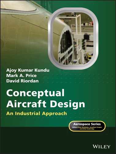
11.3 Parasite Drag Definition
The components of drag due to viscosity do not contribute to lift. For this reason, it is considered ‘parasitic’ in nature. For bookkeeping purposes, parasite drag is usually considered separately from other drag sources. The main components of parasite drag are as follows:
- drag due to skin friction
- drag due to the pressure difference between the front and the rear of an object
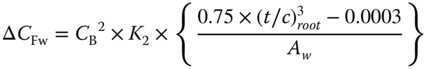
- drag due to the lift‐dependent viscous effect and therefore seen as parasitic (to some extent resulting from the non‐elliptical nature of lift distribution over the wing); this is a small but significant percentage, of total aircraft drag (at LRC, it is about 2–3%)
All of these components vary (to a small extent) with changes in aircraft incidence (i.e. as CL changes). The minimum parasite drag, CDpmin, occurs when shock waves and boundary‐layer separation are at a minimum, by design, around the LRC condition. Any change from the minimum condition (CDpmin) is expressed as ΔCDp. In summary:
Oswald's efficiency factor (see Section 4.9.3) is accounted for in the lift‐dependent parasite drag, ΔCDp. The nature of ΔCDp is specific to a particular aircraft. Numerically, it is small and difficult to estimate.
Parasite drag of a body depends on its form (i.e. shape) and is also known as form drag. The form drag of a wing profile is known as profile drag. These two terms are not used in this book. In the past, parasite drag in the Foot, Pound, Second (FPS) system was sometimes expressed as the drag force in pound force (lbf) at 100 ft s−1 speed, represented by D100. This practice was useful in its day as a good way to compare drag at a specified speed, but it is not used today.
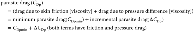
The current industrial practice using semi‐empirical methods to estimate CDpmin is a time‐consuming process. (If computerised, then faster estimation is possible, but the authors recommend relying more on the manual method at this stage.) Parasite drag constitutes half to two‐thirds of subsonic aircraft drag. Using the standard semi‐empirical methods, the parasite drag units of an aircraft and its components are generally expressed as the drag of the ‘equivalent flat plate area’ (or ‘flat plate drag’), placed normal to airflow as shown in Figure 11.1. These units are in square feet to correlate with literature in the public domain. This is not the same as air flowing parallel to the flat plate and encountering only the skin friction.
Figure 11.1 Flat plate equivalent of drag.
The inviscid idealisation of flow is incapable of producing parasite drag because of the lack of skin friction and the presence of full pressure recovery.
11.4 Aircraft Drag Breakdown (Subsonic)
There are many variations and definitions of the book‐keeping methods for components of aircraft drag; this book uses the typical US practice [2, 3]. The standard breakdown of aircraft drag is as follows (see Eq. 11.1):
Eq (4.22) gives CDi = CL2/eπAR
Therefore, the total aircraft drag coefficient is:
The advantage of keeping pure induced drag separate is obvious because it is dependent only on the lifting‐surface aspect ratio and is easy to compute. The total aircraft‐drag breakdown is shown in Chart 11.1.
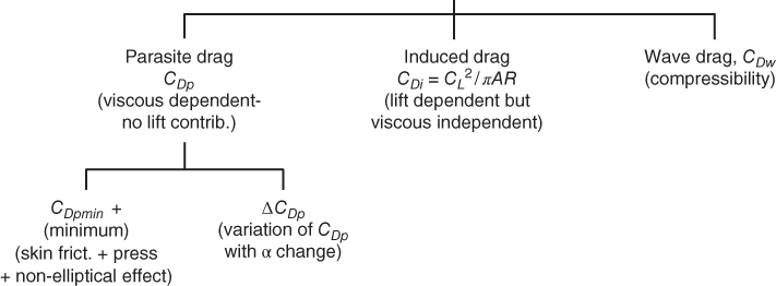
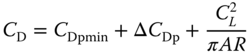
It is apparent that the CD varies with the CL. When the CD and the CL relationship is shown in graphical form, it is known as a drag polar, shown in Figure 11.2 (all components of drag are shown in the figure). The CD versus the CL2 characteristics of Eq. 11.2 are rectilinear, except at high and low CL values (see Figure 11.16 later), because at a high CL (i.e. low speed, high angle of attack), there could be additional drag due to separation; at a very low CL (i.e. high‐speed), there could be additional drag due to local shocks. Both effects are nonlinear in nature. Most of the errors in estimating drag result from computing ΔCDp, three‐dimensional effects, interference effects, excrescence effects of the parasite drag and nonlinear range of aircraft drag. Designers should keep CDw = 0 at LRC and aim to minimise to ΔCDp ≈ 0 (perceived as the design point).

Figure 11.2 Bizjet drag polar (see Section 11.18, Tables 11.13 and 11.16).
An aircraft on a long‐range mission typically can have a weight change of more than 25% from the initial to the final cruise condition. As the aircraft becomes lighter, its induced drag decreases. Therefore, it is more economical to cruise at a higher altitude to take advantage of having less drag. In practical terms, this is achieved in the step‐climb technique, or a gradual climb over the cruise range (Chapter 15).
11.4.1 Discussion
Considering air as inviscid makes mathematics simple to quickly obtain aerodynamic properties of a body in airflow, lift, moment and so on, in the linear range of operation. However, it is incapable to predict drag, stall and so on. In the earlier days aircraft designers had to rely on experimental data and semi‐empirical relations those matured to sufficient accuracy to send man to the Moon.
With advances made in numerical analyses, today, CFD can approximately solve the exact nonlinear partial differential equations to get comparable results to experimental values (Chapter 23 outlines CFD capabilities). However, unlike getting good results on predicting lift and moment characteristics, CFD capability in predicting drag characteristic accurately and consistently has some way to go. This chapter presents industry standard drag predicting methodology, using well substantiated semi‐empirical relationships.
Figure 11.2 plots the Bizjet drag polar and the aircraft components drag values for the Bizjet, as worked out in Section 11.19. It shows that for the Bizjet cruising at Mcrit (LRC at Mach 0.7), about two‐thirds of aircraft drag is viscous dependent, it would exist if air is considered inviscid. There is a small increase in Bizjet drag when flying at Mdiv (HSC at Mach 0.75), on account of a 20 count of wave drag rise (CDW = 0.002, ≈ 6%). These percentages of drag breakdown are a good representation of typical transport aircraft drag.
On examining the aircraft‐component drag breakdown, it can be seen that just the wing and fuselage (with belly fairing and canopy) together contribute to about 60% of the CDPmin. Adding the nacelle drag, together these three components contribute to three‐quarters of the viscous‐dependent parasite drag. Aircraft designers concentrates more on these components to get the best configuration as discussed in Chapters 4–6. Nacelle design is dealt in Section 11.9.3.
11.5 Understanding Drag Polar
Aircraft drag polar is one of the most important information to evaluate aircraft capabilities. To evaluate aircraft performance, a good understanding of drag polar is essential. Aircraft drag polar gives the relation between drag and lift at any instant of flight under consideration. If drag polar could conform to expressing it in a simple analytical form, then it would be easier to obtain close‐form solutions rather quickly and avoid cumbersome computational effort. Engine performance characteristics are not easy to express accurately in analytical form.
11.5.1 Actual Drag Polar
Actual drag polar has the same format as drag polar but not an exact fit to a parabolic equation, especially at low‐ and high‐speed ranges. The methodology for estimating actual drag using semi‐empirical relations is given in this chapter. These semi‐empirical relations are based on experimental data from both wind‐tunnel and flight tests. These are the best available drag polar for industry standard analyses. Drag polar obtained by this methodology is not easily amenable to representation by close‐form equations, especially for high‐subsonic speed aircraft. To generate graphs that fit a parabolic shape, it may require shaping of graphs with the least loss in accuracy. Considerable insight into aircraft performance can be obtained by manipulating the parabolic drag polar equation. The industrial methods presented in this book give all the information but require laborious computational effort.
11.5.2 Parabolic Drag Polar
As mentioned earlier, close‐form solutions from the analytical expressions quickly show important aircraft characteristics and prove useful to make a trend analyses. The readers may refer to [1–4] to study analytical treatments. At LRC, when wave drag is simplified to CDW = 0, then Eq. 11.2 takes the form as follows
where k = 1/eπAR
The difference between the actual aircraft drag polar (CDpmin + ΔCDp + CL2/πAR) and its corresponding parabolic drag polar (CDpmin + kCL2) is in the approximation of the variable lift‐dependent parasite drag ΔCDp to a constant Oswald's efficiency factor ‘e’ associated with the induced drag CDi. The variable parameter ‘e’ is approximated to a constant value bringing parabolic drag polar close to actual drag polar around the cruise segment and also gives a good match at climb and descent segments.
Figure 11.3 shows the variation of Oswald's efficiency factor ‘e’ with Mach number for the Bizjet aircraft at 18 000 lb weight cruising at a 41 000 ft altitude (CL ≈ 0.512). It is evaluated using the following equation and plotted in the figure.

Figure 11.3 Bizjet Oswald's efficiency factor ‘e’ variation at 41 000 ft altitude (18 000 lb weight, CL ≈ 0.512, AR = 7.5).
where e = (1/kπAR)
Parabolic drag polar incorporates a value of k = 0.0447 (e ≈ 0.95) representing average values. At the design CL (typically, at mid‐LRC) it approaches 1. This will cause a discrepancy between parabolic drag polar and actual drag polar values at higher speeds. For flying close to the ground, low speed incorporates drag of a ‘dirty configuration’ with values accommodating changes in e. For this reason, this book suggests that, for high‐subsonic aircraft, one should use actual drag polar for accurate industry standard results, for example, for certification substantiation, preparing the pilot manual and so on, and parabolic drag polar may be used for exploring and establishing aircraft characteristics.
11.5.3 Comparison Between Actual and Parabolic Drag Polar
The parabolic representation of aircraft drag polar offers many advantages. Easy mathematical manipulation gives a quick insight to aircraft characteristics at an early design phase to make improvements, if required. Industry needs drag prediction to be as accurate as possible (in the order of few counts) and, therefore, results from approximate analytical expression are not adequate for high‐subsonic aircraft, especially when good prediction of drag polar can be obtained through semi‐empirical relations substantiated by testing.
This section attempts to present approximated analytical expression for high‐subsonic aircraft drag polar. Recall Eq. 11.2, which gives the expression for high‐subsonic aircraft drag as
where (CDpmin + CL2/πAR) represents parabola in which CDpmin is the minimum distance of the drag polar from the y‐axis representing CL.
Equation 11.4 is not exactly of parabolic shape, depending on the extent to which it is contributed to by the non‐parabolic component of ΔCDp and the wave drag term CDW. In an incompressible flow regime CDW drops out and ΔCDp is integrated with the induced drag term with the suitable coefficient ‘k’ = 1/eπ AR (where e is the Oswald's efficiency factor) to represent the parabola equation as discussed before. A carefully designed aircraft can have ΔCDp ≈ 0 at cruise CL. The simplification brings Eq. 11.4 into a simpler form as in Eq. 11.5, making it easier to handle.
This form of representation can be applied to high‐speed subsonic aircraft up to LRC, that is, up to Mcrit. When the parabolic part of the CD is plotted against CL2, it is a straight line (Figure 11.16b).
Equation 11.5 can be improved by modifying to more accurate form as shown in Eq. 11.6 (plotted in Figure 11.4a).

Figure 11.4 Bizjet comparison example. (a) Analytical (parabolic) and semi‐empirical drag polar comparison. (b) Drag comparison.
where CDpmin is at CLm and not at CL = 0.
In the generalised situation of high‐speed subsonic aircraft, CDpmin is not necessarily at CL = 0. Figure 11.4 typically represents Eqs. 11.4 and 11.5 with drag polar estimated by a semi‐empirical method (as done in Table 11.16 later). The various CL points shown in the graph appear in analytical equations derived in the subsequent sections using the parabolic drag Eq. 11.3.
(The most generalised form of aircraft drag polar can be expressed in a polynomial expression as given in Eq. (11.7).
For high‐subsonic aircraft, terms above k3CL3 contribute very little and can be ignored. Even then, the polynomial form is not amenable to an easy close‐form solution. The supersonic drag expression can be dealt with using a similar rationale (and its details are not dealt with here).
The expression for parabolic drag polar as given in Eq. 11.5 is
where k = 1/eπAR
Figure 11.4a presents an analytical comparison between actual drag polar with parabolic drag polar. It may be noted that the three graphs are close enough within the operating range below Mcrit. Figure 11.4b presents the Bizjet example as worked out in Section 11.19. Section 11.4 represents a typical high speed subsonic aircraft operational segments of an LRC (when CDW = 0), en‐route climb and descent. At HSC, the non‐linear effects show up. The Bizjet operates in high subsonic speeds at Mcrit and, therefore, semi‐empirically determined actual drag polar is the preferred one. This is the standard procedure as practiced in industry, which gives credible output.
11.6 Aircraft Drag Formulation
A theoretical overview of drag is provided in this section to show that aircraft geometry is not amenable to the equation for an explicit solution. Even so, CFD is yet to achieve an acceptable result for the full aircraft.
Recall the expression in Eq. 11.2 for the total aircraft drag, CD, as:
where CDparasite = CDfriction + CDpressure = CDpmin + ΔCDp.
At LRC, when CDw ≈ 0, the total aircraft drag coefficient is given by:
The general theory of drag on a 2D body (Figure 11.5a) provides the closed‐form Eq. (11.11a). A 2D body has an infinite span. In the diagram, airflow is along the x direction and wake depth is shown in the y direction. The wake is formed due to viscous effects immediately behind the body, where integral operation is applied. Wake behind a body is due to the viscous effect in which there is a loss of velocity (i.e. momentum) and pressure (depletion of energy) as shown in the figure. Measurement and computation across the wake are performed close to the body; otherwise, the downstream viscous effect dissipates the wake profile. Consider an arbitrary control volume (CV) large enough in the y direction where static pressure is equal to free‐stream static pressure (i.e. p = p∞). The subscript ∞ denotes the free‐stream condition. Integration over the y direction on both sides up to the free‐stream value gives.

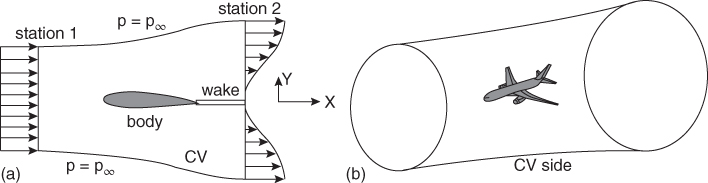
Figure 11.5 Control volume (CV) approach to formulate aircraft drag: (a) 2D body and wake in CV and (b) 3D aircraft in CV.
An aircraft is a 3D object (Figure 11.5b) with the additional effect of finite wing span that will produce induced drag. In that case, Eq. (11.11a) can be written as
where b is the span of the wing in the x direction (the axis system has changed).
The finite wing effects on the pressure and velocity distributions result in induced drag Di embedded in the expression on the right‐hand side of Eq. (11.11b). Because the aircraft cruise condition (i.e. LRC) is chosen to operate below the onset of wave drag at Mcrit, the wave drag, Dw, is absent; otherwise, it must be added to the expression. Therefore, Eq. (11.11b) can be equated with the aircraft drag expression as given in Eq. 11.9. Finally, Eq. (11.11b) can be expressed in a non‐dimensional form, by dividing ½ρ∞U∞2SW. Therefore

Unfortunately, the complex 3D geometry of an entire aircraft in Eq. 11.12 is not amenable to easy integration. CFD has discretised the flow field into small domains that are numerically integrated, resulting in some errors. Mathematicians have successfully managed the error level with sophisticated algorithms. The proven industrial‐standard, semi‐empirical methods are currently the prevailing practice and are backed up by theories and validated by flight tests. CFD assists in the search for improved aerodynamics.
11.7 Aircraft Drag Estimation Methodology (Subsonic)
The semi‐empirical formulation of aircraft drag estimation used in this book is a credible method based on [1, 3, 7, 8]. It follows the findings from NACA/NASA, RAE and other research‐establishment documents. This chapter provides an outline of the method used. It is clear from Eq. 11.2 that the following four components of aircraft drag are to be estimated:
- Minimum parasite drag, CDpmin (see Section 11.9).
Parasite drag is composed of skin friction and pressure differences due to viscous effects that are dependent on the Re. To estimate the minimum parasitic drag, CDpmin, the first task is to establish geometric parameters such as the characteristic lengths and wetted areas and the Re of the discrete aircraft components.
- Incremental parasite drag, ΔCDp (see Section 11.9).
CDp is a characteristic of a particular aircraft design and includes the lift‐dependent parasite drag variation, 3D effects, interference effects and other spurious effects not easily accounted for. There is no theory to estimate ΔCDp; it is best obtained from wind‐tunnel tests or the ΔCDp of similarly designed aircraft wings and bodies. CFD results are helpful in generating the CDp‐versus‐CL variation.
- Induced drag, CDi (see Section 4.18).
The pure induced drag, CDi, is computed from the expression
11.13
- Wave drag, CDw (see Section 11.13).
The last component of subsonic aircraft drag is the wave drag, CDw, which accounts for compressibility effects. It depends on the thickness parameter of the body: for lifting surfaces it is the t/c ratio, and for bodies it is the diameter‐to‐length ratio. CFD can predict wave drag accurately but must be substantiated using wind‐tunnel tests. Transport aircraft are designed so that HSC at Mcrit (e.g. 320 type, ≈ 0.82 Mach) allows a 20‐count (CDw = 0.002) drag increase. At LRC, wave drag formation is kept at zero. Compressibility drag at supersonic speed is caused by shock waves.
The methodology presented herein considers fully turbulent flow from the leading edge (LE) of all components. Here, no credit is taken for drag reduction due to possible laminar flow over a portion of the body and lifting surface. This is because it may not always be possible to keep the aircraft surfaces clear of contamination that would trigger turbulent flow. The certifying agencies recommend this conservative approach.
11.8 Minimum Parasite Drag Estimation Methodology
The practised method of computing CDpmin is first to dissect (i.e. isolate) the aircraft into discrete identifiable components, such as the fuselage, wing, V‐tail, H‐tail, nacelle and other smaller geometries (e.g. winglets and ventral fins). The wetted area and the Re of each component establish skin friction associated with each component. The 2D flat plate basic means the skin friction coefficient, CF_basic, corresponding to the Re of the component, is determined from Figure 11.24, bottom graph for the flight Mach number. Section 11.19.1 explains the worked‐out examples carried out in this book for fully turbulent flow.
The CFs arising from the 3D effects (e.g. supervelocity) and wrapping effects of the components are added to the basic flat plate CF_basic. Supervelocity effects result from the 3D nature (i.e. curvature) of aircraft‐body geometry where, in the critical areas, the local velocity exceeds the free‐stream velocity (hence the term supervelocity). The axi‐symmetric curvature of a body (e.g. fuselage) is perceived as a wrapping effect when the increased adverse pressure gradient increases the drag. The interference in the flow field is caused by the presence of two bodies in proximity (e.g. the fuselage and wing). The flow field of one body interferes with the flow field of the other body, causing more drag. Interference drag must be accounted for when considering the drag of adjacent bodies or components – it must not be duplicated while estimating the drag of the other body.
The design of an aircraft should be streamlined so that there is little separation over the entire body, thereby minimising parasite drag obtained by taking the total CF (by adding various CF, to CF_basic). Hereafter, the total CF will be known as the CF. Parasite drag is converted to its flat plate equivalent expressed in ‘f’ square feet. In this book, the FPS system is used for comparison with the significant existing data that use the FPS system, although it can be easily converted into the international system of units (SI) system. Being non‐dimensional, working in SI will give the same value of drag coefficients. The flat plate equivalent ‘f’ is defined as:
where Aw is the wetted area (unit in ft2).
The minimum parasite drag CDpmin of an aircraft is obtained by totalling the contributing fs of all aircraft components with other sundries. Therefore, the minimum parasite drag of the aircraft is obtained by:
The stepwise approach to computing CDpmin is described in the following three subsections.
11.8.1 Geometric Parameters, Reynolds Number and Basic CF Determination
The Re (= (ρ∞LcompV∞)/μ∞) has the deciding role in determining the skin friction coefficient, CF, of a component. First, the Re per unit length, speed and altitude are established. Then, the characteristic lengths of each component are determined. The characteristic length Lcomp of each component is as follows.
- Fuselage. Axial length from the tip of the nose cone to the end of the tail cone (Lfus)
- Wing. The wing Mean Aerodynamic Chord (MAC)
- Empennage. The MACs of the V‐tail and the H‐tail
- Nacelle. Axial length from the nacelle highlight plane to the nozzle‐exit plane (Lnac)
Figure 11.24 shows the basic 2D flat plate skin friction coefficient of a fully turbulent flow for local (Cf_basic) and average (CF_basic) values. For a partial laminar flow, the CF_basic correction is made using factor f1, given in Figure 11.25. It has been shown that the compressibility effect increases the boundary layer, thus reducing the local CF. However, in LRC until the Mcrit is reached, there is little sensitivity of the CF change with Mach number variations, therefore, the incompressible CF line (i.e. the Mach 0 line in Figure 11.24 (bottom graph) is used. At HSC at the Mcrit and above, the appropriate Mach line is used to account for the compressibility effect. The basic CF changes with changes in the Re, which depends on speed and altitude of the aircraft. Section 11.2 explains that a subsonic aircraft CDpmin computed at LRC would cater to the full flight envelope, in this book. For HSC, the wave drag ΔCDw is to be added.
11.8.2 Computation of Wetted Areas
Computation of the wetted area, Aw, of the aircraft component is shown herein. Skin friction is generated on that part of the surface over which air flows, the so‐called wetted area. Wetted area Aw computation has to be accurate as parasite drag is directly proportionate to Aw. A 2% error in area estimation will result in about 1% error in overall subsonic aircraft drag.
Three‐dimensional computer aided drawing (CAD) model can give accurate wetted area, Aw. In case CAD data are not available, the component wetted areas can be estimated from manually drawn three‐view diagram in a large sheet (say A0 or A1 size) by draftsmen in a different department and then given to aerodynamics group where drag estimation is done. Planimeters prove useful in making accurate area measurements. Normally, three‐view 2D drawings have the reference areas of the geometry that can help calibrating the planimeter in use.
11.8.2.1 Lifting Surfaces
These are approximate to the flat surfaces, with the wetted area slightly more than twice the reference area due to some thickness. Care is needed in removing the areas at intersections, such as the wing area buried in the fuselage. A factor k is used to obtain the wetted area of lifting surfaces, as follows:
Aw = k × (exposed reference area, SW; the area buried in the body is not included). The factor k may be interpolated linearly for other t/c ratios.
where k = 2.02 for t/c = 0.08%
- = 2.04 for t/c = 0.12%
- = 2.06 for t/c = 0.16%
11.8.2.2 Fuselage
The fuselage is conveniently divided into sections – typically, for a civil transport aircraft, into a constant cross‐section mid‐fuselage with varying cross‐section front and aft‐fuselage closures. The constant cross‐section mid‐fuselage barrel has a wetted area of Awfmid = perimeter × length. The forward‐ and aft‐closure cones could be sectioned more finely, treating each thin section as a constant section ‘slice’. A military aircraft is unlikely to have a constant cross‐section barrel and its wetted area must be computed in this way. The wetted areas must be excluded where the wing and empennage join the fuselage or for any other considerations.
11.8.2.3 Nacelle
Only the external surface of the nacelle is considered the wetted area and it is computed in the same way as the fuselage, taking note of the pylon cut‐out area. (Internal drag within the intake duct is accounted for as installation effects in engine performance as a loss of thrust.)
11.8.3 Stepwise Approach to Compute Minimum Parasite Drag
The following seven steps are carried out to estimate the minimum parasite drag, CDpmin:
- Step 1. Dissect and isolate aircraft components such as wing, fuselage nacelle and so on. Determine the geometric parameters of the aircraft components such as the characteristic length and wetted areas.
- Step 2. Compute Re per foot at the LRC condition. Then obtain the component Re by multiplying its characteristic length.
- Step 3. Determine the basic 2D (Figure 11.24, bottom graph) average skin friction coefficient CF_basic, corresponding to the Re for each component.
- Step 4. Estimate the ΔCF as the increment on account of 3D effects on each component.
- Step 5. Estimate the interference drag of two adjacent components. Avoid duplication.
- Step 6. Add results obtained in steps 3–5 to get the minimum parasite drag of the component in terms of flat plate equivalent area (ft2 or m2); that is, CF = CF_2D + ∑ΔCF for the component. ( f)comp = (Aw)comp × CF, where (CDpmin)comp = ( f)comp/Sw.
- Step 7. Add all the component minimum parasite drags. Then add other drags, for example, trim excrescence drag and so on. Finally, add 3% drag due to surface roughness effects. The aircraft minimum parasite drag is expressed in coefficient form, CDpmin.
The semi‐empirical formulation for each component is given in the following subsections.
11.9 Semi‐Empirical Relations to Estimate Aircraft‐Component Parasite Drag
Isolated aircraft components are worked on to estimate component parasite drag. The semi‐empirical relations given here embed the necessary corrections required for 3D effects. Associated coefficients and indices are derived from actual flight‐test data. (Wind‐tunnel tests are conducted at a lower Re and therefore require correction to represent flight‐tested results.) The influence of the related drivers is shown as drag increasing by ↑ and drag decreasing by ↓. For example, an increase of the Re reduces the skin friction coefficient and is shown as Re (↓).
11.9.1 Fuselage
The fuselage characteristic length, Lfus, is the length from the tip of the nose cone to the end of the tail cone. The wetted area, Awf (↑), and fineness ratio (length/diameter) (↓) of the fuselage are computed. Ensure that cut‐outs at the wing and empennage junctions are subtracted. Obtain the Ref (↓). The corresponding basic CFf for the fuselage using (Figure 11.24. bottom graph) is intended for the flat plate at the flight Mach number. Figure 11.24 is accurate and validated over time.
The methodology for the fuselage (denoted by the subscript f) is discussed in this section. The Ref is calculated first using the fuselage length as the characteristic length. The semi‐empirical formulation is required to correct the 2D skin friction drag for the 3D effects and other influencing parameters, as listed herein. These are incremental values shown by the symbol Δ. There are many incremental effects and it is easy to miss some of them.
- 3D effects [1]: 3D effects are on account of surface curvature resulting in change in local flow speed and associated pressure gradients:
- (i) Wrapping:
11.16where k is between 0.022 and 0.025 (take the higher value) and Re = Reynolds Number of fuselage

- (ii)
Supervelocity:
11.17

- (iii)
Pressure:
11.18

- (i) Wrapping:
- Other effects on the fuselage (increments are given as a percentage of 2D CFf) are listed herein. The industry has more accurate values of these incremental ΔCFf. Readers in the industry should not use the values given here – they are intended only for coursework using estimates extracted from industrial data.
- (i)
Canopy drag. There are two types of canopy (Figure 11.6), as follows:
- 1. Raised or bubble‐type canopy or its variants. These canopies are mostly associated with military aircraft and smaller aircraft. The canopy drag coefficient CDπ is based on the frontal cross‐sectional area shown in the military‐type aircraft in Figure 11.6 (the front view of the raised canopy is shaded). The extent of the raised frontal area contributes to the extent of drag increment and the CDπ accounts for the effects of canopy rise. CDπ is then converted to CFfcanopy = (Aπ × CDπ)/Awf, where Awf is the fuselage wetted area. The dominant types of a raised or bubble‐type canopy and their associated CDπ are summarised in Table 11.1.
- 2. Windshield‐type canopy for larger aircraft. These canopies are typically associated with payload‐carrying commercial aircraft from a small Bizjet and larger. Flat panes lower the manufacturing cost but result in a kink at the double curvature nose cone of the fuselage. A curved and smooth transparent windshield avoids the kink that would reduce drag at an additional cost. Smoother types have curved panes with a single or double curvature. Single‐curvature panes come in smaller pieces, with a straight side and a curved side. Double curvature panes are the most expensive and considerable attention is required during manufacturing to avoid distortion of vision. The values in square feet in Table 11.2 are used to obtain a sharp‐edged windshield‐type canopy drag.
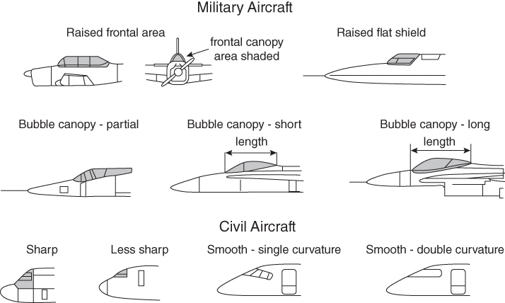
Figure 11.6 Canopy types for drag estimation. Table 11.1 Typical CDπ associated with raised or bubble‐type canopies. Raised frontal area (older boxy design – has sharp edges) CDπ = 0.2 Raised flat shield (reduced sharp edges) CDπ = 0.15 Bubble canopy (partial) CDπ = 0.12 Bubble canopy (short) CDπ = 0.08 Bubble canopy (long) CDπ = 0.06 Adjust the values for the following variations. Kinked windshield (less sharp) reduce the value by 10% Smoothed (single‐curvature) windshield reduce the value by 20–30% Smoothed (double‐curvature) windshield reduce the value by 30–50%
- (ii) Body pressurisation – fuselage surface waviness, 4–6%
- (iii)
Non‐optimum fuselage shape (interpolate the in‐between values)
- 1.
Front fuselage closure ratio, Fcf (see Section 5.4.3)
- For Fcf ≤ 1.5: 8%
- For 1.5 ≤ Fcf ≤ 1.75: 6%
- For Fcf ≥ 1.75: 4%
- For military aircraft type with high nose fineness: 3%
- 2.
Aft fuselage closure angle, (see Section 5.4.3)
- Less than 10°: 0
- 11–12° closure: 1%
- 13–14°: 4%
- 3.
Upsweep closure (see Section 5.4.3) use in conjunction with (4)
- No upsweep: 0
- 4° of upsweep: 0–2%
- 10° of upsweep: 4–8%
- 15° of upsweep: 10–15%
- (interpolate in‐between values)
- 4.
Aft‐end cross‐sectional shape
- Circular: 0
- Shallow keel: 0–1%
- Deep keel: 1–2%
- 5. Rear‐mounted door (with fuselage upsweep): 5–10%
- 1.
Front fuselage closure ratio, Fcf (see Section 5.4.3)
- (iv) Cabin‐pressurisation leakage (if unknown, use higher value): 2–5%
- (v)
Excrescence (non‐manufacturing types such as windows)
- Windows and doors (use higher values for larger aircraft): 2–4%
- Miscellaneous: 1%
- (vi) Wing‐fuselage belly fairing, if any: 1–5% (use higher value if houses undercarriage)
- (vii) Undercarriage fairing – typically for high‐wing aircraft (if any fairing): 2–6% (based on fairing protrusion height from fuselage)
- (i)
Canopy drag. There are two types of canopy (Figure 11.6), as follows:
- The interference drag increment with the wing and empennage is included in the calculation of lifting‐surface drag and therefore is not duplicated when computing the fuselage parasite drag. Totalling the CFf and ΔCFf from the wetted area Awf of the isolated fuselage, the flat plate equivalent drag, ffus (see Step 6 in Section 11.8.3), is estimated in square feet.
- Surface roughness is 2–3%. These effects are from the manufacturing origin, discussed in Section .
Table 11.2 Typical CDπ associated with sharp wind shield type canopies (drag in sq. ft).
| 2‐abreast seating aircraft | 0.1 sq. ft | 8‐abreast seating aircraft | 0.4 sq. ft |
| 4‐abreast seating aircraft | 0.2 sq. ft | 10‐abreast or more | 0.5 sq. ft |
| 6‐abreast seating aircraft | 0.3 sq. ft |
Total all the components of parasite drag to obtain CDpmin, as follows. It should include the excrescence drag increment. Converted into the fuselage contribution to [CDpmin]f in terms of aircraft wing area, it becomes:
Because surface roughness drag is the same percentage for all components, it is convenient to total them after evaluating all components. In that case, the term ΔCFf_rough is dropped from Eq. 11.20.
11.9.2 Wing, Empennage, Pylons and Winglets
The wing, empennage, pylon and winglets are treated as lifting surfaces and use identical methodology to estimate their minimum parasite drag. It is similar to the fuselage methodology except that it does not have the wrapping effect. Here, the interference drag with the joining body (e.g. for the wing, it is the fuselage) is taken into account because it is not included in the fuselage ffus.
The methodology for the wing (denoted by the subscript w) is discussed in this section. The Rew is calculated first using the wing MAC as the characteristic length. Next, the exposed wing area is computed by subtracting the portion buried in the fuselage and then the wetted area, AWw, using the k factors for the t/c as in Section 11.8.2.1. Using the Rew, the basic CFw_basic is obtained from the graph in Figure 11.24, bottom graph for the flight Mach number. The incremental parasite drag formulae are as follows:
- 3D effects (taken from [1]):
- Supervelocity:
11.22where K1 = 1.2–1.5 for supercritical aerofoil

K1 = 1.6–2 for conventional aerofoil
- Pressure:
11.23

where aspect ratio AR ≥ 2 (modified from [1])
Last term of this expression includes the effect of non‐elliptical lift distribution.
- Supervelocity:
- Interference:
11.24
where K2 = 0.6 for high and low wing designs and CB is the root chord at fuselage intersection. For mid‐wing, K2 = 1.2. This is valid for t/c ratio > 0.07. For a t/c ratio below 0.07, take the interference drag
11.25
- The same relations apply for the V‐tail and H‐tail.
- For pylon interference 10–12%
- Interference drag is not accounted for in fuselage drag, it is accounted for in wing drag.
- (For the pylon, one interference is at the aircraft side and one is with the nacelle.)
- Other effects:
- Excrescence (non‐manufacturing, e.g. control surface gaps etc.):
Flap gaps 4–5% Slat gaps 4–5% Others 4–5% - Surface roughness (to be added later)
The flat plate equivalent of wing drag contribution is (subscript is self‐explanatory)
which can be converted into CDpmin in terms of aircraft wing area
(Drop the term ΔCFwrough of Eq. 11.20 if it is accounted for at the end after computing fs for all components as shown in Eq. 11.28.)
The same procedure is used to compute the parasite drag of empennage, pylons and so on, which are considered as being wing‐like lifting surfaces.
which can be converted into
As before, it is convenient to total ΔCFfrough after evaluating all components. In that case, the term ΔCFfrough is dropped from Eq. 11.20 and it is accounted for as shown in Eq. 11.21.
11.9.3 Nacelle Drag
The nacelle requires different treatment, with the special consideration of throttle dependent air flowing through as well as over it, like the fuselage. This section provides the definitions and other considerations needed to estimate nacelle parasite drag (see [2, 9, 15, 16]). The nacelle is described in Section 5.12.
The throttle dependent variable of the internal flow passing through the turbofan engine affects the external flow over the nacelle. The dominant changes in the flow field due to throttle dependency are around the nacelle at the lip and aft end. When the flow field around the nacelle is known, the parasite drag estimation method for the nacelle is the same as for the other components but must also consider the throttle dependent effects.
Civil aircraft nacelles are typically pod‐mounted. In this book, only the long duct is considered. Military aircraft engines are generally buried in the aircraft shell (i.e. fuselage). A podded nacelle may be thought of as a wrapped‐around wing in an axi‐symmetric shape like that of a fuselage. The nacelle section shows aerofoil‐like sections in Figure 11.7; the important sources of nacelle drag are listed here (a short duct nacelle (see Figure 12.17) is similar except for the fan exhaust coming out at high‐speed over the exposed outer surface of the core nozzle, for which its skin friction must be considered):
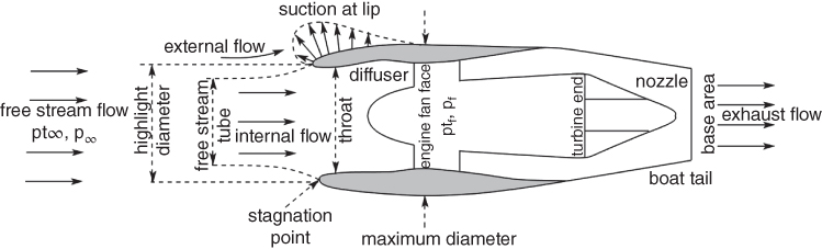
Figure 11.7 Aerodynamic considerations for an isolated long‐duct nacelle drag.
Nacelles do not have front fuselage like curvature and aft fuselage like upsweep curvatures. Nacelle external flow is throttle dependent and is affected by the internal intake flow when the lip suction effect (Figure 11.7) is considered. Nacelle aft has little separation with the exhaust flow entrainment effect and boat tail (see next) drag takes into account of the pressure drag. Therefore, unlike fuselage drag considerations, the supervelocity and pressure effects are not considered in case of nacelle drag estimation.
- Throttle‐independent drag (external surface) – at cruise thrust
- skin friction
- wrapping effects of axi‐symmetric body excrescence effects (includes non‐manufacturing types such as cooling ducts.)
- Throttle dependent drag
- inlet drag (front end of the diffuser)
- nacelle base drag (zero for an engine operating at cruise settings and higher)
- boat tail drag (curvature of the nozzle at the aft end of the nacelle)
Definitions and typical considerations for drag estimation associated with flow field around an isolated long‐duct podded nacelle (approximated to circular cross‐section) are shown in Figure 11.7. Although there is internal flow through the nacelle, the external geometry of the nacelle may be treated as a fuselage, except that there is a lip section similar to the LE of an aerofoil. The prevailing engine throttle setting is maintained at a rating for LRC or HSC for the mission profile. The intake drag and the base drag/boat tail drag are explained next.
11.9.3.1 Intake Drag
The intake stream tube flow pattern at cruise is complex that makes intake drag estimation difficult (Figure 11.7). There is spillage during the subcritical operation due to the stream tube being smaller than the cross‐sectional area at the nacelle highlight diameter, where external flow turns around the lip creating suction (i.e. thrust). This develops pre‐compression, ahead of the intake, when the intake velocity is slower compared to the free‐stream velocity expressed in the fraction (Vintake/V∞). At (Vintake/V∞) < 0.8. The excess air flow spills over the nacelle lip. The intake lip acts as the LE of a circular aerofoil. The subcritical air flow diffusion ahead of the inlet results in pre‐entry drag called additive drag. The net effect results in spillage drag, as described herein. The spillage drag added to the friction drag at the lip results in the intake drag, which is a form of parasite drag. (For the military aircraft intake, see Sections 12.8.2 and 5.16.1.)
intake drag = spillage drag + friction drag at the lip (supervelocity effect).
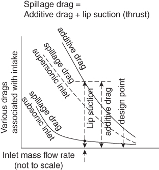
Figure 11.8 Throttle dependent spillage drag (subsonic case shown).
Section 11.8 shows intake drag variations with the mass flow rate for both subsonic and supersonic (i.e. sharp LE) intake.

Figure 11.9 Wing and fuselage‐mounted nacelle.
11.9.3.2 Base Drag
The design criteria for the nozzle exit area sizing is such that at LRC, the exit plane static pressure Pe equals the ambient pressure P∞ (a perfectly expanded nozzle, Pe = P∞) to eliminate any base drag. At higher throttle settings, when Pe > P∞, there still is no base drag. At lower settings, for example, idle rating – there is some base drag as a result of the nozzle exit area being larger than what is required.
11.9.3.3 Boat Tail Drag
The long‐duct contour for closure (i.e. ‘boat tail’ shape) at the aft end is shallow enough to avoid separation, especially with the assistance of entrainment effects of the exhaust plume. Hence, the boat tail drag is kept low. At the idle throttle setting, considerable flow separation can occur and the magnitude of boat tail drag would be higher, but it is still small compared to the nacelle drag.
For book‐keeping purposes and to avoid conflict with aircraft manufacturers, engine manufacturers generally include internal drag (e.g. ram, diffuser and exhaust‐pipe drag) in computing the net thrust of an engine. Therefore, this book only needs to estimate the parasite drag (i.e. external drag) of the nacelle. Intake duct loss is considered engine installation losses expressed as intake‐recovery loss. Intake‐ and exhaust‐duct losses are approximately 1–3% in engine thrust at LRC (throttle and altitude dependent). The net thrust of the turbofan, incorporating installation losses, is computed using the engine‐manufacturer‐supplied programme and data. These manufacturers work in close liaison to develop the internal contour of the nacelle and intake. External nacelle‐contour design and airframe integration remain the responsibility as the aircraft manufacturer.
11.9.3.4 Nacelle 3D Effects
The long‐duct nacelle characteristic length, Lnac, is the length measured from the intake‐highlight plane to the exit area plane. The wetted area AWn, Re and basic CFn are estimated as for other components. The incremental parasite drag formulae for the nacelle are provided herein. The supervelocity effect around the nacelle lip section is included in the intake drag estimation; hence, it is not computed separately. Similarly, the pressure effect is included in the base/boat tail drag estimation. These two items are addressed this way because of the special consideration of throttle dependency. The following are the relationships used to compute the nacelle drag coefficient CDn. The stepwise approach to compute this is:
- 11.31

- (i) Wrapping: ΔCFn = 0.025 × (diameter/length)−1 × Re−0.2
- Other incremental effects.
Drag contributions made by the following effects are given as a percentage of CFn. These are typical of the generic nacelle design.
- (i) Intake drag at LRC – includes supervelocity effects ≈ 40–60% (higher bypass ratio having higher percent)
- (ii) Boat Tail/Base drag (throttle dependent) – includes pressure effects ≈ 10–12% (higher value for smaller aircraft)
- (iii) Excrescence (non‐manufacturing type, e.g. cooling air intakes etc.) ≈ 20–25% (higher value for smaller aircraft)
- Interference drag – a podded nacelle in the vicinity of wing or body would have interference drag as follows (per nacelle). For a wing‐mounted nacelle, the higher the overhang forward of the wing, the lower the interference drag.
Typical values of the interference drag by the pylon (each) interacting with the wing or the body) are given in Table 11.3.
- Surface roughness (add later ≈ 3%)
Table 11.3 Nacelle interference drag (per nacelle).
| Wing mounted (Figure 11.9) | Fuselage mounted (Figure 11.9) | ||
| Interference drag | Interference drag | ||
| High (long) overhang | 0 | Raised | 5% of CFn |
| Medium overhang | 4% of CFn | Medium | 5% of CFn |
| Low (short) overhang | 7% of CFn | Low | 5% of CFn |
| S‐duct | 6.5% of CFn | ||
| Straight duct (centre) | 5.8% of CFn | ||
A long overhang in front of the wing keeps the nacelle free from interference effects, a short overhang has the highest interference. However, there is little variation of inference drag of nacelle mounted on different position at the aft fuselage. Much depends on the proximity of other bodies, for example, wing, empennage and so on. If the nacelle is within one diameter, then interference drag may be increased by another 0.5%. The centre engine is close to fuselage and with V‐tail – they have increased interference.
11.9.3.5 Total Nacelle Drag
By adding all the components, the flat plate equivalent of nacelle drag contribution is given by Eq. 11.32.
As before, it is convenient to total ΔCFfrough after evaluating all components. In that case, the term ΔCF_rough is dropped from Eq. 11.32 and it is accounted for as shown in Eq. 11.34. Converted into the nacelle contribution to CDpmin in terms of aircraft wing area it becomes
In the last three decades, the nacelle drag has been reduced by approximately twice as much as what has been achieved to other aircraft components. This demonstrates the complexity of and unknowns associated with the flow field around nacelles. CFD is important in nacelle design and its integration with aircraft. In this book, nacelle geometry is simplified to the axi‐symmetric shape without loss of methodology.
11.9.4 Recovery Factor
Intake duct loss will deplete some flow energy making fan face total pressure, Ptf, less than free‐stream total pressure, Pt∞. The extent of total loss is expressed as the recovery factor, RF. Thrust loss on account of RF is seen as installation loss and is accounted in installed engine thrust and is dealt in Section 13.2.1.
11.9.5 Excrescence Drag
An aircraft body is not smooth; located all over the body are probes, blisters, bumps, protrusions, surface‐protection mats for steps, small ducts (e.g. for cooling) and exhausts (e.g. environmental control and cooling air) – these are unavoidable features. In addition, there are mismatches at subassembly joints – for example, steps, gaps and waviness originating during manufacture and treated as discreet roughness. Pressurisation also causes the fuselage‐skin waviness (i.e. areas ballooning up). In this book, excrescence drag is addressed separately as two types:
1. Manufacturing origin [16]. This includes aerodynamic mismatches as discreet roughness resulting from tolerance allocation. Aerodynamicists must specify surface smoothness requirements to minimise excrescence drag resulting from the discrete roughness, within the manufacturing‐tolerance allocation.
2. Non‐manufacturing origin. This includes aerials, flap tracks and gaps, cooling ducts and exhausts, bumps, blisters and protrusions.
Excrescence drag due to surface roughness drag is accounted for by using 2–3% of component parasite drag as roughness drag ([1, 7]). As indicated in Step 7 of Section 11.8.3, fcomp total is increased by 3% using a factor of 1.03 after computing all component parasite drags, as follows
The difficulty in understanding the physics of excrescence drag was summarised by Haines [12] in his review by stating ‘…one realises that the analysis of some of these early data seems somewhat confused, because three major factors controlling the level of drag were not immediately recognised as being separate effects’. These factors are as follows:
- how skin friction is affected by the position of the boundary‐layer transition
- how surface roughness affects skin friction in a fully turbulent flow
- how geometric shape (non‐planar) affects skin friction
Haines's study showed that a small but significant amount of excrescence drag results from manufacturing origin and was difficult to understand.
11.9.6 Miscellaneous Parasite Drags
In addition to excrescence drag, there are other drag increments such as from the intake drag of the environmental control system (ECS) (e.g. air‐conditioning), which is a fixed value depending on the number of passengers) and aerials and trim drag, which are included to obtain the minimum parasite drag of the aircraft.
11.9.6.1 Air‐Conditioning Drag
Air‐conditioning air is inhaled from the atmosphere through flush intakes that incur drag. It is mixed with hot air bled from a mid‐stage of the engine compressor and then purified. Loss of thrust due to engine bleed is accounted for in the engine thrust computation, but the higher pressure of the expunged cabin air causes a small amount of thrust. Table 11.4 shows the air‐conditioning drag based on the number of passengers (interpolation is used for the between sizes).
Table 11.4 Air‐conditioning drag.
| No. of passengers | Drag – f (ft2) | Thrust – f (ft2) | Net drag – f (ft2) |
| 50 | 0.1 | −0.04 | 0.06 |
| 100 | 0.2 | −0.1 | 0.1 |
| 200 | 0.5 | −0.2 | 0.4 |
| 300 | 0.8 | −0.3 | 0.5 |
| 600 | 1.6 | −0.6 | 1.0 |
11.9.6.2 Trim Drag
Due to weight changes during cruise, the centre of gravity (CG) could shift, thereby requiring the aircraft to be trimmed in order to relieve the control forces. Change in the trim‐surface angle causes a drag increment. The average trim drag during cruise is approximated as shown in Table 11.5, based on the wing reference area (interpolation is used for the between sizes).
Table 11.5 Trim drag (approximate).
| Wing reference area (ft2) | Trim drag f (ft2) | Wing reference area (ft2) | Trim drag – f (ft2) |
| 200 | 0.12 | 2000 | 0.3 |
| 500 | 0.15 | 3000 | 0.5 |
| 1000 | 0.2 | 4000 | 0.8 |
11.9.6.3 Aerials
Navigational and communication systems require aerials that extend from an aircraft body, generating parasite drag on the order 0.06–0.1 ft2, depending on the size and number of aerials installed. For midsized transport aircraft, 0.075 ft2 is typically used. Therefore:
11.10 Notes on Excrescence Drag Resulting from Surface Imperfections
Excrescence drag due to surface imperfections is difficult to estimate; therefore, this section provides background on the nature of the difficulty encountered. Capturing all the excrescence effects over the full aircraft in CFD is yet to be accomplished with guaranteed accuracy.
A major difficulty arises in assessing the drag of small items attached to the aircraft surface, such as instruments (e.g. pitot and vanes), ducts (e.g. cooling) and necessary gaps to accommodate moving surfaces. In addition, there is the unavoidable discrete surface roughness from mismatches and imperfections – aerodynamic defects – resulting from limitations in the manufacturing processes. Together, all of these drags, from both manufacturing and non‐manufacturing origins, are collectively termed excrescence drag, which is parasitic in nature [13, 16]. Of particular interest is the excrescence drag resulting from the discrete roughness, within the manufacturing‐tolerance allocation, in compliance with the surface smoothness requirements specified by aerodynamicists to minimise drag.
Mismatches at the assembly joints are seen as discrete roughness (i.e. aerodynamic defects) – for example, steps, gaps, fastener flushness and contour deviation – placed normal, parallel or at any angle to the free‐stream air flow. These defects generate excrescence drag. In consultation with production engineers, aerodynamicists, that is, specify tolerances to minimise the excrescence drag of the order of 1–3% of the CDpmin.
The ‘defects’ are neither at the maximum limits throughout nor uniformly distributed. The excrescence dimension is on the order of less than 0.1 in.; for comparison, the physical dimension of a fuselage is nearly 5000–10 000 times larger. It poses a special problem for estimating excrescence drag; that is, capturing the resulting complex problem in the boundary layer downstream of the mismatch.
The methodology involves first computing excrescence drag on a 2D flat surface without any pressure gradient. On a 3D curved surface with a pressure gradient, the excrescence drag is magnified. The location of a joint of a subassembly on the 3D body is important for determining the magnification factor that will be applied on the 2D flat plate excrescence drag obtained by semi‐empirical methods. The body is divided into two zones: Zone 1 (the front side) is in an adverse pressure gradient and Zone 2 is in a favourable pressure gradient ([16] of Chapter 1]. Excrescences in Zone 1 are more critical to magnification than in Zone 2. At a LRC flight speed (i.e. at Mcrit for civil aircraft), shocks are local and subassembly joints should not be placed in Zone 1.
Estimation of aircraft drag uses an average skin friction coefficient CF (see Figure 11.24, bottom graph, later), whereas excrescence drag estimation uses the local skin friction coefficient Cf (see Figure 11.24, top graph), appropriate to the location of the mismatch. These fundamental differences in drag estimation methods make the estimation of aircraft drag and excrescence drag quite different.
After World War II, efforts continued for the next two decades – especially at the RAE by Gaudet, Winters, Johnson, Pallister and Tillman et al. – using wind‐tunnel tests to understand and estimate excrescence drag. Their experiments led to semi‐empirical methods subsequently compiled by ESDU as the most authoritative information on the subject. Aircraft and excrescence drag estimation methods still remain state‐of‐the‐art, and efforts to understand the drag phenomena continue.
Surface imperfections inside the nacelle – that is, at the inlet diffuser surface and at the exhaust nozzle – could affect engine performance as loss of thrust. Care must be taken so that the ‘defects’ do not perturb the engine flow field. The internal nacelle drag is accounted for as an engine installation effect.
11.11 Minimum Parasite Drag
The aircraft CDpmin can now be obtained from faircraft. Using Eq. , the minimum parasite drag of the entire aircraft is CDpmin = (1/Sw) × fi, where fi is the sum of the total fs of the entire aircraft:
11.12 ΔCDp Estimation
Equation 11.2 shows that ΔCDp is not easy to estimate. ΔCDp contains the lift‐dependent variation of parasite drags due to a change in the pressure distribution with changes in the angle of attack. Although it is a small percentage of the total aircraft drag (it varies from 0 to 10%, depending on the aircraft CL), it is the most difficult to estimate. There is no proper method available for estimating the ΔCDp versus CL relationship; it is design‐specific and depends on wing geometry (i.e. planform, sweep, taper ratio, aspect ratio and wing‐body incidence) and aerofoil characteristics (i.e. camber and t/c). The values are obtained through wind‐tunnel tests and, currently, by CFD.
During cruise, the lift coefficient varies with changes in aircraft weight and/or flight speed. The design‐lift coefficient, CLD, is around the mid‐cruise weight of the LRC. Let CLP be the lift coefficient when ΔCDp = 0. The wing should offer CLP at the three‐fourths value of the designed CLD. This would permit an aircraft to operate at HSC (at Mcrit; i.e. at the lower CL) with almost zero ΔCDp. Figure 11.10a shows a typical ΔCDp versus CL variation. This graph can be used only for coursework in Sections 11.19 and 11.20.
Figure 11.10 Typical ΔCDp and CDw. (a) ΔCDp. (b) CDw.
For any other type of aircraft, a separate graph must be generated from wind‐tunnel tests and/or CFD analysis. The industry has a large databank to generate such graphs during the conceptual design phase. In general, the semi‐empirical method takes a tested wing (with sufficiently close geometrical similarity) ΔCDp versus CL relationship and then corrects it for the differences in wing sweep (↓), aspect ratio (↓), t/c ratio (↑), camber and any other specific geometrical differences.
11.13 Subsonic Wave Drag
The thickness parameters of lifting surfaces (e.g. wing) and bodies (e.g. fuselage) have strong influence in drag generation. Thickness gives rise to local super‐velocities (higher than free‐stream velocities) that increases the local Re altering the skin friction – it does not refer to compressibility. If local velocities are sufficiently high then compressibility effects develop. Semi‐empirical formulae to account for the supervelocity effects altering skin friction are given in Section 11.11. This section deals with the compressibility drag, CDw.
Wave drag is caused by compressibility effects of air as an aircraft approaches high‐subsonic speed. Local shocks start to appear on a curved surface as aircraft speed increases. This is in a transonic flow regime, in which a small part of the flow over the body is supersonic while the remainder is subsonic. In some cases, a shock interacting with the boundary layer can cause premature flow separation, thus increasing pressure drag. Initially, it is gradual and then shows a rapid rise as it approaches the speed of sound. The industry practice is to tolerate a 20‐count (i.e. CD = 0.002) increase due to compressibility at a speed identified as Mcrit. Figure 11.10b). At higher speeds, higher wave drag penalties are incurred.
The extent of compressibility drag rise is primarily dependent on the aerofoil design (lifting surfaces – e.g. wing design) and to lesser extent in shaping of the rest of aircraft. In a proper sense, aerofoil design is an iterative process and offers several options to choose from. Once the aircraft configuration is frozen in the conceptual design phase, then the proper CDw versus Mach graph is obtained and the exact drag rise at LRC can be applied. The difficulty is at the conceptual stage when not much information is available and when approximations are to be made. In this book aircraft configuration is given and its performance is to be estimated. One of the first tasks is to estimate the aircraft drag from the three‐view diagram of the given aircraft. Also supplied is its wing characteristics, one of them are the wave drag, CDw, characteristics. Initially, CDw has to be assumed from past data and, as the project progresses with more information (through CFD analyses/wind‐tunnel tests), it is fine‐tuned.
At the conceptual phase of the project, it may prove convenient to keep compressibility drag, CDw = 0 up to LRC. It is permissible, since the drag prediction is constantly updated as more information is available. Some industries use this approach as it offers the advantage to express drag polar in a close‐form equation of the shape of a parabola (CD = CDpmin + kCL2; there is no CDw term) with little error in the operating range of cruise, climb and descent. The advantage of having close‐form equation is that it can quickly analyse aircraft characteristics to ascertain the LRC Mach number based on, say, best economical cruise or any other criteria. If, however, the proper CDw versus Mach graph for the aircraft is available (suiting the LRC criteria) then it can be used with the proper CDw rise when the close‐form equation gets a little more complicated. Or otherwise a suitable drag rise to account compressibility effect at LRC may be accounted – say, approximately 5–10 counts. This may fall within the average value but at the conceptual stage it is still a guesstimate. The crux is in the accurate book‐keeping of drag counts for whatever method is used.
A typical wave drag (CDw) graph is shown in Figure 11.10b, which can be used for coursework (civil aircraft), described in Section 11.19. Wave drag characteristics are design‐specific; each aircraft has its own CDw, which depends on wing geometry (i.e. planform shape, quarter‐chord sweep, taper ratio and aspect ratio) and aerofoil characteristics (i.e. camber and t/c) and to a lesser extent on the shape of the rest of the aircraft. Wind‐tunnel testing and CFD can predict wave drag accurately but must be verified by flight tests. The industry has a large databank to generate semi‐empirically the CDw graph during the conceptual design phase.
11.14 Total Aircraft Drag
Total aircraft drag is the sum of all drags estimated in Sections 11.8 through 11.12, as follows.
- At LRC
11.37
- At HSC (at Mcrit)
11.38

At takeoff and landing, additional drag exists, as explained in the next section.
11.15 Low‐Speed Aircraft Drag at Takeoff and Landing
For safety in operation and aircraft structural integrity, aircraft speed at takeoff and landing must be kept as low as possible. At ground proximity, lower speed would provide longer reaction time for the pilot, easing the task of controlling an aircraft at a precise speed. Keeping an aircraft aloft at low speed is achieved by increasing lift through increasing wing camber and area using high‐lift devices such as a flap and/or a slat. Deployment of a flap and slat increases drag; the extent depends on the type and degree of deflection. Of course, in this scenario, the undercarriage remains extended, which also would incur a substantial drag increase. At approach to landing, especially for military aircraft, it may require ‘washing out’ of speed to slow down by using fuselage‐mounted speed brakes (in the case of civil aircraft, this is accomplished by wing‐mounted spoilers). Extension of all these items is known as a dirty configuration of the aircraft, as opposed to a clean configuration at cruise. Deployment of these devices is speed‐limited in order to maintain structural integrity; that is, a certain speed for each type of device extension should not be exceeded.
After takeoff, typically at a safe altitude of 200 ft, pilots retract the undercarriage, resulting in noticeable acceleration. At about an 800 ft altitude with appropriate speed gain, the pilot retracts the high‐lift devices. The aircraft is then in the clean configuration, ready for an en‐route climb to cruise altitude; therefore, this is sometimes known as en‐route configuration or cruise configuration.
11.15.1 High‐Lift Device Drag
High‐lift devices are typically flaps and slats, which can be deployed independently of each other. Some aircraft have flaps but no slats (described in Section 4.15). Flaps and slats conform to the aerofoil shape in the retracted position. The function of a high‐lift device is to increase the aerofoil camber when it is deflected relative to the baseline aerofoil. If it extends beyond the wing LE and trailing edge, then the wing area is increased. A camber increase causes an increase in lift for the same angle of attack at the expense of drag increase. Slats are nearly full span, but flaps can be anywhere from part to full span (i.e. flaperon). Typically, flaps are sized up to about two‐thirds from the wing root. The flap chord to aerofoil chord (cc/c) ratio is in the order of 0.2–0.3. The main contribution to drag from high‐lift devices is proportional to their projected area normal to free‐stream air. The associated parameters affecting drag contributions are as follows:
- type of flap or slat
- extent of flap or slat chord to aerofoil chord (typically, the flap is 20–30% of the wing chord)
- extent of deflection (flap at takeoff is from 7 to 15°; at landing, it is from 25 to 60°)
- gaps between the wing and flap or slat (depends on the construction)
- extent of flap or slat span
- fuselage width fraction of wing span
- wing sweep, t/c, twist and AR
The myriad variables make formulation of semi‐empirical relations difficult. References [1, 4, 5] offer different methodologies. It is recommended that practitioners use CFD and test data. Reference [17] gives detailed test results of a double‐slotted flap (0.309c) NACA 632‐118 aerofoil (Figure 11.11). Both elements of a double‐slotted flap move together and the deflection of the last element is the overall deflection. For wing application, this requires an aspect ratio correction, as described in Section 4.9.4.
Figure 11.11 NACA 632‐118 aerofoil.
Figure 11.12 is generated from various sources giving averaged typical values of CL and CD_flap versus flap deflection. It does not represent any particular aerofoil and is intended only for coursework to be familiar with the order of magnitude involved without loss of overall accuracy. The methodology is approximate; practising engineers should use data generated by tests and CFD.

Figure 11.12 Flap drag.
The simple semi‐empirical relation for flap drag given in Eq. 11.39 is generated from flap drag data shown in Figure 11.12. The methodology starts by working on a straight wing (Λ0) with an aspect ratio of 8, flap‐span‐to‐wing‐span ratio (bf/b) of two‐thirds and a fuselage‐width‐to‐wing‐span ratio of less than a quarter. Total flap drag on a straight wing (Λ0) is seen as composed of two‐dimensional parasite drag of the flap (CDp_flap_2D), change in induced drag due to flap deployment (ΔCDi_flap), and interference generated on deflection (ΔCDint flap). Equation 11.40 is intended for a swept wing. The basic expressions are corrected for other geometries, as given in Eqs. 11.41 and 11.42.

Figure 11.13 Typical drag polar with high‐lift devices.
The empirical form of the second term of Eq. 11.39 is given by
where AR is the wing aspect ratio and (bf /b) is the flap‐to‐wing‐span ratio.
The empirical form of the third term of Eq. is given by
k is 0.1 for single slotted, 0.2 for double slotted, 0.25–0.3 for single Fowler and 0.3–0.4 for double Fowler flap.
Lower values may be taken at lower settings.
Figure 11.12 shows the CD_ flap_2D for various flap types at various deflection angles with the corresponding maximum CL gain given in Figure 11.12. Aircraft fly well below CLmax, keeping a safe margin. Increase CDi flap by 0.002 if the slats are deployed.
Worked-Out Example Worked-Out Example
An aircraft has an aspect ratio, AR = 7.5, 1/4 = 20°,
(bf/b) = 2/3, and fuselage‐to‐wing‐span ratio less than 1/4. The flap type is a single‐slotted Fowler flap and there is a slat. The aircraft has CDpmin = 0.019. Construct its drag polar.
At 20° deflection:
It is typical for takeoff with CL = 2.2 (approximate) but can be used at landing.
From Figure 11.12, ΔCD_flap_2D = 0.045 and ΔCL = 1.46
From Eq. 11.41, ΔCDi_flap = 0.025 × (8/7.5)0.3 × [(2/3)/(3/2)]0.5 × (1.46)2 = 0.025 × 1.02 × 2.13 = 0.054
From Eq. 11.42, ΔCDint_flap = 0.25 × 0.045 = 0.01 125
CD_flap_Λ0 = 0.045 + 0.054 + 0.01 125 = 0.11
With slat on CD_highlift = 0.112.
For the aircraft wing CD_flap_Λ¼ = CD_flap_Λ0 × cosΛ0 = 0.112 × cos20 = 0.105
Induced drag CDi = (CL2)/(πAR) = (2.2)2/(3.14 × 7.5) = 4.48/23.55 = 0.21
Total aircraft drag, CD = 0.019 + 0.105 + 0.21 = 0.334
At 45° deflection:
It is typical for landing with CL = 2.7 (approximate).
From Figure 11.12, ΔCD_flap_2D = 0.08 and ΔCL = 2.1
From Eq. 11.41, ΔCDi_flap = 0.025 × (8/7.5)0.3 × [(2/3)/(3/2)]0.5 × (2.1)2 = 0.025 × 1.02 × 4.41 = 0.112
From Eq. 11.42, ΔCDint_flap = 0.3 × 0.08 = 0.024
CDp_flap_Λ0 = 0.08 + 0.112 + 0.024 = 0.216
With slat on CDp_highlift = 0.218
For the aircraft wing CD_flap_Λ¼ = CD_flap_Λ0 × cosΛ0 = 0.218 × cos20 = 0.201 × 0.94 = 0.205
Induced drag CDi = (CL2)/(πAR) = (2.7)2/(3.14 × 7.5) = 7.29/23.55 = 0.31
Total aircraft drag, CD = 0.019 + 0.205 + 0.31 = 0.534.
Drag polar with a high‐lift device (Fowler flap) extended is plotted as shown in Figure 11.13 at various deflections. It is cautioned that this graph is intended only for coursework; practising industry‐based engineers must use data generated by tests and CFD.
A typical value of CL/CD for high‐subsonic commercial‐transport aircraft at takeoff with flaps deployed is on the order of 10–12; at landing, it is reduced to 6–11.
A more convenient way would that as given in Figure 11.14 and is used for the classroom example (civil aircraft) worked out in Section 11.19.
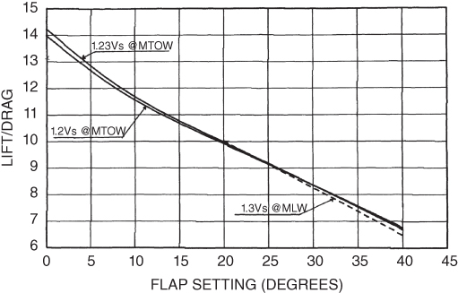
Figure 11.14 Drag polar with single‐slotted Fowler flap extended (undercarriage retracted).
11.15.2 Dive Brakes and Spoiler Drag
To decrease aircraft speed, whether in combat action or at landing, flat plates – which are attached to the fuselage and shaped to its geometric contour when retracted – are used. They could be placed symmetrically on both sides of the wing or on the upper fuselage (i.e. for military aircraft). The flat plates are deployed during subsonic flight. Use CDπ_brake = 1.2–2.0 (average 1.6) based on the projected frontal area of the brake to air stream. The force level encountered is high and controlled by the level of deflection. The best position for the dive brake is where the aircraft moment change is the least (i.e. close to the aircraft CG line).
11.15.3 Undercarriage Drag
Undercarriages, fixed or extended (i.e. retractable type), cause considerable drag on smaller, low‐speed aircraft. A fixed undercarriage (not streamlined) can cause up to about a third of aircraft parasite drag. When the undercarriage is covered by a streamlined wheel fairing, the drag level can be halved. It is essential for high‐speed aircraft to retract the undercarriage as soon as it is safe to do so (like birds). Below a 200 ft altitude from takeoff and landing, an aircraft undercarriage is kept extended.
The drag of an undercarriage wheel is computed based on its frontal area: Aπ_wheel (product of wheel diameter and width). For twin side‐by‐side wheels, the gap between them is ignored and the wheel drag is increased by 50% from a single‐wheel drag. For the bogey type, the drag also would increase – it is assumed by 10% for each bogey, gradually decreasing to a total maximum 50% increase for a large bogey. Finally, interference effects (e.g. due to undercarriage doors and tubing) would double the total of wheel drag. The drag of struts is computed separately. The bare single‐wheel CD_wheel based on the frontal area is in Table 11.6 (wheel aspect ratio = D/Wb).
Table 11.6 Bare single‐wheel drag with side ridge.
| Wheel aspect ratio (diameter/width) | 3 | 4 | 5 | 6 |
| CDπ_wheel | 0.15 | 0.25 | 0.28 | 0.3 |
For the smooth side, reduce by half. In terms of an aircraft:
A circular strut has nearly twice the amount of drag compared to a streamlined strut in a fixed undercarriage. For example, the drag coefficient of a circular strut based on its cross‐sectional area per unit length is CDπ_strut = 1.0 as it operates at a low Re during takeoff and landing. For streamlined struts with fairings, it decreases to 0.5–0.6, depending on the type.
Toreenbeck [10] suggests using an empirical formula if details of undercarriage sizes are not known at an early conceptual design phase. This formula is given in the FPS system as follows:
Understandably, it could result in a slightly higher value (see the following example). If aircraft geometry is available then it is advisable to accept the computed drag values as worked out next.
Worked-Out Example Worked-Out Example
Continue with the previous example using the largest in the design (i.e. maximum takeoff mass (MTOM) = 24 200 lb. and SW = 323 ft2) for the undercarriage size. It has a twin‐wheel, single‐strut length of 2 ft. (i.e. diameter of 6 in., Aπ_strul ≈ 0.2 ft2) and a main wheel size of a 22 in. diameter and a 9.6 in. width (i.e. wheel aspect ratio = 3.33, Aπ_wheel ≈ 1 ft2). From 11.6, a typical value of CDπ_wheel = 0.18, based on the frontal area and increased by 50% for the twin wheel (i.e. CD0 = 0.27). Including the nose wheel (although it is smaller and a single wheel, it is better to be liberal in drag estimation), the total frontal area is about 3 ft2: (A more accurate approach will be to consider the nose and mail wheels separately.)
- fwheel = 0.27 × 3 = 0.81 ft2 (nose wheel included)
- fstrut = 1.0 × 3 × 2 × 0.2 = 1.2 ft2 (nose wheel included)
Total fUC = 2 × (0.81 + 1.2) = 4.02 ft2 (100% increase due to interference, doors, tubing, and so on) in terms of CDpmin_UC = 4.02/323 = 0.0124. Checking the empirical relation in Eq. 11.43, CD_UC = 0.00 403 × (24 2000.785)/323 = 0.034, this may be taken if undercarriage geometric details are not available.
11.15.4 One‐Engine Inoperative Drag
Mandatory requirements by certifying agencies (e.g. Federal Aviation Administration, FAA and Civil Aeronautics Agency, CAA) specify that multiengine commercial aircraft must be able to climb at a minimum specified gradient with one engine inoperative at a ‘dirty’ configuration. This immediately safeguards an aircraft in the rare event of an engine failure; and in certain cases, after lift‐off. Certifying agencies require backup for mission‐critical failures to provide safety regardless of the probability of an event occurring.
Asymmetric drag produced by the loss of an engine would make an aircraft yaw, requiring a rudder to fly straight by compensating for the yawing moment caused by the inoperative engine. Both the failed engine and rudder deflection substantially increase drag, expressed by CDengine out + rudder. Typical values for coursework are in Table 11.7.
Table 11.7 One‐engine inoperative drag.
| ΔCDone engine out + ruddert | |
| Fuselage‐mounted engines | 0.003 5 |
| Wing‐mounted twin engine | 0.004 5 |
| Wing‐mounted four engine (outboard failure) | 0.005 |
11.16 Propeller‐Driven Aircraft Drag
Drag estimation of propeller‐driven aircraft involves additional considerations. The slipstream of a tractor propeller blows over the nacelle, which blocks the resisting flow. Also, the faster flowing slipstream causes a higher level of skin friction over the downstream bodies. This is accounted for as a loss of thrust, thereby keeping the drag polar unchanged. The following two factors arrest the propeller effects with piston engines (see Chapter 12 for calculating propeller thrust):
- blockage factor, fb, for tractor‐type propeller: 0.96–0.98 applied to thrust (for the pusher type, there is no blockage; therefore, this factor is not required – i.e. fb = 1.0)
- a factor, fh, as an additional profile drag of a nacelle: 0.96–0.98 applied to thrust (this is the slipstream effect applicable to both types of propellers)
Turboprop nacelles have a slightly higher value of fb than piston‐engine types because of a more streamlined shape. For the worked‐out example take fb × fh = 0.98 as an optimistic design. Typically, it is about 0.96.
11.17 Military Aircraft Drag
Military aircraft drag estimation requires additional considerations to account for the weapon system because most are external stores (e.g. missiles, bombs, drop tanks, flares and chaff launchers); few are carried inside the aircraft mouldlines (e.g. guns, ammunition and bombs inside the fuselage bomb bay, if any). Without external carriages, military aircraft are considered at typical configuration (the pylons are not removed – part of a typical configuration). Internal guns without their consumables are considered a typical configuration; with armaments, the aircraft is considered to be in a loaded configuration. In addition, most combat aircraft have a supersonic speed capability, which requires additional supersonic‐wave drag.
Rather than drag being due to passenger doors and windows as in a civil aircraft, military aircraft have additional excrescence drag (e.g. gun ports, extra blisters and antennas and pylons) that requires a drag increment. To account for these additional excrescences [3], suggests an increment of the clean flat plate equivalent drag, f, by 28.4%.
Streamlined external store drag is shown in Table 11.8 based on the frontal maximum cross‐sectional area. Bombs and missiles flush with the aircraft contour line have minor interference drag and may be ignored at this stage. Pylons and bomb racks create interference, and Eq. 11.24 is used to estimate interference on both sides (i.e. the aircraft and the store). These values are highly simplified at the expense of unspecified inaccuracy; readers should be aware that these simplified values are not far from reality (see [1, 4, 5] for more details).
Table 11.8 External store drag.
| External store | CDπ (based on frontal area) |
| Drop tanks | 0.1–0.2 |
| Bombs (length/diameter < 6) | 0.1–0.25 |
| Bombs/missiles (length/diameter > 6) | 0.25–0.35 |
Military aircraft engines are generally buried into the fuselage and do not have nacelles and associated pylons. Intake represents the air‐inhalation duct. Skin friction drag and other associated 3D effects are integral to fuselage drag, but their intakes must accommodate large variations of intake air‐mass flow. Military aircraft intakes operate supersonically; their power plants are low bypass turbofans (i.e. on the order of less than 3.0 – earlier designs did not have any bypass). For speed capabilities higher than Mach 1.9, most intakes and exhaust nozzles have an adjustable mechanism to match the flow demand in order to extract the best results. In general, the adjustment aims to keep the Vintake/V∞ ratio more than 0.8 over operational flight conditions, thereby practically eliminating spillage drag (see Figure 11.8). Supersonic flight is associated with shock‐wave drag.
11.18 Supersonic Drag
A well substantiated reference for industrial use is [3], which was prepared by Lockheed as a NASA contract for the National Information Service, published in 1971. A comprehensive method for estimating supersonic drag that is suitable for classroom work is derived from this exercise. The empirical methodology (called the Delta Method) is based on regression analyses of 18 subsonic and supersonic military aircraft (i.e. the T‐2B, T37B, KA‐3B, A‐4F, TA‐4F, RA‐5C, A‐6A, A‐7A, F4E, F5A, F8C, F‐11F, F100, F101, F104G, F105B, F106A and XB70) and 15 advanced (i.e. supercritical) aerofoils. The empirical approach includes the effects of the following:
- wing geometry (AR, t/c and aerofoil section)
- cross‐sectional area distribution
- CD variation with CL and Mach number
The methodology presented herein follows [3], modified to simplify CDp estimation resulting in minor discrepancies. The method is limited and may not be suitable to analyse more exotic aircraft configurations. However, this method is a learning tool for understanding the parameters that affect supersonic aircraft drag build‐up. Results can be improved when more information is available.
The introduction to this chapter highlights that aircraft with supersonic capabilities require estimation of CDpmin at three speeds: (i) at a speed before the onset of wave drag; (ii) at Mcrit and (iii) at maximum speed. The first two speeds follow the same procedure as for the high‐subsonic aircraft discussed in Sections 11.7 through 11.15. In the subsonic drag estimation method, the viscous‐dependent CDp varying with the CL is separated from the wave drag, CDw (i.e. transonic effects), which also varies with the CL but is independent of viscosity.
For book‐keeping purposes in supersonic flight, such a division between the CDp and the CDw is not clear with the CL variation. In supersonic speed, there is little complex transonic flow over the body, even when the CL is varied. It is not clear how shock waves affect the induced drag with a change in the angle of attack. For simplicity, however, in the empirical approach presented here, it is assumed that supersonic drag estimation can use the same approach as the subsonic‐drag estimation by keeping CDp and CDw separate. The CDp values for the worked‐out example are listed in Table 11.24. Here, drag due to shock waves is computed at CL = 0, and CDw is the additional shock‐wave drag due to compressibility varying with CL > 0. The total supersonic‐aircraft drag coefficient can then be expressed as follows:
It is recommended that in current practice, CFD analysis should be used to obtain the variation of CDp and CDw with CL. Reference [3] was published in 1978 using aircraft data before the advent of CFD. Readers are referred to [1, 4, 5] for other methods. The industry has advanced methodologies, which are naturally more involved.
The aircraft cross‐section area distribution should be as smooth as possible, as discussed in Section 5.10.2 (see Figure 5.15). It may not always be possible to use narrowing of the fuselage when appropriate distribution of areas may be carried out.
The stepwise empirical approach to estimate supersonic drag is as follows. The procedure is worked out in detail in Section 11.22.7.
- Step 1. Progress in the same manner as for subsonic aircraft to obtain the aircraft‐component Re for the cruise flight condition and the incompressible CFcomponent.
- Step 2. Increase CFcomponent in Step 1 by 28.4% as the military aircraft excrescence effect.
- Step 3. Compute CDpmin at the three speeds discussed previously.
- Step 4. Compute induced drag using CDi = C2/πAR.
- Step 5. Obtain CDp from the CFD and tests or from empirical relations.
- Step 6. Plot the fuselage cross‐section area versus the length and obtain the maximum area, Sπ, and base area, Sb (see e.g. Figure 11.21).
- Step 7. Compute the supersonic‐wave drag at zero lift for the fuselage and the empennage using graphs; use the parameters obtained in Step 6.
- Step 8. Obtain the design CL and the design Mach number using graphs (see Figures 11.27 and 11.28).
- Step 9. Obtain the wave drag, CDw, for the wing using the graphs.
- Step 10. Obtain the wing‐fuselage interference drag at supersonic flight using graphs.
- Step 11. Total all the drag values to obtain the total aircraft drag and plot as CD versus CL.
The worked‐out example for the North American RA‐5C Vigilante aircraft is a worthwhile coursework exercise. Details of the Vigilante aircraft drag are in [3]. The subsonic drag estimation methodology described in this book differs with what is presented in [3], yet is in agreement with it. The supersonic drag estimation follows the methodology described in [3]. A typical combat aircraft of today is not too different than the Vigilante in configuration details and similar logic can be applied. Exotic shapes (e.g. the F117 Nighthawk) should depend more on information generated from CFD and tests along with the empirical relations. For this reason, the author does not recommend undertaking coursework on exotic aircraft configurations unless the results can be substantiated. Learning with a familiar design that can be substantiated gives confidence to practitioners. Those in the industry are fortunate to have access to more accurate in‐house data.
11.19 Coursework Example – Civil Bizjet Aircraft
Figure 11.15a gives a three‐view diagram of the Bizjet as the coursework example. Its dissected aircraft components are given in Figure 11.15b.
Figure 11.15 Bizjet aircraft‐component diagram. (a) A three‐view diagram of the Bizjet. (b) Dissected aircraft components, isolated.
11.19.1 Geometric and Performance Data
The geometric and performance parameters discussed herein were used in previous chapters. Figure 11.15 illustrates the dissected anatomy of the coursework baseline aircraft.
Aircraft cruise performance for the basic drag polar is computed as follows:
Cruise altitude = 40 000 ft., LRC Mach = 0.65 (630 ft s−1) to 0.7 (678.5 ft s−1) at high altitudes. The Bizjet CDpmin is evaluated at 0.7 Mach as Bizjets cruises at high altitudes. The 2D flat plate CF_basic decreases as Re increases.
| Ambient pressure = 391.68 lb ft−2 | Ambient temperature = 390 K |
| Ambient density = 0.00 058 sl ft−3 | Ambient viscosity = 2.9 690 9847 × 10−7 lb. s ft−2 |
Re/ft. = 1.325 × 10⁶ (use incompressible zero Mach line as explained in Section 11.8.1).
CL at LRC (Mach 0.7) ≈ 0.5, CL at HSC (Mach 0.75) ≈ 0.4
| Fuselage | |||||
| Fuselage length, Lf = 15.24 m (50 ft) | Average diameter = 175.5 cm (70 in.) | ||||
| Overall width = 175 cm (69 in.) | Overall height (depth) = 178 cm (70 in.) | ||||
| Average diameter at the constant cross‐section barrel | Df = 1.765 m (5.74 ft). | ||||
| Fuselage upsweep angle 10° | Fuselage closure angle 10° | ||||
| Fineness ratio = Lf /Df = 8.633 | |||||
| Wing | |||||
| Aerofoil: NACA 65‐410 having 10% thickness to chord ratio for design CL = 0.4 | |||||
| Planform reference area | SW = 30 m2 (323 ft2) | Span = 15 m (49.2 ft), | AR = 7.5 | ||
| Wing MAC = 2.132 m (7 ft) | Dihedral = 3° | Twist = 2° (wash out) | t/c = 10% | ||
| Root chord at centreline, CR = 2.87 m (9.4 ft) | Tip chord, CT = 1.143 m (3.75 ft) | ||||
| Taper ratio λ = 0.4, | Quarter‐chord wing sweep = 14° | ||||
| H‐tail (Tee tail, aerofoil 64‐210 – installed with negative camber) | |||||
| Planform (Reference) area SH = 5.88 m2 (63.3 ft2) | Span = 5.15 m (16.7 ft), AR = 4.22 | ||||
| Root chord, CR = 1.54 m (5.04 ft) | Tip chord CT = 0.77 m (2.52 ft) | ||||
| H‐tail MAC = 1.19 m (3.9 ft) | Taper ratio λ = 0.5, Λ¼ = 15° | ||||
| Dihedral = 5° | Elevator = 1.21 m2 (13 ft2), t/c = 10% | ||||
| V‐tail (aerofoil 64‐010) | |||||
| Planform (Reference) area SV = 4.4 m2 (47.3 ft2) | Height = 2.14 m (7 ft), AR = 2.08 | ||||
| Root chord, CR = 2.57 m (8.43 ft) | Tip chord, CT = 1.54 m (5.05 ft) | ||||
| V‐tail MAC = 2.07 (6.8 ft) | Taper ratio, λ = 0.6, Λ¼ = 40° | ||||
| Rudder = 0.75 m2 (8 ft2) | t/c = 10% | ||||
| Nacelle (each – two required) | |||||
| Length = 2.84 m (9.3 ft) | Maximum diameter = 1.074 m (3.52 ft) | ||||
| Nacelle fineness ratio = 2.62/1.074 = 2.44 | |||||
| Bare engine (each – two required) | |||||
| Honeywell TFE731‐20 turbofan | |||||
| Takeoff static thrust at International Standard Atmosphere (ISA) sea level = 3800 lb. (17 235 N) per engine with bypass ratio (BPR) = 4 | |||||
| Dry weight = 379 kg (836 lb) | Fan diameter = 0.716 m (28.2 in.) | Length = 1.547 m (60.9 in.) | |||
11.19.2 Computation of Wetted Areas, Re and Basic CF
The aircraft is dissected in to isolated components as shown in Figure 11.15. The Re, wetted area, and basic 2D flat plate CF_basic of each component are worked‐out herein. Bizjet CDpmin is evaluated at 0.7 Mach.
| Fuselage | |
| The fuselage is conveniently sectioned into three parts: | |
| 1. Front fuselage length, LFf = 3.5 m with a uniformly varying cross‐section | |
| 2. Mid‐fuselage length LFm = 5.95 m with an average constant cross‐section diameter = 1.765 m | |
| 3. Aft‐fuselage length LFa = 5.79 m, with a uniformly varying cross‐section | |
| Wetted area | |
| Front fuselage, AwFf (no cutout) = 110 ft2 | |
| Mid‐fuselage, AwFm (with two sides of wing cut‐outs) = 352 − 2 × 6 = 340 ft2 | |
| Aft fuselage, AwFs (with empennage cut‐outs) = 180 − 10 = 170 ft2 | |
| Include additional wetted area for the wing‐body fairing housing the undercarriage ≈ 50 ft2 | |
| Total wetted area, Awf = 110 + 340 + 170 + 50 = 670 ft2 | |
| Fuselage Re = 50 × 1.325 × 106 = 6.625 × 10⁷ | |
| Fineness ratio = Lf /Df = 8.633 | |
| From Figure 11.24, bottom graph (fully turbulent) at LRC, the incompressible basic CFf = 0.0022. | |
| Wing | |
| Wing exposed reference area = 323 − 50 (area buried in the fuselage) = 273 ft2 | |
| MAC = 2.132 m (7 ft), AR = 7.5 | |
| For t/c = 10% of the wing wetted area, Aww = 2.024 × 273 = 552.3 ft2 (see Section 11.8.2.1) | |
| Root chord, CR = 2.87 m (9.4 ft) | |
| Tip chord, CT = 1.143 m (3.75 ft) | |
| Wing Re = 7 × 1.325 × 106 = 9.275 × 10⁶ | |
| From Figure 11.24, bottom graph at LRC, the incompressible basic CFw = 0.003 | |
| Empennage (same procedure as for the wing) | |
| H‐tail | |
| Planform (Reference) area SH = 5.88 m2 (63.3 ft2) | AR = 4.22 |
| H‐tail MAC = 1.19 m (3.9 ft) | Taper ratio, λ = 0.5 |
| It is a T‐tail and it is fully exposed. | |
| for t/c = 10%, the H‐tail wetted area, AwHT = 2.024 × 63.3 = 128.12 ft2 | |
| H‐tail Re = 3.9 × 1.325 × 106 = 5.17 × 10⁶ | |
| From Figure 11.24, bottom graph (fully turbulent) at LRC, the incompressible basic CF_H−tail = 0.0032 | |
| V‐tail | |
| Planform (Reference) area, SV = 4.4 m2 (47.3 ft2) | AR = 2.08 |
| Root chord, CR = 2.57 m (8.43 ft) | Taper ratio, λ = 0.6 Λ¼ = 40° |
| Empennage (same procedure as for the wing) | |
| Exposed reference area = 47.3 − 7.3 (approximate area buried in the fuselage) = 40 ft2 | |
| For t/c = 10% the V‐tail wetted area, Aw_VT = 2.024 × 40 = 81 ft2 | |
| MAC = 2.07 m (6.8 ft) | |
| V‐tail Re = 6.8 × 1.325 × 106 = 9.01 × 10⁶ | |
| From Figure 11.24, bottom graph (fully turbulent) at LRC, the incompressible basic CF_V−tail = 0.003 | |
| Nacelle | |
| Length = 2.84 m (9.3 ft) | maximum diameter = 1.074 m (3.52 ft) |
| Average diameter ≈ 0.8 m (2.62 ft) | fineness ratio = 3.55 |
| Nacelle Re = 9.3 × 1.325 × 106 = 1.23 × 10⁷ | |
| Two‐nacelle wetted area, Awn = (2 × 3.14 × 3.55 × 9.3) − 2 × 5 (two pylon cut‐outs) = 197.3 ft2 | |
| From Figure 11.24, bottom graph (fully turbulent) at LRC, the incompressible basic CF_nac = 0.0029 | |
| Pylon | |
| Each pylon exposed reference area = 14 ft2 | |
| Length = 2.28 m (7.5 ft), t/c = 10% | |
| Two pylon wetted area Awp = 2 × 2.024 × 14 = 56.7 ft2 | |
| Pylon Re = 7.5 × 1.325 × 106 = 9.94 × 10⁶ | |
| From Figure 11.24, bottom graph (fully turbulent) at LRC the incompressible basic CFpylon = 0.00 295. | |
Table 11.9 summarises the Bizjet component Re and 2D basic skin friction CFbasic.
Table 11.9 Summary of Bizjet component Reynolds Number and 2D basic skin friction CFbasic.
| Parameter | Reference area (ft2) | Wetted area (ft2) | Characteristic length (ft) | Reynolds Number | 2D CF_basic |
| Fuselage | n/a | 670 | 50 | 6.625 × 10⁷ | 0.002 2 |
| Wing | 323 | 552.3 | 7 (MACw) | 9.275 × 10⁶ | 0.003 |
| V‐Tail | 4.4 | 81 | 6.8 (MACVT) | 9.01 × 10⁶ | 0.003 |
| H‐Tail | 65.3 | 128.12 | 3.9 (MACHT) | 5.17 × 10⁶ | 0.003 2 |
| 2 × Nacelle | n/a | 197.3 | 9.3 | 1.23 × 10⁷ | 0.002 9 |
| 2 × Pylon | 2 × 14 | 56.7 | 7.5 | 9.94 × 10⁶ | 0.00 295 |
11.19.3 Computation of 3D and Other Effects to Estimate Component CDpmin
A component‐by‐component example of estimating CDpmin is provided in this section. The corrected CF for each component at LRC (i.e. Mach 0.7) is computed in the previous section.
- Fuselage
The basic CFf = 0.0022
3D effects (Eqs. 11.16–11.18).
Wrapping: ΔCFf = CFf × 0.025 × (length/diameter) × Re−0.2
- = [0.0022 × 0.025 × (8.633)] × (6.625 × 10⁷)−0.2
- = 0.000 475 × 0.0273 = 0.000 013 (5.9% of basic CFf)
Supervelocity: ΔCFf = CFf × (diameter/length)1.5 = 0.0022 × (1/8.633)1.5
- = 0.0022 × (0.1158)1.5 = 0.0 000 867 (3.94% of basic CFf)
Pressure: ΔCFf = CFf × 7 × (diameter/length)3 = 0.0022 × 7 × (0.1158)3
- = 0.0154 × 0.001 553 = 0.0 000 239 (1.09% of basic CFf)
| Other effects on fuselage (see Section 11.9.1) | |
| Body pressurisation – fuselage surface waviness: | 4% |
| Non‐optimum fuselage shape | |
| (a) nose fineness – for 1.5 ≤ Fcf ≤ 1.75: | 6% |
| (b) fuselage closure – less than 10°: | 0 |
| (c) upsweep closure – 10° upsweep: | 6% |
| (d) aft‐end cross‐sectional shape – circular: | 0% |
| Cabin‐pressurisation leakage (if unknown, use higher value): | 4% |
| Excrescence (non‐manufacturing types, e.g. windows) | |
| (a) windows and doors: | 2% |
| (b) miscellaneous: | 1% |
| Wing‐fuselage‐belly fairing, if any (higher value if it houses undercarriage): | 1% |
| ECS (see Section 11.8) gives 0.06 ft2 | 2.8% |
| Total other effects ΔCFf_other effects increment: | 26.8% |
Table 11.10 gives the Bizjet fuselage CFf components.
Table 11.10 Bizjet fuselage ΔCFf correction (3D and other shape effects).
| Item | ΔCFf | % of CFfbasic |
| Wrapping | 0.000 013 | 6.9 |
| Supervelocity | 0.0 000 867 | 3.94 |
| Pressure | 0.0 000 239 | 1.09 |
| Body pressurisation | 5 | |
| Fuselage upsweep of 10° | 6 | |
| Fuselage closure angle of 9° | 0 | 0 |
| Nose fineness ratio 1.7 | 4 | |
| Aft‐end cross‐section – circular | ||
| Cabin‐pressurisation/leakage | 4 | |
| Excrescence (windows/doors etc.) | 2 | |
| Belly fairing | 1 | |
| Environ. Control System Exhaust (ECS) | 2.8 | |
| Total ΔCFf | 0.0 001 236 | 33.93 ≈ 34 |
Add the canopy drag for two‐abreast seating f = 0.1 ft2 (see Section 11.9.1).
Therefore, the equivalent flat plate area, f, becomes = CFf × AwF + canopy drag.
ff = 1.34 × 0.0022 × 670 + 0.1 = 1.975 + 0.1 = 2.075 ft2
Surface roughness (to be added later): 3%
- Wing
Basic CFW = 0.003
3D effects (Eqs. 11.15–11.17):
Supervelocity: ΔCFw = CFw × 1.4 × (aerofoil thickness/chord ratio)
- = 0.003 × 1.4 × 0.1 = 0.00 042 (14% of basic CFw)
Pressure: ΔCFw = CFw × 60 × (aerofoil thickness/chord ratio)4 × ![]()
- = (0.003 × 60) × (0.1)4 × (6/7.5)0.125
- = 0.18 × 0.0001 × 0.9725 = 0.0 000 175 (0.58% of basic CFw)
Interference: ΔCFw = CB2× 0.6 × ![]()
- = 92 × 0.6 × [{0.75 × (0.1)3 − 0.0003}/552.3]
- = 81 × 0.6 × (0.00 075 − 0.0003)/552.3
- = 0.0219/552.3 = 0.00 004 (1.32% of basic CFw)
Other effects:
Excrescence (non‐manufacturing, e.g. control surface gaps etc.):
| Flap gaps | 5% |
| Others | 5% |
| Total ΔCFw increment = | 25% |
Table 11.11 summarises Bizjet wing ΔCFw correction (3D and other shape effects).
Table 11.11 Bizjet wing ΔCFw correction (3D and other shape effects).
| Item | ΔCFw | % of CFwbasic |
| Supervelocity | 0.00 042 | 14 |
| Pressure | 0.0 000 175 | 0.58 |
| Interference (wing‐body) | 0.00 004 | 1.32 |
| Flaps gap | 5 | |
| Excrescence (others) | 5 | |
| Total ΔCFw | 26 |
Therefore, in terms of equivalent flat plate area, f, it becomes = CFw × Aww
Surface roughness (to be added later) 3%.
- Empennage
Since it follows the same procedure as in the case of wing, this is not repeated. The same percentage increment as the case of wing is taken as a classroom exercise. It may be emphasised here that in industry, one must compute systematically as shown in the case of the wing.
| H‐tail: | Wetted area, AwHT = 128.12 ft2 | Basic CF_V‐tail = 0.0032 |
| fHT = 1.26 × 0.0032 × 128.12 = 0.5166 ft2 | ||
| Surface roughness (to be added later) | 3% | |
| V‐tail: | Wetted area, AwVT = 81 ft2, | Basic CF_H‐tail = 0.003 |
| It is T‐tail configuration having interference from T‐tail (add another 1.2%). | ||
| fVT = 1.26 × 0.003 × 81 = 0.306 ft2 | ||
- Nacelle
Fineness ratio = 2.44, Nacelle Re = 1.23 × 10⁷.
Wetted area of two nacelles, Awn = 197.3 ft2, Basic CFnac = 0.0029
3D effects (Eqs. 11.15–11.17):
Wrapping (Eq. 11.10): ΔCFn = CFn × 0.025 × (length/diameter) × Re−0.2
- = (0.025 × 0.003 × 2.44) × (1.23 × 107)−0.2
- = 0.000 183 × 0.0382 = 0.000 007 (0.24% of basic CFf)
Other increments are shown in Table 11.12 for one nacelle.
Table 11.12 Bizjet nacelle ΔCFn correction (3D and other shape effects).
| Item (one nacelle) | ΔCFn | % of CFnbasic |
| Wrapping (3D effect) | 0.000 007 | 0.24 |
| Excrescence (non‐manufacture) | 22 | |
| Boat Tail (aft end) | 10 | |
| Base drag (at cruise) | 0 | 0 |
| Intake drag (BPR 4) | 40 | |
| Total ΔCFn | 72.24 |
| For two nacelles (shown in wetted area) | fn = 1.7224 × 0.0029 × 197.3 = 0.986 ft2 |
| Surface roughness (to be added later) | 3% |
- Pylon
Since it follows the same procedure as in the case of wing, this is not repeated. The same percentage increment as the case of wing is taken as a classroom exercise. It has interference at both sides of pylon.
Each pylon exposed reference area = 14 ft2.
| Length = 2.28 m (7.5 ft), t/c = 10%, | Two pylon wetted area Awp = 56.7 ft2 |
| 7.5 × 1.325 × 106 = 9.94 × 10⁶, | Basic CFpylon = 0.00 295 |
| For two pylons (shown in wetted area) | fpy = 1.26 × 0.00 295 × 56.7 = 0.21 ft2 |
| Surface roughness (to be added later) | 3% |
11.19.4 Summary of Parasite Drag
Table 11.13 gives the aircraft parasite drag build‐up summary in a tabular form. Surface roughness effect as 3% increase (Eq. 11.28) in ‘f’ is added in this table for all surfaces. Wing reference area Sw = 323 ft2, CDpmin = f/Sw. ISA day, 40 000 ft. altitude and Mach 0.7.
Table 11.13 Bizjet parasite drag build‐up summary and CDpmin estimation.
| Wetted area, Aw ft2 | Basic CF | ΔCF | Total CF | f (ft2) | CDpmin | |
| Fuselage + U/C fairing | 670 | 0.002 2 | 0.000 748 | 0.002 948 | 1.975 | 0.00 611 |
| Canopy | 0.1 | 0.00 031 | ||||
| Wing | 552.3 | 0.003 | 0.00 078 | 0.003 784 | 2.09 | 0.00 647 |
| V‐tail | 81 | 0.003 | 0.000 786 | 0.003 786 | 0.302 | 0.00 095 |
| H‐tail | 128.12 | 0.003 2 | 0.000 936 | 0.00 414 | 0.53 | 0.00 164 |
| 2 × Nacelle | 2 × 79 | 0.002 9 | 0.002 386 | 0.00 528 | 0.986 | 0.00 305 |
| 2 × Pylon | 2 × 28 | 0.00 295 | 0.000 767 | 0.00 372 | 0.21 | 0.00 065 |
| Rough (3%) | Eq. 11.28 | 0.186 | 0.00 057 | |||
| Air‐condition | 0.06 | 0.000 186 | ||||
| Aerial, lights | 0.03 | 0.000 093 | ||||
| Trim drag | 0.13 | 0.000 4 | ||||
| Total |
6.599 ≈ 6.6 |
0.02 043 ≈ 0.020 5 |
||||
11.19.5 ΔCDp Estimation
Use Figure 11.16 for typical data (requires CFD/testing). The ΔCDp values used in the Bizjet are given in Table 11.14.

Figure 11.16 Drag polar of Figure 11.2 plotted CL2 versus CD.
Table 11.14 Bizjet ΔCDp estimation.
| CL | 0.1 | 0.2 | 0.3 | 0.4 | 0.5 | 0.6 | 0.7 |
| ΔCDp | 0.000 7 | 0.000 3 | 0.00 006 | 0 | 0.000 6 | 0.002 | 0.004 |
11.19.6 Induced Drag
Formula used CDi = CL2/(3.14 × 11.5) = CL2/23.55. The ΔCDi values used in Bizjet are given in Table 11.15.
Table 11.15 Bizjet induced drag.
| CL | 0.2 | 0.3 | 0.4 | 0.5 | 0.6 | 0.7 | 0.8 |
| CDi | 0.001 7 | 0.00 382 | 0.006 8 | 0.010 6 | 0.015 3 | 0.020 6 | 0.027 2 |
11.19.7 Total Aircraft Drag at LRC
Drag polar at LRC can be summed up as shown in Table 11.16.
Table 11.16 Bizjet total aircraft drag coefficient, CD.
| CL | 0.2 | 0.3 | 0.4 | 0.5 | 0.6 | 0.7 |
| CDpmin | 0.020 5 from Table 11.13 | |||||
| ΔCDp (Table 11.14) | 0.000 3 | 0.00 006 | 0 | 0.000 6 | 0.002 | 0.003 |
| CDi (Table 11.15) | 0.001 7 | 0.00 382 | 0.006 8 | 0.010 6 | 0.015 3 | 0.020 6 |
| Total aircraft CD @ LRC | 0.022 5 | 0.02 438 | 0.027 3 | 0.031 7 | 0.037 8 | 0.044 1 |
| Wave drag, CDw (Figure 11.10b) | 0.001 4 | 0.001 7 | 0.002 | 0.002 5 | 0.003 2 | 0.004 5 |
| Total aircraft CD @ HSC | 0.023 9 | 0.02 608 | 0.029 3 | 0.034 2 | 0.041 | 0.048 6 |
Drag polar at HSC (Mach 0.75) would require adding wave drag.
This drag polar is plotted in Figure 11.2. CL2 versus CD is plotted in Figure 11.16. Note the non‐linearity at low and high CL..
11.20 Classroom Example – Subsonic Military Aircraft (Advanced Jet Trainer – AJT)
The classroom example of military aircraft example was conducted on a subsonic AJT/Close Air Support (CAS) type of aircraft of the class BAE Hawk that would follow the same procedure as the civil aircraft drag estimation method. To avoid repetition, only the drag polar and other drag details of the AJT are given in Figure 11.17.

Figure 11.17 AJT drag polar (Section 11.20).
Figure 11.18 gives the three‐view diagram of the AJT (of the class of BAE Hawk trainer) and its variant CAS aircraft. Given next is the defence specification for which the design has developed. HSC Mach = 0.85 at a 9 km altitude, LRC Mach = 0.78 at a 9 km altitude

Figure 11.18 AJT and its CAS variant.
The important external dimensions of the baseline AJT design are as follows.
| Fuselage (Baseline) | |
| Length = 12 m (39.4 ft) | |
| Maximum overall width = 1.8 m (5.9 ft) | Overall height (depth) = 4.2 m (13.78 ft) |
| Cockpit width = 0.88 m (2.89 ft) | Fineness ratio = 12/1.8 = 6.67 |
| Wing | |
| Planform (reference) area = 17 m2 (183 ft2) | Span = 9.5 m (31.17 ft), AR = 5.31 |
| Root chord, CR = 2.65 m (8.69 ft) | Tip chord, CT = 0.927 m (3.04 ft) |
| MAC = 1.928 (6.325 ft) | Taper ratio, λ = 0.35, Λ¼ = 20° |
| Dihedral = −2°. (anhedral – high wing) | Twist = 1° (wash out) |
| Flap = 2.77 m2 (29.8 ft2) | Aileron = 1.06 m2 (11.4 ft2) |
| H‐tail | |
| Planform (Reference) area = 4.7 m2 (50.32 ft2) | Span = 4.2 m (13.8 ft) |
| Root chord, CR = 1.9 m (6.23 ft) | Tip chord, CT = 0.57 m (1.87 ft) |
| MAC = 1.354 m (4.44 ft) | Taper ratio, λ = 0.3, Λ¼ = 25° |
| AR = 3.5 | Tail arm = 4 m (13.1 ft) |
| Elevator area = 0.956 m2 (10.3 ft2) | t/c = 10% |
| V‐tail | |
| Planform (Reference) area = 3.83 m2 (41.1ft2) | Span = 2.135 m (7 ft) |
| Root chord, CR = 2.2 m (7.22 ft) | Tip chord CT = 0.57 m (1.87 ft) |
| MAC = 1.545 m (5 ft) | Taper ratio λ = 0.26, Λ¼ = 35° |
| AR = 1.52 | Tail arm = 4 m (13.1 ft) |
| Rudder area = 0.98 m2 (10.5ft2) | t/c = 9% |
| Nacelle: | None as the engine is buried into the fuselage. |
| Engine | |
| Takeoff static thrust at ISA sea level = 5390 lb. | BPR = 0.75 |
| Fan diameter = 0.56 m (22 in.) | Length = 1.956 m (77 in.) |
| Maximum depth = 1.04 m (3.4 ft) | Maximum width = 0.75 m (2.46 ft) |
| Baseline aircraft mass (from statistics – needs to generated from the variant CAS design.) | |
| MTOM = 6500 kg (15 210 lb) | NTCM = 4800 kg (10 800 lb) |
| Operator's empty mass (OEM) = 3700 kg | Fuel mass = 1100 kg (maximum capacity 1300 kg) |
CAS Variant (all component dimensions except fuselage length are kept unchanged).
The CAS role aircraft is the only variant of the AJT aircraft. Configuration of the CAS aircraft variant is achieved by splitting the AJT front fuselage, then replacing the tandem seat arrangement with a single seat cockpit. The length could be kept the same as the nose cone needs to house more powerful acquisition radar. The front loading of radar and single pilot is placed in a way that the CG location is kept undisturbed. Wing area = 17 m2 (183 ft2).
| Specifications | |
| Payload = 2500 kg | Range = |
| Mcrit = 0.85 Mach | MCR = 0.78 |
| Fuselage | |
| Length = 11.2 m (36.8 ft) | |
| Maximum overall width = 1.8 m | Overall height (depth) = 4.2 m |
| Cockpit width = 0.88 m | Fineness ratio = 11.2/1.8 = 6.22 |
Weights
The summary of mass changes is as follows. CAS mass has been derived by removing one pilot, the instrument ejection seat and so on (260 kg) and includes radar and combat avionics (100 kg). There is an increase of 60 kg in engine mass. Internal:
| AJT (kg) | CAS (kg) | |
| OEM | 3700 | 3700 |
| Fuel | 1100 | 1300 (full tank) |
| Clean aircraft MTOM | 4800 (10 582 lb) | 5000 (11 023 lb) |
| Wing loading*, W/SW | 282 kg m−2 (57.8 lb ft−2) | 294 kg m−2 (60.23 lb ft−2) |
| Armament mass | 1800 | 2200 |
| MTOM kg (lb) | 6500 (14 326 lb) | 7500 (16 535 lb) |
| Wing loading, W/SW | 382.2 kg m−2 (78.3 lb ft−2) | 441.2 kg m−2 (90.36 lb ft−2) |
Armament and fuel could be traded for range. Drop tanks could be used for ferry range.
The drag level of the clean AJT and CAS aircraft may be considered to be about the same. There would be an increase of drag on account of the weapon load. For the CAS aircraft, there is a wide variety, but to give a general perception, the typical drag coefficient increment for armament load is CDπ = 0.25 (includes interference effect) each for five hard points as weapon carrier. Weapon drag is based on maximum cross‐section (say 0.8ft2) area of the weapons.
Parasite drag increment due to armament, ΔCDpmin = (5 × 0.25 × 0.8)/183 = 0.0055, where SW = 183 ft2.
11.20.1 AJT Details
Drag polar at Mach 0.78 and at Mach 0.85 is tabulated in Table 11.17 and plotted in Figure 11.17. From this, AJT parabolic drag can approximated as CD = 0.0212 + 0.07 CL2 with SW = 183 ft2 (gives Oswald's efficiency factor, e = 0.85).
Table 11.17 AJT total aircraft drag coefficient, CD.
| CL | 0.1 | 0.2 | 0.3 | 0.4 | 0.5 | 0.6 |
| CDpmin | 0.021 2 (readers make work out) | |||||
| ΔCDp | 0.000 1 | 0.000 3 | 0.000 6 | 0.001 | 0.001 4 | 0.002 6 |
| CDi = CL2/(3.14 × 5.3) | 0.000 6 | 0.002 4 | 0.005 4 | 0.00 961 | 0.015 | 0.021 6 |
| Total aircraft CD @ 0.78 M | 0.021 9 | 0.023 9 | 0.027 2 | 0.03 181 | 0.037 6 | 0.045 4 |
| Wave drag, CDw | 0.001 6 | 0.001 8 | 0.002 | 0.00 271 | 0.003 3 | 0.005 6 |
| Total aircraft CD @ 0.85 M | 0.023 5 | 0.025 7 | 0.029 2 | 0.03 452 | 0.040 9 | 0.051 |
11.21 Classroom Example – Turboprop Trainer (TPT)
This an example of the drag estimation for a propeller‐driven aircraft. A classroom example of the TPT type aircraft of the class Shorts Tucano uses the same procedure as the civil aircraft drag estimation method. However, propeller‐driven aircraft drag has to account for the propeller slipstream effects on the wetted surface. Propeller wake has a higher velocity than the aircraft free‐stream velocity. This gives a different average skin friction coefficient, CF. There are also nacelle blockage factors that have to be considered. V‐Tail is given 1° offset to counter slipstream rotational effect.
To avoid repetition TPT drag evaluation is done in a short‐cut method (based on experience). Some of the flat plate equivalent drags ‘fs’ are given (using comparable industrial data). It is recommended that the readers should undergo the full methodology. The results should not be much different from the drag polar given here. The three‐view diagram of TPT is given in Figure 11.19, showing the slipstream effects. Normal Training Configuration (NTC) is an aircraft is without any weapon load; that is, no external stores.

Figure 11.19 Turboprop trainer aircraft (TPT).
Given next is the defence specification for which the design has developed. Practise altitude = 25 000 ft. (ρ = 0.00 106 slug ft−3 and μ = 0.3216 × 10⁻⁶ lbs ft−2). CDPmin = 0.023. The important TPT details are as follows.
| MTOM = 2800 kg (6170 lb) | NTC‐TOM = 2350 kg (5180 lb) |
| OEW = 4400 lb (2000 kg) | Typical mid‐training aircraft mass = 2200 kg (4850 lb) |
| Crew = 400 lb (≈180 kg) | Fuel = 1000 lb (≈450 kg) |
| Maximum speed = 280 kt | Sustained speed = 240 kt (405.2 ft s−1) |
| Fuselage | |
| Length = 30 ft | Overall height = 10 ft |
| Cockpit width = 35 in | Fineness ratio = (30 × 12)/35 = 10.3 |
| Wing (NACA 63‐212) | |
| Reference area = 16.5 m2 (177.3 ft2) | Span = 10.36 m (34 ft), AR = 6.5 |
| Root chord, CR = 2.36 m (7.74 ft) | Tip chord, CT = 0.82 m (2.7 ft) |
| MAC = 1.715 m (5.63 ft) | Taper ratio, λ = 0.35, Λ¼ = degrees |
| Dihedral = 5° (dihedral – low wing) | Twist = 1° (wash out), t/c = 0.12 |
| Flap = 2.77 m2 (29.8 ft2) | Aileron = 1.06 m2 (11.4 ft2) |
| H‐tail (NACA 0012) | |
| Reference area = 4.1 m2 (44.2 ft2) | Span = 4.16 m (13.8 ft), AR = 4.0 |
| Root chord, CR = 1.32 m (4.33 ft) | Tip chord, CT = 0.66 m (2.17 ft) |
| H‐tail MAC = 1.0234 m (3.36 ft) | Taper ratio, λ = 0.5, Λ¼ = 25° |
| Elevator area = 0.956 m2 (12 ft2) | t/c = 0.12 |
| V‐tail (NACA 0012) | |
| Reference area = 2.2 m2 (23.3 ft2) | Span = 1.615 m (5.3 ft), AR = 1.52 |
| Root chord, CR = 1.64 m (5.38 ft) | Tip chord, CT = 0.66 m (2.17 ft) |
| V‐tail MAC = 1.22 (4.0 ft) | Taper ratio, λ = 0.4, Λ¼ = 35° |
| Rudder area = 0.98 m2 (8 ft2) | t/c = 0.12 |
| Nacelle: | None as the engine is buried into the fuselage. |
11.21.1 TPT Details
ISA day, 25 000 ft. altitude. Wing reference area Sw = 16.5 m2 (177.38 m2). CDpmin = f/Sw. Cruise CL = 0.3.
Outstream velocity = 405.2 ft s−1 (≈ Mach 0.4)
Intstream velocity = 567.28 ft s−1 (increase 40%).
Outstream Re/ft. @ 25 000 ft at 405.2 ft s−1 = 1.3355 × 10⁶
Intstream Re/ft. @ 25 000 ft and at 567.28 ft s−1 = 1.87 × 10⁶
Drag estimation follows the Bizjet methodology incorporating slipstream effects. Note that a TPT does not have nacelles. Intake drag is to be estimated accordingly.
Quick component drag parasite drag estimation: The short‐cut method uses Bizjet ΔCF percentage increases. No credit is taken for partial laminar flow.
- Fuselage
The wetted surface of the fuselage is entirely in slipstream; in short, instream.
Fuselage instream Re is 5.6 × 10⁷ and corresponding basic CFf is 0.0022. Wetted area Awf = 280 ft2.
Unlike Bizjet, the TPT does not have (i) fuselage pressurisation, (ii) windows and doors, (iii) wing‐fuselage‐belly fairing and (iv) upsweep closure reducing ΔCFf by 20%. Take (i) wrapping, (ii) supervelocity and (iii) pressure together as 5%.
The basic CFf = 0.0022 (see Table 11.18).
Table 11.18 Summary of TPT component Reynolds Number and 2D basic skin friction CFbasic.
| Parameter | Reference area (ft2) | Wetted area (ft2) | Characteristic length (ft) | Reynolds Number | 2D CF_basic |
| Fuselage (instream) | n/a | 280 | 30 | 5.6 × 10⁷ | 0.002 2 |
| Wing (in) | 200 | 70 | 5.5 (MACw)a | 1.03 × 10⁷ | 0.002 9 |
| Wing (out) | 280 | 5.5 (kept same) a | 9.35 × 10⁶ | 0.003 | |
| V‐Tail (in) | 22 | 45 | 4.2 (MACVT) | 9.85 × 10⁶ | 0.00 298 |
| H‐Tail (in) | 20 | 40.6 | 3.3 (MACHT) a | 9.1 × 10⁶ | 0.00 304 |
| H‐Tail (out) | 24.2 | 50 | 3.3 (MACHT) a | 4.4 × 10⁶ | 0.003 5 |
| Strakes (in) |
V‐tail and strakes are instream.
aStrictly speaking, separate MAC should be taken. The error is small.
Take the 3D effects, for example, (i) wrapping, (ii) supervelocity and (iii) pressure together as 5% of the basic CFf.
Other effects on fuselage (see Section 11.9.1)
- (a) nose fineness – for 1.5 ≤ Fcf ≤ 1.75 : 6%
- (b) aft‐end cross‐sectional shape near circular: 0%
excrescence (non‐manufacturing types): 3%
- (c) miscellaneous: 1%
Total ΔCFf increment: ≈15%
Fuselage blockage factors of fb and fh are included as engine installation losses reducing thrust by about 3%. Therefore, fuselage blockage factors are not for accounted here.
Add the canopy drag for two‐abreast seating f = 0.1 ft2 (see Section 11.9.1).
Therefore, the equivalent flat plate area, f, becomes = CFf × AwF + canopy drag.
ffus = 1.15 × 0.0022 × 280 + 0.1 = 0.708 + 0.1 = 0.81 ft2.
Surface roughness (to be added later): 3%.
Table 11.19 summarises the TPT fuselage CFf.
- Wing:
Table 11.19 TPT parasite drag build‐up summary and CDpmin estimation.
| Wetted area, Aw ft2 | Basic CF | ΔCF | Total CF | f (ft2) | CDpmin | |
|
Fuselage + canopy |
280 | 0.002 2 | 0.00 035 | 0.00 266 | 0.81 | 0.004 |
| Wing in | 70 | 0.002 9 | 0.000 754 | 0.00 365 | 0.256 | 0.00 128 |
| Wing‐out | 280 | 0.003 | 0.00 078 | 0.00 378 | 1.06 | 0.005 3 |
| V‐tail | 45 | 0.00 298 | 0.000 775 | 0.00 376 | 0.17 | 0.00 085 |
| H‐tail‐in | 40.6 | 0.00 304 | 0.000 8 | 0.00 384 | 0.156 | 0.00 078 |
| H‐tail‐out | 50 | 0.003 5 | 0.00 091 | 0.00 441 | 0.22 | 0.001 1 |
| Strakes + dorsal | 0.05 | 0.00 025 | ||||
| Engine intake | 0.1 | 0.000 5 | ||||
| Exhaust stub | 0.2 | 0.001 | ||||
| NACA intakes | 0.8 | 0.004 | ||||
| Rough (3%) | 0.182 | 0.000 6 | ||||
| Excrescences | 0.106 | 0.00 053 | ||||
| Aerial, lights | 0.05 | 0.000 4 | ||||
| Trim drag | 0.13 | 0.00 001 | ||||
| Miscellaneous | 0.4 | 0.002 | ||||
| Total | 4.5 | 0.022 6 | ||||
Of the wing the wetted Awf surface, approximately 20% is instream and 80% is outstream.
Wetted area Aww = 320 ft2. Instream = Aww_in = 70 ft2 and outstream Aww_out = 250 ft2 and
Instream Rein = 1.03 × 10⁷ giving basic CFW_in = 0.0029 and outstream Reout = 1.135 × 10⁷ giving basic CFW_out = 0.003.
Take the 3D effects, for example, (i) interference, (ii) supervelocity and (iii) pressure together as 16% of the basic CFw. Other effects on wing:
Excrescence (non‐manufacturing, e.g. control surface gaps etc.):
| Flap gaps | 5% |
| Others | 5% |
| Total ΔCFw increment = | 26% |
- Empennage
Since it follows the same procedure as in the case of wing, this is not repeated. The same percentage increment as in the case of wing is taken as a classroom exercise. It may be emphasised here that in industry, one must compute systematically as shown in the case of the wing at 3% surface roughness (to be added later).
H‐tail: (of the H‐tail the wetted Awf surface, approximately 45% is instream and 55% is outstream).
Wetted area AwHT = 90.6 ft2. Instream = AwHT_in = 40.6 ft2 and outstream AwHT_out = 50 ft2
Instream Rein = 9.1 × 10⁶ giving basic CFW_in = 0.00 304
Outstream Reout = 4.4 × 10⁶ giving basic CFW_out = 0.0035.
Strakes + dorsal: fstrake + dorsal = 0.05 ft2
V‐tail: (fully immersed in slipstream (strictly speaking a small portion is outside the slipstream).
Wetted area, AwVT = 45 ft2, Basic CF_H‐tail = 0.00 298
Engine intake: There is no nacelle, it is integrated with the fuselage. The TPT has one turboprop engine with low intake mass flow. Only spillage drag and friction drag at the lip are to be estimated. Every aircraft needs to generate a graph of spillage drag versus mass flow for its engine intake like that given in Figure 11.8. TPT intake is sized for takeoff mass flow, which is higher compared with cruise demand. Hence there will be spillage drag (= additive drag + lip suction).
Here, fintake is given as follows (from similar industrial data), fintake = 0.1 ft2
| Exhaust stub: The turboprop has a relatively large exhaust stub. | fstub = 0.2 ft2 |
| Excrescences: Excrescences of non‐manufacturing origin. | fexcr = 0.108 |
| Aerial and lights: | faerial + light = 0.05 |
| Trim drag: | ftrim = 0.013 |
| Miscellaneous: | fmisc = 0.04 (military aircraft can be dirtier) |
Table 11.19 gives the aircraft parasite drag build‐up summary in a tabular form. Surface roughness effect as a 3% increase (Eq. 11.28) in ‘f’ is added in this table for all surfaces.
Table 11.20 tabulates TPT total aircraft drag coefficient, CD.
Table 11.20 TPT total aircraft drag coefficient, CD.
| CL | 0.1 | 0.2 | 0.3 | 0.4 | 0.5 | 0.6 |
| CDpmin | 0.022 6 | |||||
| ΔCDp | 0.000 5 | 0.000 2 | 0.0 | 0.00 005 | 0.000 4 | 0.001 |
| CDi = CL2/(3.14 × 6.5) | 0.000 5 | 0.00 196 | 0.004 4 | 0.00 784 | 0.01 225 | 0.017 6 |
| Total aircraft CD @ 0.4 M | 0.023 6 | 0.024 7 | 0.027 | 0.030 5 | 0.03 525 | 0.041 2 |
The actual drag polar matches closes with the parabolic drag polar expressed as CD = 0.0226 + 0.052 CL2. The TPT drag polar is plotted in Figure 11.23, later.
11.22 Classroom Example – Supersonic Military Aircraft
To show proper supersonic drag estimation method, a three‐view diagram North American RA‐C5 Vigilante aircraft as shown in Figure 11.20, is taken as an example to work out here. Reference [3] gives the Vigilante drag polar to compare this with. Subsonic drag estimation of Vigilante aircraft follows the same procedure as that of civil aircraft example. Therefore, the results of drag at Mach 0.6 (no compressibility) and at Mach 0.9 (at Mcrit) are worked out in brief and tabulated. The supersonic drag estimation is worked out in detail following the empirical methodology of [3].
Figure 11.20 North American RA‐C5 Vigilante aircraft (very clean wing – no pylon shown).
11.22.1 Geometric and Performance Data of Vigilante – RA C5 Aircraft
The following pertinent geometric and performance parameters are taken from [3]. The RA‐C5 has two crew, engine: two turbo‐jets GE J‐79‐8(N), 75.6 kN, wing span: 16.2 m, length: 22.3 m, height: 5.9 m, wing area: 65.0 m2, start mass: 27 300 kg, max speed: Mach 2.0, ceiling: 18 300 m, range: 3700 km, armament: nuclear bombs and missiles (only clean a configuration is evaluated).
- Fuselage
Fuselage length = 73.25 ft, Average diameter at the maximum cross‐section = 9.785 ft (see Figure 11.21).
Figure 11.21 Vigilante RA C5 fuselage cross‐section area distributions.
Fuselage length/diameter = 9.66 (fineness ratio)
Fuselage upsweep angle = 0°, Fuselage closure angle ≈ 0°.
- Wing
Planform reference area, SW = 65.03 m2 (700 ft2), Span = 19.2 m (53.14 ft).
AR = 3.73, t/c = 5%, Taper ratio λ = 0.19, Camber = 0.
Wing MAC = 4.63 m (15.19 ft), Λ¼ = 39.5° and ΛLE = 43°.
Root chord at centreline = 9.65 m (20 ft) and Tip chord = 1.05 m (3.46 ft).
- Empennage
V‐tail: SV = 4.4 m2 (49.34 ft2), Span = 3.6 m (11.82 ft). MAC = (8.35 ft), t/c = 4%.
H‐tail: SH = 11.063 m2 (65.3 ft2), Span = 11.85 m (32.3 ft). MAC = (9.73 ft), t/c = 4%.
Nacelle/pylon – engine buried in fuselage – no nacelle and pylon
Aircraft cruise performance where the basic drag polar has to be computed (Figure 11.22).
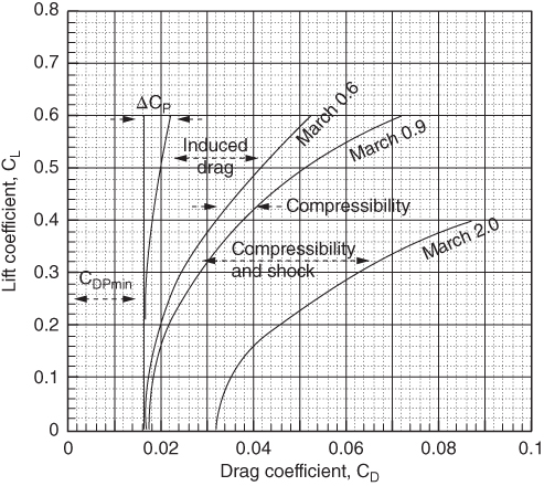
Figure 11.22 Vigilante RA C5 drag polar (not from industry).
Drag estimated at cruise altitude = 36 152 ft and Mach number = 0.6 (have compressibility drag).
Ambient pressure = 391.68 lb ft−2, Re/ft = 1.381 × 10⁶.
Design CL = 0.365, Design Mach number = 0.896 (Mcrit is at 0.9), Maximum Mach number = 2.0.
11.22.2 Computation of Wetted Areas, Re and Basic CF
The aircraft is first dissected into isolated components to obtain Re, the wetted area and the basic 2D flat plate CF of each component as listed next. Note that there is no correction factor for CF at Mach 0.6 (no compressibility drag). The CF compressibility correction factor (compute this from Figure 11.24b) at Mach 0.9 and Mach 2.0 will be applied later.
- Fuselage:

Figure 11.23 Drag comparison.
Fuselage wetted area = Awf = 1474 ft2
Fuselage Re = 69 × 1.381 × 106 = 9.53 × 10⁷ (length trimmed to what is pertinent for Re)
Use Figure 11.24, bottom graph to obtain basic CFf = 0.0021
- Wing
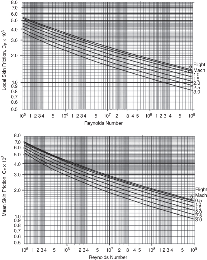
Figure 11.24 Flat pate skin friction coefficients versus Reynolds number (turbulent flow). (Top) Local skin friction. (Bottom) Mean skin friction.
Wing wetted area = Aww = 1144.08 ft2
Wing Re = 15.19 × 1.381 × 106 = 2.1 × 10⁷
Use Figure 11.24, bottom graph to obtain basic CFw = 0.00 257
- Empennage (same procedure as for wing)
V‐tail wetted area = AwVT = 235.33 ft2
V‐tail Re = 8.35 × 1.381 × 106 = 1.2 × 10⁷
Use Figure 11.24, bottom graph to obtain the basic CF_V‐tail = 0.00 277
H‐tail wetted area = AwHT = 3811.72 ft2.
H‐tail Re = 9.73 × 1.381 × 106 = 1.344 × 10⁷.
Use Figure 11.24, bottom graph to obtain basic CF_H‐tail = 0.002 705.
11.22.3 Computation of 3D and Other Effects to Estimate Component CDpmin
A component‐by‐component example is given next.
- Fuselage:
As before, at Mach 0.6, the basic CFf = 0.0021
3D effects (Eqs. 11.10–11.12):
Wrapping: ΔCFf = CFf × 0.025 × (length/diameter) × Re−0.2
- = 0.025 × 0.0021 × (9.66) × (9.53 × 107)‐0.2
- = 0.000 507 × 0.0254 = 0.0 000 129 (0.6% of basic CFf)
Supervelocity: ΔCFf = CFf × (diameter/length)1.5 = 0.0021 × (1/9.66)1.5
- = 0.0021 × 0.033 = 0.0 000 693 (3.3% of basic CFf)
Pressure: ΔCFf = CFf × 7 × (diameter/length)3 = 0.0021 × 7 × (0.1035)3
- = 0.0147 × 0.00 111 = 0.0 000 163 (0.8% of basic CFf)
Other effects on fuselage (this time intake has to be included – see Section ):
It is to be noted here that [3] suggests to apply a factor of 1.284 to include most of the other effects except for intake. Therefore, unlike the civil aircraft example, it is simplified to the following only:
Intake (little spillage – rest taken in 3D effects): 2%
Total ΔCFf increment is given in Table 11.21.
Table 11.21 Vigilante fuselage ΔCFf correction (3D and other shape effects).
| Item | ΔCFf | % of CFfbasic |
| Wrapping | 0.000 015 | 0.6 |
| Supervelocity | 0.000 1 | 3.3 |
| Pressure | 0.0 000 274 | 0.8 |
| Intake (little spillage) | 2 | |
| Total ΔCFf | 0.00 105 | 9.7 |
Therefore, in terms of equivalent flat plate area, f, it becomes = CFf × AwF.
Add canopy drag, CDπ = 0.08 (approximated from Figure 11.4).
Therefore canopy = 0.08 × 4.5 = 0.4 ft2. ffus = 3.3 + 0.36 = 3.66 ft2
- Wing:
From before, at Mach 0.06, the basic CF = 0.00 259.
3D effects (Eqs. 11.15–11.17):
Supervelocity: ΔCFw = CFw × 1.4 × (aerofoil thickness/chord ratio)
- = 0.00 257 × 1.4 × 0.05 = 0.00 018 (7% of basic CFw)
Pressure: ΔCFw = CFw × 60 × (aerofoil thickness/chord ratio)4× ![]()
- = 0.00 257 × 60 × (0.05)4 × (6/3.73)0.125
- = 0.1542 × 0.00 000 625 × 1.06 = 0.00 000 102 (0.04% of basic CFw)
Interference: ΔCFw for thin high wing take 3% of CFw.
Other effects:
Excrescence (non‐manufacturing, e.g. control surface gaps etc.):
| Flap/slat gaps | 2% |
| Others (increased later) | 0% |
| Total ΔCFw increment | 12.04% |
Table 11.22 summaries Vigilante wing ΔCFw correction (3D and other shape effects).
Table 11.22 Vigilante wing ΔCFw correction (3D and other shape effects).
| Item | ΔCFw | % of CFwbasic |
| Supervelocity | 0.000 385 | 7 |
| Pressure | 0.0 000 136 | 0.04 |
| Interference (wing‐body) | 0.0 000 328 | 3 |
| Flap/slat gap | 2 | |
| Total ΔCFw | 12.04 |
Therefore, in terms of equivalent flat plate area, f, it becomes = CFw × Aww
- Empennage
Since it follows the same procedure as in the case of wing, this is not repeated. The same percentage increment as the case of wing is taken as a classroom exercise. It may be emphasised here that in industry, one must compute systematically as shown in the case of wing.
V‐tail: Wetted area, AwVT = 235.33 ft2
- Basic CF_V‐tail = 0.00 277, fVT = 1.12 × 0.00 277 × 235.33 = 0.73 ft2
H‐tail: Wetted area, AwHT = 388.72 ft2
- Basic CF_H‐tail = 0.002 705, fHT = 1.12 × 0.002 705 × 388.72 = 1.18 ft2
11.22.4 Summary of Parasite Drag (ISA Day, 36 182 ft Altitude and Mach 0.9)
Wing reference area Sw = 700 ft2, CDpmin = f/Sw.
A Vigilante parasite drag summary is given in Table 11.23.
Table 11.23 Vigilante parasite drag summary.
| Fuselage | 3.66 ft2 |
| Wing | 3.3 ft2 |
| V‐tail | 0.73ft2 |
| H‐tail | 1.18 ft2 |
| Total | 8.87 ft2 |
As was indicated in Section 11.16 [3], offers a correlated factor of 1.284 to include all so‐called other effects. Therefore, the final flat plate equivalent drag faircraft = 1.284 × 8.87 = 11.39 ft2. 28.4% = 11.62 ft2 to include military aircraft excrescence.
It gives CDpmin at Mach 0.6 = 11.39/700 = 0.01 627 ([3] gives 0.1645, close enough).
This is the CDpmin at flight Mach number before compressibility effects start to show up, that is, it is seen as CDpmin at incompressible flow. At higher speed there is CF shift to a lower value. The CDpmin estimation needs to be repeated with lower CF at 0.9 Mach and at 2.0 Mach. To avoid repetition to account for compressibility, a factor of 0.97 (ratio of values at Mach 0.9 and Mach 0 in Figure 11.24, bottom graph – a reduction of 3%) is taken at 0.9 Mach. A factor of 0.8 (a reduction of 20%) is taken at 2.0 Mach as shown in Table 11.24. At compressible flow, add the wave drag. At supersonic speed it is contributed to by shock waves.
Table 11.24 Vigilante ΔCDp estimation.
| CL | 0 | 0.1 | 0.16 | 0.2 | 0.3 | 0.4 | 0.5 | 0.6 |
| ΔCDp | 0.000 8 | 0.00 015 | 0 | 0.000 1 | 0.000 8 | 0.00 195 | 0.003 6 | 0.006 |
To stay in line with the methodology presented here, the following values of ΔCDp have been extracted from [3].
11.22.5 ΔCDp Estimation
The data for ΔCDp given in Table 11.24 is extracted from Ref. [3] and is approximate.
11.22.6 Induced Drag
Formula used CDi = CL2/(3.14 × 3.73) = CL2/11.71.
The ΔCDi values used in Vigilante are given in Table 11.25.
Table 11.25 Vigilante induced drag.
| CL | 0.2 | 0.3 | 0.4 | 0.5 | 0.6 | 0.7 |
| CDi | 0.00 342 | 0.00 768 | 0.013 7 | 0.021 4 | 0.030 7 | 0.041 8 |
11.22.7 Supersonic Drag Estimation
Supersonic flight would have bow shock‐wave that is a form of compressibility drag, which is evaluated at zero CL. Drag increases with change of angle of attack. The difficulty arises in understanding the physics involved with increase in CL. Clearly, the increase, though lift dependent, has little to do with viscosity unless shock interacts with boundary layer to increase pressure drag. Since the very obligation of design is to avoid such interaction up to a certain CL, this book treats compressibility drag at supersonic speed as being composed of compressibility drag at zero CL (that is CD_shock) plus compressibility drag at higher CL (that is ΔCDw).
To compute compressibility drag at zero CL, the following empirical procedure is adopted, taken from [3]. Compressibility drag of an object depends on its thickness parameter, in case of the fuselage it is the fineness ratio and in case of wing it is the thickness to chord ratio. The fuselage (including the empennage) and wing compressibility drags are separately computed and then added along with the interference effects. Extensive use of graphs (Figures 11.25–11.31) is required for the empirical methodology. Compressibility drag values for both at Mach 0.9 and Mach 2.0 are estimated.

Figure 11.25 Corrections for laminarisation [3].

Figure 11.26 Supersonic compressibility drag [3].
Figure 11.27 Design‐lift coefficient [3].
Figure 11.28 Two‐dimensional drag divergence Mach number for supersonic aerofoil [3].

Figure 11.29 Design Mach number [3].
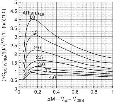
Figure 11.30 Supersonic wing compressibility drag [3].
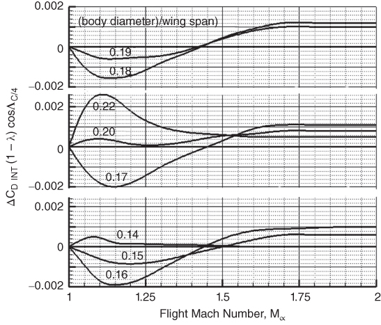
Figure 11.31 Wing‐body zero lift interference drag [3].
Drag estimation at Mach 0.9 follows the same method as worked out in the civil aircraft example and is tabulated in Section 11.19.
Fuselage compressibility drag (includes empennage contribution) at Mach 2.0:
Thickness parameter is fuselage fineness ratio.
- Step 1. Plot fuselage cross‐section along fuselage length as shown in Figure 11.22 and obtain the maximum cross‐section, Sπ = 45.25 ft2 and the fuselage base Sb = 12 ft2. Find the ratio
- Find (1 + Sb/Sπ) = 1 + 12/45.25 = 1.27.
- Find Sπ/Sw = 45.25/700 = 0.065.
- Step 2. Get the fuselage fineness ratio l/d = 73.3/7.788 = 9.66 (d is minus intake width).
- Obtain (l/d)2 = (9.66)2 = 93.3.
- Step 3. Use Figure 11.26 to get CDπ(l/d)2 = 18.25 at M∞ = 2.0 for (1 + Sb/Sπ) = 1.27
- This gives CDπ = 18.25/93.3 = 0.1956.
- Convert this to the fuselage contribution of compressibility drag expressed in terms of wing reference area, CDwf = CDπ × (Sπ/Sw) = 0.1956 × 0.065 = 0.01 271.
Wing compressibility drag at Mach 2.0:
- Step 1. Obtain design CL_DES from Figure 11.27 for supersonic aerofoil for
- AR × (t/c)⅓ = 3.73 × (0.05)⅓ = 1.374. It gives CL_DES = 0.352.
- Test data of CL_DES from [3] gives 0.365, which is close enough. Test data is used.
- Step 2. Obtain from Figure 11.28 the two‐dimensional design Mach number, MDES_2D = 0.784.
- Using Figure 11.29 obtain ΔMAR = 0.038 for 1/AR = 0.268.
- Using Figure 11.29 obtain ΔMDΛ¼ = 0.067 for Λ¼ = 37.5°.
- Step 3. Make the correction to get design Mach as MDES = MDES_2D + ΔMAR + ΔMDΛ¼.

- Then ΔM = M∞ − MDES = 2.0 − –0.889 = 1.111.
- Step 4. Compute (t/c)5/3 × [1 + (h/c)/10)] = (0.05)5/3 × [1 + (0)/10)] = 0.00679.
- Step 5. Compute ARtan ΛLE = 3.73 × tan43 = 3.73 × 0.9325 = 3.48.
- Step 6. Use Figure 11.30 and the corresponding value of ARtan ΛLE = 3.48 in Step 5.

- Compute ΔCDC_WING = 0.675 × 0.00 679 = 0.00458
Finally, interference drag at supersonic speed has to be added to fuselage and wing compressibility drag.
The procedure for estimating wing‐fuselage interference drag is given next.
- Step 1. Compute (fuselage diameter at maximum area/wing span) = 7.785/53.14 = 0.1465
- Step 2. With a taper ratio, λ = 0.19, compute (1 − λ)cosΛ¼ = (1 − 0.19) cos37.5 = 0.643.
- Step 3. Using Figure 11.31 obtain ΔCD_INT × [(1 − λ)cosΛ¼] = 0.00 048
- Compute ΔCD_INT = 0.00 048/0.643 = 0.00 075.
Summary of compressibility drag of a Vigilante at zero lift
Compressibility drag at Mach 0.6 (3% reduction on account CF change) and Mach 0.9 (20% reduction on account CF change) has been done as in the case of a civil aircraft and is given in Table 11.26 along with drag at Mach 2.0.
Table 11.26 Vigilante supersonic drag summary.
| CDw at Mach 2.0 | |
| Fuselage/empennage contribution | 0.01 271 |
| Wing contribution | 0.00 458 |
| Wing‐fuselage interference (supersonic only) | 0.00 075 |
| Total | 0.01 804 |
11.22.8 Total Aircraft Drag
Total Vigilante drag at the three Mach numbers is tabulated in Table 11.27. Figure 11.8 gives the Vigilante drag polar at the three aircraft speeds. Figures 11.24–11.31 are re‐plotted in this chapter from [3].
Table 11.27 Vigilante total aircraft drag coefficient, CD.
| At Mach 0.6 | |||||||
| CL | 0.0 | 0.1 | 0.2 | 0.3 | 0.4 | 0.5 | 0.6 |
| CDpmin | 0.01 627 | ||||||
| ΔCDp | 0.000 8 | 0.00 015 | 0.000 1 | 0.000 8 | 0.00 195 | 0.003 6 | 0.006 |
| CDi | 0 | 0.000 854 | 0.00 342 | 0.00 768 | 0.013 7 | 0.021 4 | 0.030 7 |
|
Aircraft CD @ Mach 0.6 |
0.01 707 | 0.01 727 | 0.019 8 | 0.02 475 | 0.03 192 | 0.04 127 | 0.052 3 |
| At Mach 0.9 | |||||||
| CL | 0.0 | 0.1 | 0.2 | 0.3 | 0.4 | 0.5 | 0.6 |
| CDpmin | 0.97 × 0.01 627 = 0.01 582 (Ref [3] gives 0.01 575) | ||||||
| ΔCDp | 0.000 8 | 0.00 015 | 0.000 1 | 0.000 8 | 0.00 195 | 0.003 6 | 0.006 |
| CDi | 0 | 0.000 854 | 0.00 342 | 0.00 768 | 0.013 7 | 0.021 4 | 0.030 7 |
| Wave drag, CDw | 0.000 3 | 0.001 | 0.002 | 0.003 2 | 0.005 5 | 0.01 | 0.02 |
|
Aircraft CD @ Mach 0.9 |
0.01 737 | 0.01 827 | 0.021 8 | 0.02 795 | 0.03 742 | 0.05 127 | 0.072 3 |
| CDw versus CL is to be taken from CFD/test data. Here it is reduced from Ref. [3] | |||||||
| At Mach 2.0 | |||||||
| CL | 0.0 | 0.1 | 0.2 | 0.3 | 0.4 | 0.5 | 0.6 |
| CDpmin | 0.8 × 0.01 627 = 0.013 (Ref [3] gives 0.01302) | ||||||
| ΔCDp | 0.000 8 | 0.00 015 | 0.000 1 | 0.000 8 | 0.00 195 | 0.003 6 | 0.006 |
| CDi | 0 | 0.000 854 | 0.00 342 | 0.00 768 | 0.013 7 | 0.021 4 | 0.030 7 |
| Shock drag | 0.01 804 at zero CL (CD_shock) | ||||||
| Wave drag, ΔCDw | 0.0 | 0.003 | 0.011 | 0.023 | 0.041 | ||
|
Aircraft CD @ Mach 2.0 |
0.031 8 | 0.035 | 0.045 5 | 0.062 5 | 0.087 | ||
ΔCDw versus CL is to be taken from CFD/test data.
11.23 Drag Comparison
The following equations are the parabolic drag polar of the aircraft used as classwork examples. Figure 11.23 compares the drag polar values of the Bizjet, the AJT and the TPT.
Bizjet: (Oswald efficiency factor, e, determined in Section 4.9.3.).
Classwork example: Bizjet drag may be approximated as parabolic drag polar as given here.
(gives Oswald's efficiency factor, e = 0.95)
AJT: (Reader's to work out the Oswald efficiency factor, e).
Classwork example AJT drag may be approximated as parabolic drag polar as given here.
(gives Oswald's efficiency factor, e = 0.85)
Turboprop (TPT): (low‐speed aircraft – Oswald efficiency factor, e, fits closely with actual polar).
Maximum TPT speed is below 0.5 Mach (incompressible flow). Here parabolic drag is close enough to actual drag polar.
(gives Oswald's efficiency factor, e = 0.875)
Figure 11.23 compares actual drag polar with parabolic drag polar for the three classwork examples, that is, the Bizjet, the TPT and the AJT. It may be noted that the three graphs are close enough within the operating range below Mcrit. Equation (10.5) represents typical high speed subsonic aircraft operational segments of LRC, en‐route climb and descent. The TPT flies in incompressible flow region and parabolic drag polar can be used to get good results. At HSC, non‐linear effects show up. The Bizjet and AJT operate in high subsonic at Mcrit and, therefore, semi‐empirically determined actual drag polar is the preferred one. This is the standard procedure practised in industry, which gives credible output as well as offering the entire characteristics by close‐form solutions.
11.24 Some Concluding Remarks
It is emphasised that, unlike the other chapters, this important chapter has some concluding remarks. Drag estimation is a state‐of‐the‐art and covers a very large territory, as can be seen in this chapter. There is a tendency to underestimate drag primarily on account of missing out some of the multitude of items those need to be considered in the process of estimation.
The object of this chapter is to make readers aware of the sources of drag as well as give a methodology in line with typical industrial practices (without CFD results). Some of the empirical relations are guesstimates based on industrial data available to the authors; those are not in the public domain. The formulation could not possibly cover all aspects of drag estimation methodologies and therefore has to be simplified for classroom usage. For example, the drag of high‐lift devices could only give ballpark figures.
Readers are advised to rely on industrial data or generate their own data bank through CFD/tests. The authors would be grateful to receive data and/or substantiated formulation on these that could improve accuracy in future editions (with due acknowledgement).
References
- 1. Hoerner, S. F. Fluid Dynamic Drag, Bricktown, NJ: Published by published by the author. 1965.
- 2. AGARD LS 67 – Prediction Method for Aircraft Aerodynamic Characteristics, 1974.
- 3. Feagan, R.C. and Morrision, W.D. (1978). Delta Method – An Empirical Drag Build‐Up Technique. Lockheed California Company. NASA Contractor Report 151 971.
- 4. USAF. USAF Data Compendium for Stability and Control (DATCOM). https://ipfs.io/ipfs/QmXoypizjW3WknFiJnKLwHCnL72vedxjQkDDP1mXWo6uco/wiki/USAF_Stability_and_Control_DATCOM.html.
- 5. ESDU. (2012). 90029, An Introduction to Aircraft Excrescence Drag, London.
- 6. Kundu, A.K., Price, M.A., and Riordan, D. (2016). Theory and Practice of Aircraft Performance. John Wiley & Sons, Ltd. ISBN: ISBN: 9871119074175.
- 7. Kundu, A.K. (2010). Aircraft Design. Cambridge University Press. ISBN: ISBN: 978‐0‐521‐88516‐4.
- 8. Kundu, A. K. Subsonic aircraft drag estimation. Shorts Document No: AR/0001, October 1995 (not in public domain).
- 9. Aerodynamic Drag, AGARD CP 124. 7 Rue Ancelle, F‐92200 Neuilly‐sur‐Seine, France, April 1973.
- 10. AGARD AR 256. (1989). Technical status review on drag prediction and analysis from Computational fluid dynamics: State‐of‐the‐art.
- 11. Torenbeek, E. (1982). Synthesis of Subsonic Airplane Design. Springer.
- 12. Haines, A.B. (1968). Subsonic aircraft drag: an appreciation of present standards. Aeronautical Journal 72, No. 687.
- 13. Young, A.D. and Paterson, J.H. (1981). *AGARD AG264 Aircraft excrescence drag. 7 Rue Ancelle, F‐92200 Neuilly‐sur‐Seine, France.
- 14. Seddon, J. and Goldsmith, E. (1965). Practical Intake Aerodynamic Design. Reston, VA: AIAA.
- 15. Farokhi, S. (1991). Propulsion System Integration. Short Course. Lawrence, KS: University of Kansas.
- 16. Kundu, A.K., Watterson, J., MacFadden, R. et al. (2002). Parametric optimisation of manufacturing tolerances at the aircraft surface. Journal of Aircraft 39, No 2, AIAA.