17
Aircraft Load
17.1 Overview
Aircraft performance depends on its structural integrity to withstand the design load level. Aircraft structures must withstand the imposed load during operations; the extent depends on what is expected from the intended mission role. The higher the load, the heavier the structure for its integrity; hence the maximum takeoff weight (MTOW) affecting aircraft performance. Aircraft designers must comply with the mandatory certification regulations to meet the minimum safety standards.
The information provided herein is essential for understanding performance considerations that affect aircraft mass (i.e. weight), hence its performance. The V‐n diagram depicts the loading condition and the limits of aircraft flight envelope. Only the loads and associated V‐n diagram in symmetrical flight are discussed herein. Estimation of load is a specialised subject covered in focused courses and textbooks [1, 2]. However, this chapter does outline the key elements of aircraft loads.
This chapter includes the following sections:
- Section 17.2: Introduction to Aircraft Load, Buffet and Flutter
- Section 17.3: Flight Manoeuvres
- Section 17.4: Aircraft Load
- Section 17.5: Theory and Definitions (Limit and Ultimate Load)
- Section 17.6: Limits (Load Limit and Speed Limit)
- Section 17.7: V‐n Diagram (the Safe Flight Envelope)
- Section 17.8: Gust Envelope
Classwork content. The chapter can be skipped if the subject has been learned about in other coursework, otherwise the readers must go through it.
17.2 Introduction
Loads are the external forces applied to an aircraft in its static or dynamic state of existence, in‐flight or on‐ground. In‐flight loads are due to symmetrical flight, unsymmetrical flight or atmospheric gusts from any direction. On‐ground loads result from ground handling and field performance (e.g. in static, takeoff and landing). Aircraft designers must be aware of the applied aircraft loads, ensuring that configurations are capable of withstanding them. The subject matter concerns the interaction between aerodynamics and structural dynamics (i.e. deformation occurring under load), a subject that is classified as aeroelasticity. Even the simplified assumption of an aircraft as an elastic body requires study beyond the scope of this book. This book addresses rigid aircraft, explained in Section 4.1.
User specifications define the manoeuvre types and speeds that influence aircraft weight, which then dictates aircraft design, affecting aircraft performance. In addition, enough margin must be allocated to cover inadvertent excessive load encountered through pilot‐induced manoeuvres, or sudden severe atmospheric disturbances (i.e. external input) or a combination of the two scenarios. The limits of these inadvertent situations are derived from historical statistical data and pilots must avoid exceeding the margins. To ensure safety, governmental regulatory agencies have mandatory requirements for structural integrity specified with minimum margins. Load factor (not to be confused with the passenger load factor) is a term that expresses structural‐strength requirements. The structural regulatory requirements are associated with V‐n diagrams, which are explained in Section 17.7. In fact, they also require mandatory strength tests to determine ultimate loads, which must be completed before the first flight, with the exceptions of homebuilt and experimental categories of aircraft. In the following sections, buffet and flutter are introduced.
17.2.1 Buffet
The buffet phenomenon occurs at the insipient phase of stall at low-speed 1‐g level flight. Actually buffet can occur at any speed, whenever flow instability over the wing takes place, for example, during extreme manoeuvres, at higher g loads (n > 1) when the angle of attack increases to high values. Buffet can also occur at 1‐g high‐speed (called Mach buffet) when transonic flow over‐wing (or over any other lifting surface) local shocks interact with the boundary layer to cause unstable separation making the airflow over the wing unsteady; the separation line over the wing keeps fluctuating. In this situation, the H‐tail can also get induced to start buffeting. This causes the aircraft to shudder and is a warning to the pilot. The aircraft structure is not necessarily at its maximum loading.
It is clear that every class of aircraft has two stall speeds, hence there are two buffet speeds; one low‐speed buffet and the other a Mach buffet at high‐speed, the magnitude depends on its weight, altitude and ambient conditions (Figure 17.1). At higher altitudes, because of lower air density, the low‐speed buffet goes up while the Mach buffet speed goes down. Low‐speed stall buffet is based purely on aircraft aerodynamic design but the high‐speed Mach buffet requires the additional requirement of engine capability to attain such speeds in level flying. The excess available thrust between the two limits allows the aircraft to climb. Where the two buffet limit lines merge is the aerodynamic aircraft aerodynamic ceiling height, when the rate of climb reaches zero.

Figure 17.1 Typical buffet boundary.
17.2.1.1 Q‐Corner – (Coffin Corner)
As the aircraft reaches the aerodynamic ceiling, the buffet margin between the low‐speed and high‐speed range gradually gets reduced and it becomes very difficult to fly in this small margin. Flying slower will make the aircraft stall and when flying faster, the aircraft starts shuddering. At low‐speed stall, the aircraft nose drops and gains speed only to enter into high‐speed buffet shudder. If delayed to take recovery action, then control problems may arise and can pose problems in recovery. This zone is loosely termed the ‘coffin corner’ (Q‐corner). Aircraft flight in this zone is carried out but only by test pilots in order to establish the buffet boundary to be aware of. Operational flying stays away from the buffet boundary. However, there are exceptions for special missions, for example, the reconnaissance aircraft Lockheed U2 was designed to fly at high altitudes near its ceiling to stay out of missile reach at that time. The Lockheed U2 has a less than 1% margin between low and high speed (within the Q‐corner) at either side of the onset of aircraft buffeting. Civil aircraft regulation requires that aircraft should fly 30% below CLbuffet. The buffet ‘g’ should not exceed this limit (see Table 17.1). This also gives a margin for the pilot to manoeuvre to a ‘g’ level of n = 1.3. Although known as the coffin corner, as such, it is not dangerous to fly if pilot can recognise the incipient stage of buffet onset and the 30% margin allows manoeuvring to recover. It is possible the term originated from a different reason than being dangerous to fly – it is better to use the term Q‐corner.
Table 17.1 Typical permissible g‐load for civil aircraft.
| Type | Ultimate positive n | Ultimate negative n |
| FAR25 (14CFR25) | ||
| Transport aircraft below 50 000 lb | 3.75 | −1 to −2 |
| Transport aircraft above 50 000 lb | [2.1 + 24 000/(W + 10 000)] | −1 to −2 |
| Should not exceed 3.8 | ||
| FAR23 (14CFR23) | ||
| Aerobatic category (FAR23 only) | 6 | −3 |
The sized engine should have a maximum cruise rating thrust capability to reach the ceiling altitude for the aircraft weight. The absolute aircraft ceiling is actually when rated (normally maximum cruise rating) thrust limited speed equals the stall speed at the aircraft weight, when the aircraft rate of climb is zero: a point could be below high‐speed Mach buffet. At a higher thrust rating, say at a maximum continuous rating, the aircraft will have some excess thrust to climb, possibly, limited by high‐speed Mach buffet until it reaches the stall buffet at the Q‐corner when the aircraft ceases to climb reaching the aerodynamic ceiling for the weight. Any further thrust increase is of no use as the aircraft is already limited by the buffet lines from both sides. Also, note in Figure 17.1 the structural limit line of VMO at 0.81 Mach. The aircraft does not have the capability to reach VMO in level flight but it is possible in a dive. At low altitudes the VMO is given at constant equivalent airspeed (EAS) (in this example 330 kt until it reaches 0.81 Mach at around 27 000 ft altitude) when the structural speed limit is below high‐speed Mach buffet limit. At low altitudes, a civil aircraft has no operational role to operate at such a high speed. At cruise altitude, the aircraft is cruise thrust limited (Figure 17.1) and stays below high‐speed Mach buffet limit. Military aircraft operate differently but have to fly below their structural limits as well as avoid buffeting.
The buffet boundary for each class of aircraft has to be established for the full flight envelope. At the design stage, simulation analyses can give a preliminary indication of buffet boundary, followed by wind‐tunnel tests to serve as guidelines for the pilot to establish the buffet boundary through flight tests for operational usage. Typically, combat aircraft are allowed to tolerate higher levels of buffet compared to transport aircraft for operational reasons. The aircraft design must be free from Mach buffet within the operational envelope.
In the Federal Aviation Administration (FAA) regulations, establishing buffet boundary is a flight test task. The pass/fail assessment is made by the approved test pilot and is solely the result of the pilot's experience and judgement. These data are proprietary information kept commercial in confidence. It is difficult to find examples to give a worked‐out example. The readers may contact aircraft manufacturers to get a proper buffet boundary with explanations. An Internet search for the FAA website graphs may give some indications.
17.2.2 Flutter
This is the vibration of the structure that may cause deformation; primarily the wing, but also any other component depending on its stiffness. At transonic speed, the load on the aircraft is high while the shock‐boundary layer interaction could result in an unsteady flow causing vibration of the wing, for example. The interaction between aerodynamic forces and structural stiffness is the source of flutter. A weak structure enters into flutter; in fact, if it is too weak, flutter could happen at any speed because the deformation would initiate the unsteady flow. If it is in resonance, then it could be catastrophic – such failures have occurred. Flutter is an aeroelastic phenomenon, while buffet is not. Aircraft flutter is dangerous and must be avoided. At design stage, simulation analyses can give preliminary indication of flutter speed, followed by wind‐tunnel tests to improve accuracy followed by flight test substantiation. Being dangerous, flight tests are carried out under utmost caution.
17.3 Flight Manoeuvres
Although throttle‐dependent linear acceleration would generate flight load in the direction of the flight path, pilot‐induced control manoeuvres could generate the extreme flight loads that may be aggravated by inadvertent atmospheric conditions. Aircraft weight is primarily determined by the air load generated by manoeuvres in the pitch plane. The associated V‐n diagram described in Section 17.7 provides useful information for aircraft performance analysis. Section 3.6.1 describes the six degrees of freedom for aircraft motion – three linear and three angular. Given here are the three Cartesian coordinate planes of interest.
17.3.1 Pitch‐Plane (x–z‐Plane) Manoeuvre: (Elevator/Canard Induced)
The pitch plane is the symmetrical vertical plane (i.e. x–z‐plane) in which the elevator/canard‐induced motion occurs with angular velocity, q, about the y‐axis, in addition to the linear velocities in the x–z‐plane. Changes in the pitch angle due to angular velocity q results in changes in CL. The most severe aerodynamic loading occurs in this plane.
17.3.2 Roll‐Plane (y–z‐Plane) Manoeuvre: (Aileron Induced)
The aileron‐induced motion generates the roll manoeuvre with angular velocity, p, about the x‐axis, in addition to velocities in the y–z‐plane. Roll‐plane loading is not discussed here.
17.3.3 Yaw‐Plane (y–x‐Plane) Manoeuvre: (Rudder Induced)
The rudder‐induced motion generates the yaw (coupled with the roll) manoeuvre with angular velocity, r, about the z‐axis, in addition to the linear velocities in the y–x‐plane. Aerodynamic loading of an aircraft due to yaw is also necessary for structural design. It is not discussed here.
17.4 Aircraft Loads
An aircraft is subject to load at any time. The simplest case is an aircraft stationary on the ground experiencing its own weight. Under heavy landing, an aircraft can experience severe loading and there have been cases of structural collapse. Most of these accidents showed failure of the undercarriage, but breaking of the fuselage also has occurred.
h3
17.4.1.1 On‐Ground
Loads on the ground are taken up by the undercarriage and then transmitted to the aircraft main structure. Landing gear loads are dependent on the specification of Vstall, the maximum allowable sink speed rate at landing and on the maximum takeoff mass (MTOM). The topic is dealt with in greater detail in Chapter 9 concerning undercarriage layout for conceptual study.
17.4.1.2 In Flight
In flight, aircraft loading varies with manoeuvres and/or when gusts are encountered. Early designs resulted in many structural failures in operation. In‐flight loading in the pitch plane is the main issue considered in this chapter. The aircraft structure must be strong enough at every point to withstand the pressure field around the aircraft, along with the inertial loads generated by flight manoeuvres. The V‐n diagram is the standard way to represent the most severe flight loads that occur in the pitch plane (i.e. the x–z plane).
Civil aircraft designs have conservative limits; there are special considerations for the aerobatic category of aircraft. Military aircraft have higher limits for hard manoeuvres and there is no guarantee that, under threat, a pilot would be able to adhere to the regulations. Survivability requires widening the design limits and strict maintenance routines to ensure structural integrity. Typical human limits are currently taken at 9 g in sustained manoeuvres and can reach 12 g for instantaneous loading. Continuous monitoring of the statistical database retrieved from aircraft‐mounted black boxes provides feedback to the next generation of aircraft design or at midlife modifications. A g‐meter in the flight deck records the g‐force and a second needle remains at the maximum g reached in the sortie. If the prescribed limit is exceeded, then the aircraft must be grounded for a major inspection. An important aspect of design is to know what could happen at the extreme points of the flight envelope (i.e. the V‐n diagram).
17.5 Theory and Definitions
In steady, level flight, an aircraft is in equilibrium; that is, the lift, L, equals the aircraft weight, W, and the thrust, T, equals drag, D. The wing produces all the lift with a spanwise distribution (see Section 5.4.9). In equation form, for steady level flight:
17.5.1 Load Factor, n
Newton's law states that change from an equilibrium state requires an additional applied force, that would associate with some form of acceleration, a. When applied in the pitch plane to increase the angle of incidence, α, initiated by rotation of the aircraft, the additional force appears as an increment in lift, ΔL, resulting in gain in height (Figure 17.2).
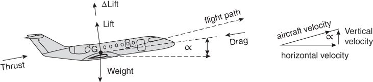
Figure 17.2 Equilibrium flight.
From Newton's law,
The resultant force equilibrium gives
Load factor, n, is defined as
The load factor, n, indicates the increase in force contributed by the centrifugal acceleration, a. The load factor, n = 2, indicates a two‐fold increase in weight; that is, a 90‐kg person would experience a 180‐kg weight. The load factor, n, is loosely termed the g‐load; in this example, it is the 2‐g load. Unaccelerated normal force on a body is its weight.
A high g‐load damages the human body, with the human limits of the instantaneous g‐load higher than for continuous g‐loads. For a fighter pilot, the limit (i.e. continuous) is taken as 9‐g; for the civil aerobatic category, it is 6‐g. Negative g‐loads are taken as half of the positive g‐loads. Fighter pilots use pressure suits to control blood flow (i.e. delay blood starvation) to the brain to prevent ‘blackouts’. A more inclined pilot seating position reduces the height of the carotid arteries to the brain, providing an additional margin on the g‐load that causes a blackout.
Because they are associated with pitch‐plane manoeuvres, pitch changes are related to changes in the angle of attack, α, and the velocity, V. Hence, there is variation in CL, up to its limit of CLmax, in both the positive and negative sides of the wing incidence to airflow. The relationship is represented in a V‐n diagram (Figure 17.3). Atmospheric disturbances are natural causes that appear as a gust load from any direction. Aircraft must be designed to withstand this unavoidable situation up to a statistically determined point that would encompass almost all‐weather flights, except extremely stormy conditions. Based on the sudden excess in loading that can occur, margins are built in; as explained in the next section.
17.6 Limits – Load and Speeds
Limit load is defined as the maximum load that an aircraft can be subjected to in its life cycle. Under the limit load, any deformation recovers to its original shape and would not affect structural integrity. Structural performance is defined in terms of stiffness and strength. Stiffness is related to flexibility and deformations and has implications for aeroelasticity and flutter. Strength concerns the loads that an aircraft structure is capable of carrying and is addressed within the context of the V‐n diagram.
To ensure safety, a margin (factor) of 50% increase is enforced through regulations as a factor of safety to extend the limit load to the ultimate load. A flight load exceeding the limit load but within the ultimate load should not cause structural failure but could affect integrity with permanent deformation. Aircraft are equipped with g‐meters to monitor the load factor – the n for each sortie – and, if exceeded, the airframe must be inspected at prescribed areas and maintained by prescribed schedules that may require replacement of structural components. For example, an aerobatic aircraft with a 6‐g‐limit load will have an ultimate load of 9 g. If an in‐flight load exceeds 6 g (but is below 9 g), the aircraft may experience permanent deformation but should not experience structural failure. Above 9 g, the aircraft would most likely experience structural failure.
The factor of safety also covers inconsistencies in material properties and manufacturing deviations. However, aerodynamicists and stress engineers should calculate for load and component dimensions such that their errors do not erode the factor of safety. Geometric margins, for example, should be defined such that they add positively to the factor of safety.
For civil aircraft applications, the factor of safety equals 1.5 (FAR 23 (14CAR23) and FAR 25 (14CAR 25), Vol. 3).
17.6.1 Maximum Limit of Load Factor, n
This is the required manoeuvre load factor at all speeds up to VC. (The next section defines speed limits.) Maximum elevator deflection at VA and pitch rates from VA to VD must also be considered. Table 17.2 gives the g‐limit of various aircraft classes.
Table 17.2 Typical g‐loads for classes of aircraft.
| Club flying | Sports aerobatic | Transport | Fighter | Bomber |
| +4 to −2 | +6 to −3 | 3.8 to −2 | +9 to −4.5 | +3 to −1.5 |
Military Aircraft (Military Specification MIL‐A‐8860, MIL‐A‐8861 and MIL‐A‐8870)
In general, there is factor of safety = 1.5 but this can be modified through negotiation. The g‐levels taken here are instantaneous limits based on typical human capability.
17.7 V‐n Diagram
To introduce the V‐n diagram, the relationship between load factor, n, and lift coefficient, CL, must be understood. The fundament flight operational domain is termed the ‘manoeuvre’ envelope. The V‐n envelope also includes the domain termed the ‘gust envelope’, covering the atmospheric disturbances from statistical weather data that are seen as all‐weather conditions, except some extreme situations that must be avoided for operation. An aircraft must be able to perform safely with these two boundaries of speed and load it encounters.
Pitch‐plane manoeuvres result in the full spectrum of angles of attack at all speeds within the prescribed boundaries of limit loads. Since CL varies with changes in attitude and/or aircraft weight, the V‐n diagram for each altitude and/or weight will be different. Typically, the specification is given at MTOM and sea level at the STD condition. The V‐n diagram is established out at the specified weight and altitude for detailed analyses. The V‐n diagram is constructed for the critical altitude, typically at 20 000 ft at its maximum weight at that altitude. In principle, it may be necessary to construct several V‐n diagrams representing different altitudes.
Depending on the direction of pitch‐control input, at any given aircraft speed, positive or negative angles of attack may result. The control input would reach either the CLmax or the maximum load factor n, whichever is the lower of the two. The higher the speed, the greater the load factor, n. Compressibility has an effect on the V‐n diagram. This chapter explains the role of the V‐n diagram to understand aircraft manoeuvre performance only in the pitch plane.
Figure 17.3 represents a typical V‐n diagram showing varying speeds within the specified structural load limits. The figure illustrates the variation in load factor with airspeed for manoeuvres. Some points in a V‐n diagram are of minor interest to configuration studies – for example, at the point V = 0 and n = 0 (e.g. at the top of the vertical ascent just before the tail slide can occur). Inadvertent situations may take aircraft from within the limit‐load boundaries to conditions of ultimate load boundaries. The points of interest are explained in the remainder of this section.

Figure 17.3 A typical V‐n diagram showing load and speed limits (pitch plane).
17.7.1 Speed Limits
The V‐n diagram (Figure 17.4) described in the next section uses various speed limits as defined here [2]. More details of the speed definitions are given in Section 17.8.
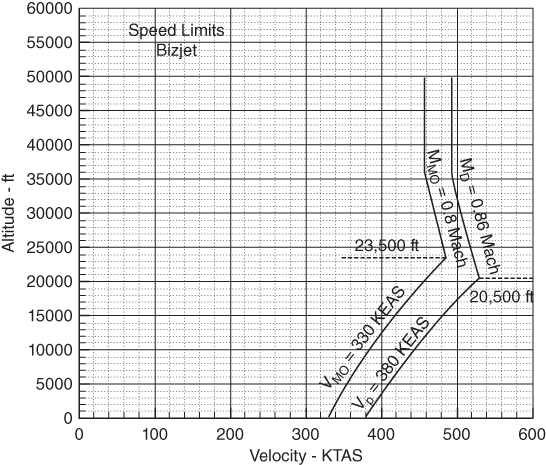
Figure 17.4 Bizjet speed limits.
VS – Stalling speed at normal level flight.
VA – Design manoeuvring speed. FAR (14CFR) specifies, VA = VS√n. Stalling speed at limit load. In a pitch manoeuvre, an aircraft stalls at a higher speed than vS. In an accelerated manoeuvre of pitching up, the angle of attack, α, reduces and hence stalls at higher speeds. The tighter the pitch manoeuvre, the higher the stalling speed until it reaches VA.
VB – Stalling speed at maximum gust velocity. This is the design speed for maximum gust intensity.
The speed should not be less than VB = VS√(ngust @ VC).
VC – Maximum design cruising (level) speed. Typically, VC ≥ VB + 43 kt. This serves as safety margin (not dealt in this book) above VB. VC is the specified operating condition. See Table 17.3 for the relation between VC and the positive/negative vertical gust velocity at altitudes.
Table 17.3 FAR (14CFR) Part 217.341a Specified gust velocity (in EAS).
| Altitude | 20 000 ft and below | Altitudes 20 000 ft and above |
| VB (rough air gust – maximum) | 66 ft s−1 | Linear reduction to 38 ft s−1 at 50 000 ft |
| VC (gust at max design speed) | 50 ft s−1 | Linear reduction to 25 ft s−1 at 50 000 ft |
| VD (gust at max dive speed) | 25 ft s−1 | Linear reduction to 12.5 ft s−1 ft s−1 at 50 000 ft |
VD – maximum permissible speed (occurs in dive – sometimes known as placard speed) – structural limitation.
VF – Design flap speeds. (Separate V‐n diagram. This is dealt with in this book.)
An aircraft can fly below stall speed if it is in a manoeuvre that compensates loss of lift, or the aircraft attitude is below the maximum angle of attack, αmax, for stalling.
Bizjet example
VS = 82.6 KEAS, VC = 328.6 KEAS, VA = 180 KEAS (see next)
VMO = 330 KEAS < 24 000 ft altitude, 0.8 Mach ≥ 23 500 ft
VD = 380 KEAS < 21 000 ft altitude, 0.86 Mach ≥ 20 500 ft
17.7.2 Extreme Points of the V‐n Diagram
Following the corner points of the flight envelope (Figure 17.5) is of interest for the stress and performance engineers. Beefing up of structures would establish an aircraft weight that must be predicted at the conceptual design phase. It also indicates the limitation points of the flight envelope in the pitch plane.

Figure 17.5 Aircraft angles of attack in pitch plane manoeuvres (see text for the abbreviations).
Figure 17.5 shows the various attitudes in pitch plane manoeuvres associated with the V‐n diagram, each of which are explained next. Note that manoeuvre is a transient situation. The various positions of Figure 17.5 can occur under more than one possibility. Only the attitudes associated by the predominant cases in pitch plane are outlined. Negative g occurs when the manoeuvre force is directed in the opposite direction towards the pilot's head, irrespective of his/her orientation with respect to the Earth.
17.7.2.1 Positive Loads
This is when the aircraft (and occupants) experiences force greater than its normal weight. Aircraft stalls at manoeuvres reaching αmax. The following lists the various possibilities. In level flight at 1 g, aircraft angle of attack, α, increases with deceleration and reaches its maximum value, αmax; the aircraft would stall at a speed vS.
- Positive High Angle of Attack (+PHA). This occurs at pull up manoeuvre raising the aircraft nose in a high pulling g‐force reaching the limit. The aircraft could stall if pulled harder. At a limit load of ‘n’ the aircraft reaches +PHA at aircraft speeds of VA.
- Positive Intermediate Angle of Attack (+PIA). This occurs at high‐speed level flight when control is actuated to set wing incidence at an angle of attack. Noting that the aircraft has maximum operating speed limit of VC, when +PIA reaches at the maximum limit load of n in manoeuvre – it is in transition or held at an intermediate level of manoeuvre.
- Positive Low Angle of Attack (+PLA). This occurs when the aircraft gains maximum allowable speed, sometimes in a shallow dive (dive speed, VD) and then at very small elevator pull (low angle of attack) would hit the maximum limit load of n. Some high powered military aircraft can reach VD at level flight. The higher the speed, the lower the angle of attack, α, would be to reach the limit load – at the highest speed, it would have +PLA.
17.7.2.2 Negative Loads
This occurs when an aircraft (and occupants) experiences forces less than its weight. In an extreme manoeuvre, in bunt (developing −ve g in a nose down curved trajectory), the centrifugal force pointing away from the centre of the Earth can cancel weight when the pilot feels weightless during the manoeuvre. The corner points follow the same logic of the positive load description except that the limit load of n is in the negative side, which is lower due to not being in normal flight regimes. It can occur during aerobatic flight, in combat or in inadvertent situation through atmospheric gusts.
- iv. Negative High Angle of Attack (−NHA). This is the inverted situation of case (i) explained before. With negative g it has to be in a manoeuvre.
- v. Negative Intermediate Angle of Attack (−NIA). This is the inverted situation of case (i). The possibility of negative α was mentioned when the elevator is pushed down, called a ‘bunting’ manoeuvre. Negative α classically occurs at inverted flight at the highest design speed, VC (coincided with PIA). When it reaches the maximum negative limit load of n, the aircraft takes NIA.
- vi. Negative Low Angle of Attack (−NLA). This is the inverted situation of case (iii). At VD, the aircraft should not exceed zero g.
17.7.3 Low‐Speed Limit
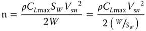
At low speeds, the maximum load factor is constrained by the aircraft CLmax. The low‐speed limit in a V‐n diagram is established at the velocity at which the aircraft stalls in an acceleration flight load of n until it reaches the limit‐load factor. At higher speeds, the manoeuvre load factor may be restricted to the limit‐load factor, as specified by the regulatory agencies. The V‐n diagram is constructed with VEAS representing the altitude effects.
Let VS1 be the stalling speed at 1 g then

or
or

This gives,

In manoeuvre, let VSn be the stalling speed at load factor, n,then
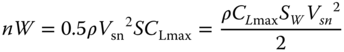
or
Use Figure 17.6 to make Mach number correction on CLmax.
This gives,

Equating for W in Eqs. 17.6 and 17.7
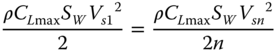
or

In terms of Imperial units, Eq. 17.8 becomes,
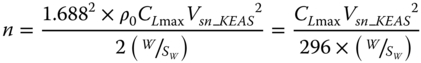
VA is the speed at which the positive stall and maximum load factor limits are simultaneously satisfied, that is, VA = VS1√nlimit.
The negative side of the boundary can be estimated in a similar fashion. For a cambered aerofoil, CLmax at a negative angle is less than at a positive angle.
VC is the design cruise speed. For a transport aircraft, VC must not be less than VB + 43 kt. The JARs contain more precise definitions plus definitions of several other speeds. In civil aviation, for an aircraft weight less than 50 000 lbs, the maximum manoeuvre load factor is usually +2.17. The appropriate expression to calculate the load factor is given by:
This is the required manoeuvre load factor at all speeds up to VC, unless the maximum achievable load factor is limited by stall.
Within the limit load, the negative value of n is −1.0 at speeds up to VC, decreasing linearly to 0 at VD (Figure 17.3). Maximum elevator deflection at VA and pitch rates from VA to VD must also be considered.
17.7.4 Manoeuvre Envelope Construction
Computational procedure:
- Assume V − KEAS and determine the flight Mach number.
- Apply the Mach number correction (experimental data, Figure 17.6) to revise the value of CLmax.
- Compute q = 0.50.5ρVsn2.
- Estimate n using Eq. 17.8 (Imperial units).
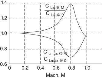
Figure 17.6 Effect of Mach number – experimental data [1].
17.7.5 High‐Speed Limit
VD is the maximum design speed. It is limited by the maximum dynamic pressure that the airframe can withstand. At high altitude, VD may be limited by the onset of high‐speed flutter.
17.8 Gust Envelope
Encountering unpredictable atmospheric disturbance is . Weather warnings help but full avoidance is not possible. Gusts can hit aircraft from any angle and the gust envelope can be shown in a separate set of diagrams. The most serious type is the vertical gust (Figure 17.3) affecting load factor n. Vertical gust increases the angle of attack, α, developing ΔL. Regulatory bodies have specified vertical gust rates that must be superimposed on the V‐n diagrams to describe limits of operation. It is standard practice to combine manoeuvre and gust envelope in one diagram as shown in Figures 17.2 and 17.5.
The FAR (14CFR) gives a detailed description to establish required gust loads. To keep within the ultimate load, the limits of vertical gust speeds are reduced with increase of aircraft speed. Pilots should fly at a lower speed if high turbulence is encountered. Examining Eq. 17.5, it can be seen that aircraft with low wing loading (W/SW), flying at high speeds are more affected by gust load. From statistical observations, the regulatory bodies (FAR (14CFR) Part 217.341a) have established maximum gust load at level flight as follows.
Linear interpolation is used to get appropriate velocities between 20 000 ft and 50 000 ft. Construction of V‐n diagrams is relatively easy from the aircraft specifications. The corner points of V‐n diagrams are specified. Computation to superimpose gust lines is more complex, for which FAR has given some semi‐empirical relations.
Flight speed, VB, is determined by the gust loads. It can be summarised as in Table 17.3.
VB is the design speed for maximum gust intensity. This definition assumes that the aircraft is in steady level flight at speed VB when it enters an idealised upward gust of air, which instantaneously increases the aircraft angle of attack and, hence, load factor. The increase in angle of attack must not stall the aircraft, that is, take it beyond the positive and negative stall boundaries.
Except in extreme weather conditions, this gust limit amounts to almost all‐weather flying. In gust, the aircraft load may cross the limit load but must not exceed ultimate load as shown in Figure 17.3. If the aircraft crosses the limit load, then appropriate action through inspection is carried out.
Given next is a brief outline to construct a V‐n diagram superimposed with gust load. The starting point for the gust envelope is when an aircraft is flying straight and level flight at n = 1. This is the starting point in developing the gust envelope. Actually, the gust reaches the aircraft in a velocity gradient and other aircraft characteristics; a factor is used to derive the gust load relationship [1]. A typical V‐n diagram with the gust speeds intersecting the lines is illustrated in Figures 17.4 and 17.7. The V‐n diagram is plotted with the x‐axis in VEAS. Separate V‐n diagrams are required for changes in aircraft weight and/or operating altitude.
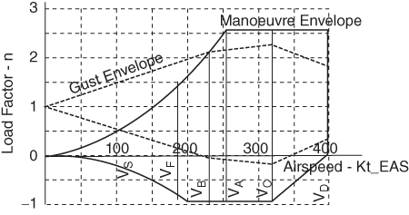
Figure 17.7 Composite V‐n diagram (typical of the Boeing707 type – courtesy of the Boeing Co. [2]) (A clean configuration at cruise speed and altitude).
17.8.1 Gust Load Equations
For a more extensive treatment, the readers may refer to Ref. [1]. The simplest way to consider gust load is to assume that a gust hits sharply in a sudden vertical velocity. Let UZ be the vertical velocity [1].
Increment of angle of attack Δα due to vertical velocity,
If V is in knots then Δα = UZ/(1.688 × V), UZ remains in ft s−1 and UZe is EAS in ft s−1.
(Note: UZ and V are in the same units, typically kept in EAS.)
Considerable simplification is made here to obtain satisfactory estimation. The simplification is made in establishing the value of CLα_aircraft (in brief CLα_ac). Typically, take CLα_aircraft to be 10% higher than CLα_wing. In this sub‐paragraph, CLα_aircraft is abbreviated to CLα_ac.
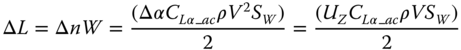
Incremental lift, ΔL, caused by the gust

Noting that VEAS = √σVTAS, Eq. 17.14a becomes
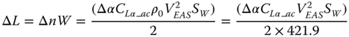
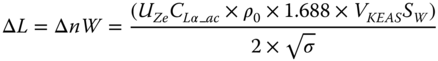
When VEAS is in knots, then this equation reduces to

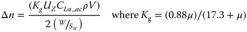
Modification to Eqs. (17.14a–c) is required as a vertical gust does not hit suddenly and sharply – it develops gradually. In addition to the gust gradient, other factors (the Kussner–Wagner effect) affecting the incremental load Δn are aircraft response characteristics (mass and geometry dependent) and lag in lift increments due to gradual increment of angle of attack Δα (aeroelastic effect). Incremental load Δn becomes less intense than compared to it encountering a sudden and sharp gust. An empirical factor Kg, known as ‘gust alleviation factor’ is applied and Eqs. (17.14a–c) becomes as follows.
Using Eq. 17.13 in Eq. 17.14a for Δα (velocities in ft s−1 true airspeed (TAS), i.e. UZ in ft s−1).
It becomes
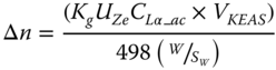
Eq. (17.14c), in KEAS becomes,

and where μ = 2W/(g × MAC × ρ × CLα_ac × SW)
When VEAS is in knots (VKEAS) then the Eq. reduces to
The higher the wing aspect ratio, the higher the CLα_ac and the higher the wing sweep, so the lower the CLα_ac. This means that a straight wing aircraft with a high wing aspect ratio will be more sensitive to loading than a swept wing with low aspect ratio. Military aircraft are more tolerant to gust load compared to turboprop drive civil transport aircraft.
Military aircraft requirements are slightly different from civil designs.
17.8.2 Gust Envelope Construction
Computational procedure
- Assume V − KEAS and determine the flight Mach number.
- Apply the Mach number correction (Figure 17.6) to revise the of CLmax and CLα.
- Compute q = 0.50.5ρVsn2.
- Estimate n using Eq. 17.11 (Imperial units).
Bizjet
Bizjet specification at sea level and 20 680 lb. Manoeuvre limit load = 3.0 to −1 and gust load limit = 4.5 to −1.17. The n range will increase at lighter weight and higher altitudes.
Maximum design cruising (level) speed VC at 20 000 ft altitude is the Mach 0.8 (TAS = 767.3 ft s−1, KEAS = 328.6). Maximum speed at dive is Mach 0.86 (380 KEAS).
To estimate manoeuvre load, n
FAR (14CFR) 217.337b gives n = 2.1 + 24 000/(W + 10 000) = 2.1 + 0.83 = 2.93.
Take n = 3.0 for the additional safety.
Negative manoeuvre load can be estimated in a similar manner.
Use Eq. 17.11,
In Imperial system,
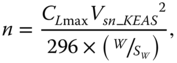
Use Figure 17.6 to correct CLmax (at low‐speed Mach number correction is not applied). To keep simple, the effect of relatively small amount of wing sweep on CLmax is ignored.
It gives,

Therefore, VA is at 180 KEAS to the limit of n = 3.0 (this is determined by plotting the locus of stall airspeed versus n).
To estimate gust load, ngust Eq. .
Incremental gust load Δn
NACA 65–410 given in Appendix F, take the lines for Re = 9 × 10⁶, as being close to the flight Reynolds number. It gives a 2D lift‐curve slope, dCl/dα = a0 = (1.05 – 0.25)/8 = 0.11/deg.
For a 3D wing,
is for the wing.
For an aircraft increase by 10%, that is,
Mach number correction (Figure 17.6) at 200 KEAS
or
and
Use Eq. (17.16a)

The readers may construct the full flight envelope (see the problem assignment in Appendix E).
References
- 1. Niu, M. (1999). Airframe Structural Design. Hong Kong: Commlit Press Ltd.
- 2. Boeing Document, Jet Aircraft Performance Methods (company usage) n.d..