57. Collision Detection

In a geometric context, collision detection refers to checking the relative configuration of two or more objects. The goal of collision detection, also known as interference detection or contact determination, is to automatically report a geometric contact when it is about to occur or has actually occurred. The objects may be represented as polygonal objects, spline or algebraic surfaces, deformable models, etc. Moreover, the objects may be static or dynamic.

Collision detection is a fundamental problem in computational geometry and frequently arises in different applications. These include:

1.Physically-based Modeling and Dynamic Simulation: The goal is to simulate dynamical systems and the physical behavior of objects subject to dynamic constraints. The mathematical model of the system is specified using geometric representations of the objects and the differential equations that govern the dynamics. The objects may undergo rigid or non-rigid motion. The contact interactions and trajectories of the objects are affected by collisions. It is important to model object interactions precisely and compute all the contacts accurately [1].

2.Motion Planning: The goal of motion planning is to compute a collision free path for a robot from a start configuration to a goal configuration. Motion planning is a fundamental problem in algorithmic robotics [2]. Most of the practical algorithms for motion planning compute different configurations of the robot and check whether these configurations are collision-free, that is, no collision between the robot and the objects in the environment. For example, probabilistic roadmap planners can spend up to 90% of the running time in collision checking.

3.Virtual Environments and Walkthroughs: A large-scale virtual environment, like a walkthrough, creates a computer-generated world, filled with real, simulated or virtual entities. Such an environment should give the user a feeling of presence, which includes making the images of both the user and the surrounding objects feel solid. For example, the objects should not pass through each other, and things should move as expected when pushed, pulled or grasped. Such actions require accurate and interactive collision detection. Moreover, runtime performance is critical in a virtual environment and all collision computations need to be performed at less than 1/30th of a second to give a sense of presence [3].

4.Haptic Rendering: Haptic interfaces, or force feedback devices, improve the quality of human-computer interaction by accommodating the sense of touch. In order to maintain a stable haptic system while displaying smooth and realistic forces and torques, haptic update rates must be as high as 1000 Hz. This involves accurately computing all contacts between the object attached to the probe and the simulated environment, as well as the restoring forces and torques—all in less than one millisecond [4].

In each of these applications, collision detection is one of the major computational bottlenecks.

Collision detection has been extensively studied in the literature for more than four decades. Hundreds of papers have been published on different aspects in computational geometry and related areas like robotics, computer graphics, virtual environments and computer-aided design. Most of the algorithms are designed to check whether a pair of objects collide. Some algorithms have been proposed for large environments composed of multiple objects and perform some form of culling or localize pairs of objects that are potentially colliding. At a broad level, different algorithms for collision detection can be classified based on the following characteristics:

•Query Type: The basic collision query checks whether two objects, described as set of points, polygons or other geometric primitives, overlap. This is the boolean form of the query. The enumerative version of the query yields some representations of the intersection set. Other queries compute the separation distance between two non-overlapping objects or the penetration distance between two overlapping objects.

•Object Types: Different algorithms have been proposed for convex polytopes, general polygonal models, curved objects described using parametric splines or implicit functions, set-theoretic combinations of objects, deformable models, etc.

•Motion Formulation: The collision query can be augmented by adding the element of time. If the trajectories of two objects are known, then we can determine when is the next time that a particular boolean query will become true or false. These queries are called dynamic queries, whereas the ones that do not use motion information are called static queries. In the case where the motion of an object can not be represented as a closed form function of time, the underlying application often performs static queries at specific time steps in the application.

In this chapter, we give a brief survey of different collision detection algorithms for convex polytopes, general polygonal models, penetration computations and large-scaled environments composed of multiple objects. In each category, we give a detailed description of one of the algorithms and the underlying data structures.

57.2Convex Polytopes

In this section, we give a brief survey of algorithms for collision detection between a pair of convex polytopes. This problem has been extensively studied and a number of algorithms with good asymptotic performance have been proposed. The best known runtime algorithm for boolean collision queries takes O(log2n) time, where n is the number of features [5]. It precomputes the Dobkin-Kirkpatrick hierarchy for each polytope and uses it to perform the runtime query. In practice, three classes of algorithms are commonly used for convex polytopes. These are linear programming, Minkowski sums, and tracking closest features based on Voronoi diagrams.

57.2.1Linear Programming

The problem of checking whether two convex polytopes intersect or not can be posed as a linear programming (LP) problem. In particular, two convex polytopes do not overlap, if and only if there exists a separation plane between them. The coefficients of the separation plane equation are treated as unknowns. The linear constraints are formulated by imposing that all the vertices of the first polytope lie in one half-space of this plane and those of the other polytope lie in the other half-space. The linear programming algorithms are used to check whether there is any feasible solution to the given set of constraints. Given the fixed dimension of the problem, some of the well-known linear programming algorithms [6] can be used to perform the boolean collision query in expected linear time.

57.2.2Voronoi-Based Marching Algorithm

An expected constant time algorithm for collision detection was proposed by Lin and Canny [7,8]. This algorithm tracks the closest features between two convex polytopes. The features may correspond to a vertex, an edge or a face of each polytope. Variants of this algorithm have also been presented in References 9,10. The original algorithm basically works by traversing the external Voronoi regions induced by the features of each convex polyhedron toward the pair of the closest features between the two given polytopes. The invariant is that at each step, either the inter-feature distance is reduced or the dimensionality of one or both of the features decreases by one, that is, a move from a face to an edge or from an edge to a vertex.

The algorithm terminates when the pair of testing features contain a pair of points that lie within the Voronoi regions of the other feature. It returns the pair of closest features and the Euclidean distance between them, as well as the contact status (i.e., colliding or not). This algorithm uses a modified boundary representation to represent convex polytopes and a data structure for describing “Voronoi regions” of convex polytopes.

57.2.2.1Polytope Representation

Let A be a polytope. A is partitioned into “features” $f_{1}, \dots, f_{n}$ $f_{1}, \dots, f_{n}$ where n is the total number of features, that is, n = f + e + v where f, e, v stands for the total number of faces, edges, vertices respectively. Each feature (except vertex) is an open subset of an affine plane and does not contain its boundary.

Definition: B is in the boundary of F and F is in coboundary of B, if and only if B is in the closure of F, that is, $B \subseteq \bar{F}$ $B \subseteq \bar{F}$ and B has one fewer dimension than F does.

For example, the coboundary of a vertex is the set of edges touching it and the coboundary of an edge are the two faces adjacent to it. The boundary of a face is the set of edges in the closure of the face. It uses winged edge representation, commonly used for boundary evaluation of boolean combinations of solid models [11]. The edge is oriented by giving two incident vertices (the head and tail). The edge points from tail to head. It has two adjacent faces cobounding it as well. Looking from the the tail end toward the head, the adjacent face lying to the right hand side is labeled as the “right face” and similarly for the “left face.”

Each polytope’s data structure has a field for its features (faces, edges, vertices) and Voronoi cells to be described below. Each feature is described by its geometric parameters. Its data structure also includes a list of its boundary, coboundary, and Voronoi regions.

Definition: A Voronoi region associated with a feature is a set of points exterior to the polyhedron which are closer to that feature than any other. The Voronoi regions form a partition of space outside the polyhedron according to the closest feature. The collection of Voronoi regions of each polyhedron is the generalized Voronoi diagram of the polyhedron. Note that the Voronoi diagram of a convex polyhedron has linear size and consists of polyhedral regions.

Definition: A Voronoi cell is the data structure for a Voronoi region. It has a set of constraint planes that bound its Voronoi region with pointers to the neighboring cells (each of which shares a common constraint plane with the given Voronoi cell) in its data structure.

Using the geometric properties of convex sets, “applicability criteria” are established based upon the Voronoi regions. That is, if a point P on object A lies inside the Voronoi region of f_B on object B, then f_B is a closest feature to the point P. If a point lies on a constraint plane, then it is equi-distant from the two features that share this constraint plane in their Voronoi cells.

57.2.2.2Local Walk

The algorithm incrementally traverses the features of each polytope to compute the closest features. For example, given a pair of features, Face 1 and vertex V_a on objects A and B, respectively, as the pair of initial features (Figure 57.1). The algorithm verifies if the vertex V_a lies within Cell 1 of Face 1. However, V_a violates the constraint plane imposed by CP of Cell 1, that is, V_a does not line in the half-space defined by CP which contains Cell 1. The constraint plane CP has a pointer to its adjacent cell Cell 2, so the walk proceeds to test whether V_a is contained within Cell 2. In similar fashion, vertex V_a has a cell of its own, and the algorithm checks whether the nearest point P_a on the edge to the vertex V_a lies within V_a’s Voronoi cell. Basically, the algorithm checks whether a point is contained within a Voronoi region defined by the constraint planes of the region. The constraint plane, which causes this test to fail, points to the next pair of closest features. Eventually, the algorithm computes the closest pair of features.

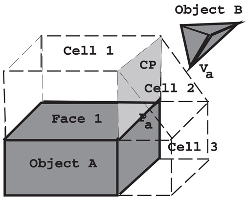
Figure 57.1A walk across Voronoi cells. Initially, the algorithm checks whether the vertex V_a lies in Cell 1. After it fails the containment test with respect to the plane CP, it walks to Cell 2 and checks for containment in Cell 2.

Since the polytopes and its faces are convex, the containment test involves only the neighboring features of the current candidate features. If either feature fails the test, the algorithm steps to a neighboring feature of one or both candidates, and tries again. With some simple preprocessing, the algorithm can guarantee that every feature of a polytope has a constant number of neighboring features. As a result, it takes a constant number of operations to check whether two features are the closest features.

This approach can be used in a static environment, but is especially well-suited for dynamic environments in which objects move in a sequence of small, discrete steps. The method takes advantage of coherence within two successive static queries: that is, the closest features change infrequently as the polytopes move along finely discretized paths. The closest features computed from the previous positions of the polytopes are used as the initial features for the current positions. The algorithm runs in expected constant time if the polytopes are not moving quickly. Even when a closest feature pair is changing rapidly, the algorithm takes only slightly longer. The running time is proportional to the number of feature pairs traversed, which is a function of the relative motion the polytopes undergo.

57.2.2.3Implementation and Application

The Lin-Canny algorithm has been implemented as part of several public-domain libraries, include I-COLLIDE and SWIFT [12]. It has been used for different applications including dynamic simulation [13], interactive walkthrough of architectural models [3] and haptic display (including force and torque computation) of polyhedral models [14].

57.2.3Minkowski Sums and Convex Optimization

The collision and distance queries can be performed based on the Minkowski sum of two objects. Given two sets of points, P and Q, their Minkowski sum is the set of points:

{p + q | p \in P, q \in Q .}

${p + q | p \in P, q \in Q .}$

It has been shown in Reference 15, that the minimum separation distance between two objects is the same as the minimum distance from the origin of the Minkowski sums of A and − B to the surface of the sums. The Minkowski sum is also referred to as the translational C-space obstacle (TCSO) If we take the TCSO of two convex polyhedra, A and B, then the TCSO is another convex polyhedra, and each vertex of the TCSO correspond to the vector difference of a vertex from A and a vertex from B. While the Minkowski sum of two convex polytopes can have O(n2) features [16], a fast algorithm for separation distance computation based on convex optimization that exhibits linear-time performance in practice has been proposed by Gilbert et al. [17]. It is also known as the GJK algorithm. It uses pairs of vertices from each object that define simplices (i.e., a point, bounded line, triangle or tetrahedron) within each polyhedra and a corresponding simplex in the TCSO. Initially the simplex is set randomly and the algorithm refines it using local optimization, till it computes the closest point on the TCSO from the origin of the Minkowski sums. The algorithm assumes that the origin is not inside the TCSO.

By taking the similar philosophy as the Lin-Canny algorithm [8], Cameron [18] presented an extension to the basic GJK algorithm by exploiting motion coherence and geometric locality in terms of connectivity between neighboring features. It keeps track of the witness points, a pair of points from the two objects that realize the minimum separation distance between them. As opposed to starting from a random simplex in the TCSO, the algorithm starts with the witness points from the previous iteration and performs hill climbing to compute a new set of witness points for the current configuration. The running time of this algorithm is a function of the number of refinement steps that the algorithm has to perform.

57.3General Polygonal Models

Algorithms for collision and separation distance queries between general polygons models can be classified based on the fact whether they are closed polyhedral models or represented as a collection of polygons. The latter, also referred to as “polygon soups,” make no assumption related to the connectivity among different faces or whether they represent a closed set.

Some of the commonly known algorithms for collision detection and separation distance computation use spatial partitioning or bounding volume hierarchies (BVHs). The spatial subdivisions are a recursive partitioning of the embedding space, whereas bounding volume hierarchies are based on a recursive partitioning of the primitives of an object. These algorithms are based on the divide-and-conquer paradigm. Examples of spatial partitioning hierarchies include k-D trees and octrees [19], R-trees and their variants [20], cone trees, BSPs [21] and their extensions to multi-space partitions [22]. The BVHs use bounding volumes (BVs) to bound or contain sets of geometric primitives, such as triangles, polygons, curved surfaces, etc. In a BVH, BVs are stored at the internal nodes of a tree structure. The root BV contains all the primitives of a model, and children BVs each contain separate partitions of the primitives enclosed by the parent. Each of the leaf node BVs typically contains one primitive. In some variations, one may place several primitives at a leaf node, or use several volumes to contain a single primitive. The BVHs are used to perform collision and separation distance queries. These include sphere-trees [23,24], AABB-trees [20,25, 26], OBB-trees [27–29], spherical shell-trees [30,31], k-DOP-trees [32,33], SSV-trees [34], and convex hull-trees [35]. Different BVHs can be classified based on:

•Choice of BV: The AABB-tree uses an axis-aligned bounding box (AABB) as the underlying BV. The AABB for a set of primitives can be easily computed from the extremal points along the X, Y and Z direction. The sphere tree uses a sphere as the underlying BV. Algorithms to compute a minimal bounding sphere for a set of points in 3D are well known in computational geometry. The k-DOP-tree is an extension of the AABB-tree, where each BV is computed from extremal points along k fixed directions, as opposed to the 3 orthogonal axes. A spherical shell is a subset of the volume contained between two concentric spheres and is a tight fitting BV. A SSV (swept sphere volume) is defined by taking the Minkowski sum of a point, line or a rectangle in 3D with a sphere. The SSV-tree corresponds to a hybrid hierarchy, where the BVs may correspond to a point-swept sphere (PSS), a line-swept sphere (LSS) or a rectangle-swept sphere (RSS). Finally, the BV in the convex-hull tree is a convex polytope.

•Hierarchy generation: Most of the algorithms for building hierarchies fall into two categories: bottom-up and top-down. Bottom-up methods begin with a BV for each primitive and merge volumes into larger volumes until the tree is complete. Top-down methods begin with a group of all primitive, and recursively subdivide until all leaf nodes are indivisible. In practice, top-down algorithms are easier to implement and typically take $O (n \lg n)$ $O (n \lg n)$ time, where n is the number of primitives. On the other hand, the bottom-up methods use clustering techniques to group the primitives at each level and can lead to tighter-fitting hierarchies.

The collision detection queries are performed by traversing the BVHs. Two models are compared by recursively traversing their BVHs in tandem. Each recursive step tests whether BVs A and B, one from each hierarchy, overlap. If A and B do not overlap, the recursion branch is terminated. But if A and B overlap, the enclosed primitives may overlap and the algorithm is applied recursively to their children. If A and B are both leaf nodes, the primitives within them are compared directly. The running time of the algorithm is dominated by the overlap tests between two BVs and a BV and a primitive. It is relatively simple to check whether two AABBs overlap or two spheres overlap or two k-DOPs overlap. Specialized algorithms have also been proposed to check whether two OBBs, two SSVs, two spherical shells or two convex polytopes overlap. Next, we described a commonly used interference detection algorithm that uses hierarchies of oriented bounding boxes.

57.3.1Interference Detection Using Trees of Oriented Bounding Boxes

In this section we describe an algorithm for building a BVH of OBBs (called OBBTree) and using them to perform fast interference queries between polygonal models. More details about the algorithm are available in References 27,29.

The underlying algorithm is applicable to all triangulated models. They need not represent a compact set or have a manifold boundary representation. As part of a preprocess, the algorithm computes a hierarchy of oriented bounding boxes (OBBs) for each object. At runtime, it traverses the hierarchies to check whether the primitives overlap.

57.3.1.1OBBTree Construction

An OBBTree is a bounding volume tree of OBBs. Given a collection of triangles, the algorithm initially approximates them with an OBB of similar dimensions and orientation. Next, it computes a hierarchy of OBBs.

The OBB computation algorithm makes use of first and second order statistics summarizing the vertex coordinates. They are the mean, μ, and the covariance matrix, C, respectively [36]. If the vertices of the i’th triangle are the points pi, qi, and ri, then the mean and covariance matrix can be expressed in vector notation as:

μ = \frac{1}{3 n} \sum_{i = 0}^{n} (p^{i} + q^{i} + r^{i}),

$μ = \frac{1}{3 n} \sum_{i = 0}^{n} (p^{i} + q^{i} + r^{i}),$

C_{j k} = \frac{1}{3 n} \sum_{i = 0}^{n} ({\bar{p}}_{j}^{i} {\bar{p}}_{k}^{i} + {\bar{q}}_{j}^{i} {\bar{q}}_{k}^{i} + {\bar{r}}_{j}^{i} {\bar{r}}_{k}^{i}), 1 \leq j, k \leq 3

$C_{j k} = \frac{1}{3 n} \sum_{i = 0}^{n} ({\bar{p}}_{j}^{i} {\bar{p}}_{k}^{i} + {\bar{q}}_{j}^{i} {\bar{q}}_{k}^{i} + {\bar{r}}_{j}^{i} {\bar{r}}_{k}^{i}), 1 \leq j, k \leq 3$

where n is the number of triangles, ${\bar{p}}^{i} = p^{i} - μ$ ${\bar{p}}^{i} = p^{i} - μ$ , ${\bar{q}}^{i} = q^{i} - μ$ ${\bar{q}}^{i} = q^{i} - μ$ , and ${\bar{r}}^{i} = r^{i} - μ$ ${\bar{r}}^{i} = r^{i} - μ$ . Each of them is a 3 × 1 vector, for example, ${\bar{p}}^{i} = ({\bar{p}}_{1}^{i}, {\bar{p}}_{2}^{i}, {\bar{p}}_{3}^{i})^{T}$ ${\bar{p}}^{i} = ({\bar{p}}_{1}^{i}, {\bar{p}}_{2}^{i}, {\bar{p}}_{3}^{i})^{T}$ and C_jk are the elements of the 3 by 3 covariance matrix.

The eigenvectors of a symmetric matrix, such as C, are mutually orthogonal. After normalizing them, they are used as a basis. The algorithm finds the extremal vertices along each axis of this basis. Two of the three eigenvectors of the covariance matrix are the axes of maximum and of minimum variance, so they will tend to align the box with the geometry of a tube or a flat surface patch.

The algorithm’s performance can be improved by using the convex hull of the vertices of the triangles. To get a better fit, we can sample the surface of the convex hull densely, taking the mean and covariance of the sample points. The uniform sampling of the convex hull surface normalizes for triangle size and distribution.

One can sample the convex hull “infinitely densely” by integrating over the surface of each triangle, and allowing each differential patch to contribute to the covariance matrix. The resulting integral has a closed form solution. Let the area of the i’th triangle in the convex hull be denoted by

A^{i} = \frac{1}{2} | (p^{i} - q^{i}) \times (p^{i} - r^{i}) |

$A^{i} = \frac{1}{2} | (p^{i} - q^{i}) \times (p^{i} - r^{i}) |$

Let the surface area of the entire convex hull be denoted by

A^{H} = \sum_{i} A^{i}

$A^{H} = \sum_{i} A^{i}$

Let the centroid of the i’th convex hull triangle be denoted by

c^{i} = (p^{i} + q^{i} + r^{i}) / 3

$c^{i} = (p^{i} + q^{i} + r^{i}) / 3$

Let the centroid of the convex hull, which is a weighted average of the triangle centroids (the weights are the areas of the triangles), be denoted by

c^{H} = \frac{\sum_{i} A^{i} c^{i}}{\sum_{i} A^{i}} = \frac{\sum_{i} A^{i} c^{i}}{A^{H}}

$c^{H} = \frac{\sum_{i} A^{i} c^{i}}{\sum_{i} A^{i}} = \frac{\sum_{i} A^{i} c^{i}}{A^{H}}$

The elements of the covariance matrix C have the following closed-form,

C_{j k} = \sum_{i = 1}^{n} \frac{A^{i}}{12 A^{H}} (9 c_{j}^{i} c_{k}^{i} + p_{j}^{i} p_{k}^{i} + q_{j}^{i} q_{k}^{i} + r_{j}^{i} r_{k}^{i}) - c_{j}^{H} c_{k}^{H}

$C_{j k} = \sum_{i = 1}^{n} \frac{A^{i}}{12 A^{H}} (9 c_{j}^{i} c_{k}^{i} + p_{j}^{i} p_{k}^{i} + q_{j}^{i} q_{k}^{i} + r_{j}^{i} r_{k}^{i}) - c_{j}^{H} c_{k}^{H}$

Given an algorithm to compute tight-fitting OBBs around a group of polygons, we need to represent them hierarchically. The simplest algorithm for OBBTree computation uses a top-down method. It is based on a subdivision rule that splits the longest axis of a box with a plane orthogonal to one of its axes, partitioning the polygons according to which side of the plane their center point lies on (a 2-D analog is shown in Figure 57.2). The subdivision coordinate along that axis is chosen to be that of the mean point, μ, of the vertices. If the longest axis cannot not be subdivided, the second longest axis is chosen. Otherwise, the shortest one is used. If the group of polygons cannot be partitioned along any axis by this criterion, then the group is considered indivisible.

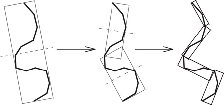
Figure 57.2Building the OBBTree: recursively partition the bounded polygons and bound the resulting groups. This figure shows three levels of an OBBTree of a polygonal chain.

Given a model with n triangles, the overall time to build the tree is $O (n \log^{2} n)$ $O (n \log^{2} n)$ if we use convex hulls, and $O (n \log n)$ $O (n \log n)$ if we don’t. The recursion is similar to that of quicksort. Fitting a box to a group of n triangles and partitioning them into two subgroups takes $O (n \log n)$ $O (n \log n)$ with a convex hull and O(n) without it. Applying the process recursively creates a tree with leaf nodes $O (\log n)$ $O (\log n)$ levels deep.

57.3.1.2Interference Detection

Given OBBTrees of two objects, the interference algorithm typically spends most of its time testing pairs of OBBs for overlap. The algorithm computes axial projections of the bounding boxes and check for disjointness along those axes. Under this projection, each box forms an interval on the axis (a line in 3D). If the intervals don’t overlap, then the axis is called a ‘separating axis’ for the boxes, and the boxes must then be disjoint.

It has been shown that we need to perform at most 15 axial projections in 3D to check whether two OBBs overlap or not [29]. These 15 directions correspond to the face normals of each OBB, as well as 9 pairwise combinations obtained by taking the cross-product of the vectors representing their edges.

To perform the test, the algorithm projects the centers of the boxes onto the axis, and also to compute the radii of the intervals. If the distance between the box centers as projected onto the axis is greater than the sum of the radii, then the intervals (and the boxes as well) are disjoint. This is shown in 2D in Figure 57.3.

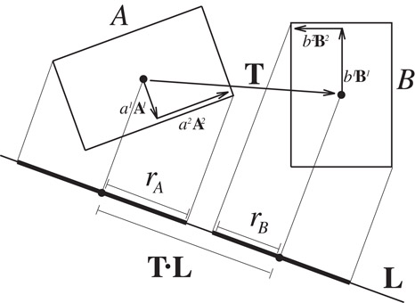
Figure 57.3 $\vec{L}$ $\vec{L}$ is a separating axis for OBBs A and B because A and B become disjoint intervals under projection (shown as r_A and r_B, respectively) onto $\vec{L}$ $\vec{L}$ .

57.3.1.3OBB Representation and Overlap Test

We assume we are given two OBBs, A and B, with B placed relative to A by rotation matrix $\vec{R}$ $\vec{R}$ and translation vector $\vec{T}$ $\vec{T}$ . The half-dimensions (or “radii’) of A and B are a_i and b_i, where i = 1, 2, 3. We will denote the axes of A and B as the unit vectors ${\vec{A}}^{i}$ ${\vec{A}}^{i}$ and ${\vec{B}}^{i}$ ${\vec{B}}^{i}$ , for i = 1, 2, 3. These will be referred to as the 6 box axes. Note that if we use the box axes of A as a basis, then the three columns of $\vec{R}$ $\vec{R}$ are the same as the three ${\vec{B}}^{i}$ ${\vec{B}}^{i}$ vectors.

The centers of each box projects onto the midpoint of its interval. By projecting the box radii onto the axis, and summing the length of their images, we obtain the radius of the interval. If the axis is parallel to the unit vector $\vec{L}$ $\vec{L}$ , then the radius of box A’s interval is

r_{A} = \sum_{i} | a_{i} {\vec{A}}^{i} \cdot \vec{L} |

$r_{A} = \sum_{i} | a_{i} {\vec{A}}^{i} \cdot \vec{L} |$

A similar expression is used to compute r_B.

The placement of the axis is immaterial, so we assume it passes through the center of box A. The distance between the midpoints of the intervals is $| \vec{T} \cdot \vec{L} |$ $| \vec{T} \cdot \vec{L} |$ . So, the intervals are disjoint if and only if

| \vec{T} \cdot \vec{L} | > \sum_{i} | a_{i} {\vec{A}}^{i} \cdot \vec{L} | + \sum_{i} | b_{i} {\vec{B}}^{i} \cdot \vec{L} |

$| \vec{T} \cdot \vec{L} | > \sum_{i} | a_{i} {\vec{A}}^{i} \cdot \vec{L} | + \sum_{i} | b_{i} {\vec{B}}^{i} \cdot \vec{L} |$

This simplifies when $\vec{L}$ $\vec{L}$ is a box axis or cross product of box axes. For example, consider $\vec{L} = {\vec{A}}^{1} \times {\vec{B}}^{2}$ $\vec{L} = {\vec{A}}^{1} \times {\vec{B}}^{2}$ . The second term in the first summation is

\begin{aligned} | a_{2} {\vec{A}}^{2} \cdot ({\vec{A}}^{1} \times {\vec{B}}^{2}) | & = | a_{2} {\vec{B}}^{2} \cdot ({\vec{A}}^{2} \times {\vec{A}}^{1}) | \\ = | a_{2} {\vec{B}}^{2} \cdot {\vec{A}}^{3} | \\ = | a_{2} {\vec{B}}_{3}^{2} | \\ = a_{2} | {\vec{R}}_{32} | \end{aligned}

$\begin{aligned} | a_{2} {\vec{A}}^{2} \cdot ({\vec{A}}^{1} \times {\vec{B}}^{2}) | & = | a_{2} {\vec{B}}^{2} \cdot ({\vec{A}}^{2} \times {\vec{A}}^{1}) | \\ = | a_{2} {\vec{B}}^{2} \cdot {\vec{A}}^{3} | \\ = | a_{2} {\vec{B}}_{3}^{2} | \\ = a_{2} | {\vec{R}}_{32} | \end{aligned}$

The last step is due to the fact that the columns of the rotation matrix are also the axes of the frame of B. The original term consisted of a dot product and cross product, but reduced to a multiplication and an absolute value. Some terms reduce to zero and are eliminated. After simplifying all the terms, this axis test looks like:

| {\vec{T}}_{3} {\vec{R}}_{22} - {\vec{T}}_{2} {\vec{R}}_{32} | > a_{2} | {\vec{R}}_{32} | + a_{3} | {\vec{R}}_{22} | + b_{1} | {\vec{R}}_{13} | + b_{3} | {\vec{R}}_{11} |

$| {\vec{T}}_{3} {\vec{R}}_{22} - {\vec{T}}_{2} {\vec{R}}_{32} | > a_{2} | {\vec{R}}_{32} | + a_{3} | {\vec{R}}_{22} | + b_{1} | {\vec{R}}_{13} | + b_{3} | {\vec{R}}_{11} |$

All 15 axis tests simplify in similar fashion. Among all the tests, the absolute value of each element of $\vec{R}$ $\vec{R}$ is used four times, so those expressions can be computed once before beginning the axis tests. If any one of the expressions is satisfied, the boxes are known to be disjoint, and the remainder of the 15 axis tests are unnecessary. This permits early exit from the series of tests. In practice, it takes up to 200 arithmetic operations in the worst case to check whether two OBBs overlap.

57.3.1.4Implementation and Application

The OBBTree interference detection algorithm has been implemented and used as part of the following packages: RAPID, V-COLLIDE and PQP [12]. These implementations have been used for robot motion planning, dynamic simulation and virtual prototyping.

57.3.2Performance of Bounding Volume Hierarchies

The performance of BVHs on proximity queries is governed by a number of design parameters. These include techniques to build the trees, number of children each node can have, and the choice of BV type. An additional design choice is the descent rule. This is the policy for generating recursive calls when a comparison of two BVs does not prune the recursion branch. For instance, if BVs A and B failed to prune, one may recursively compare A with each of the children of B, B with each of the children of A, or each of the children of A with each the children of B. This choice does not affect the correctness of the algorithm, but may impact the performance. Some of the commonly used algorithms assume that the BVHs are binary trees and each primitive is a single triangle or a polygon. The cost of performing the collision query is given as [27,34]:

T = N_{b v} \times C_{b v} + N_{p} \times C_{p},

$T = N_{b v} \times C_{b v} + N_{p} \times C_{p},$

where T is the total cost function for collision queries, N_bv is the number of bounding volume pair operations, and C_bv is the total cost of a BV pair operation, including the cost of transforming and updating (including resizing) each BV for use in a given configuration of the models, and other per BV-operation overhead. N_p is the number of primitive pairs tested for proximity, and C_p is the cost of testing a pair of primitives for proximity (e.g., overlaps or distance computation).

Typically for tight fitting bounding volumes, for example, oriented bounding boxes (OBBs), N_bv and N_p are relatively low, whereas C_bv is relatively high. In contrast, C_bv is low while N_bv and N_p may be higher for simple BV types like spheres and axis-aligned bounding boxes (AABBs). Due to these opposing trends, no single BV yields optimum performance for collision detection in all possible cases.

57.4Penetration Depth Computation

In this section, we give a brief overview of penetration depth (PD) computation algorithms between convex polytopes and general polyhedral models. The PD of two inter-penetrating objects A and B is defined as the minimum translation distance that one object undergoes to make the interiors of A and B disjoint. It can be also defined in terms of the TCSO. When two objects are overlapping, the origin of the Minkowski sum of A and −B is contained inside the TCSO. The penetration depth corresponds to the minimum distance from the origin to the surface of TCSO [18]. PD computation is often used in motion planning [37], contact resolution for dynamic simulation [38,39] and force computation in haptic rendering [40]. For example, computation of dynamic response in penalty-based methods often needs to perform PD queries for imposing the non-penetration constraint for rigid body simulation. In addition, many applications, such as motion planning and dynamic simulation, require a continuous distance measure when two (non-convex) objects collide, in order to have a well-posed computation.

Some of the algorithms for PD computation involve computing the Minkowski sums and computing the closest point on its surface from the origin. The worst case complexity of the overall PD algorithm is governed by the complexity of computing Minkowski sums, which can be O(n2) for convex polytopes and O(n6) for general (or non-convex) polyhedral models [16]. Given the complexity of Minkowski sums, many approximation algorithms have been proposed in the literature for fast PD estimation.

57.4.1Convex Polytopes

Dobkin et al. [16] have proposed a hierarchical algorithm to compute the directional PD using Dobkin and Kirkpatrick polyhedral hierarchy. For any direction d, it computes the directional penetration depth in O(log n log m) time for polytopes with m and n vertices. Agarwal et al. [41] have presented a randomized approach to compute the PD values [41]. It runs in $O (m^{\frac{3}{4} + ϵ} n^{\frac{3}{4} + ϵ} + m^{1 + ϵ} + n^{1 + ϵ})$ $O (m^{\frac{3}{4} + ϵ} n^{\frac{3}{4} + ϵ} + m^{1 + ϵ} + n^{1 + ϵ})$ expected time for any positive constant ε. Cameron [18] has presented an extension to the GJK algorithm [17] to compute upper and lower bounds on the PD between convex polytopes. Bergen has further elaborated this idea in an expanding polytope algorithm [42]. The algorithm iteratively improves the result of the PD computation by expanding a polyhedral approximation of the Minkowski sums of two polytopes.

57.4.2Incremental Penetration Depth Computation

Kim et al. [43] have presented an incremental penetration depth (PD) algorithm that marches towards a “locally optimal” solution by walking on the surface of the Minkowski sum. The surface of the TCSO is implicitly computed by constructing a local Gauss map and performing a local walk on the polytopes.

This algorithm uses the concept of width computation from computational geometry. Given a set of points $P = {p_{1}, p_{2}, \dots, p_{n}}$ $P = {p_{1}, p_{2}, \dots, p_{n}}$ in 3D, the width of P, W(P), is defined as the minimum distance between parallel planes supporting P. The width W(P) of convex polytopes A and B is closely related to the penetration depth PD(A, B), since it is easy to show that W(P) = PD(P, P). It can be shown that width and penetration depth computation can be reduced to searching only the VF and EE antipodal pairs (where V, E and F denote a vertex, edge and face, respectively, of the polytopes). This is accomplished by using the standard dual mapping on the Gauss map (or normal diagram). The mapping is defined from object space to the surface of a unit sphere $S^{2}$ $S^{2}$ as: a vertex is mapped to a region, a face to a point, and an edge to a great arc. The algorithm finds the antipodal pairs by overlaying the upper hemisphere of the Gauss map on the lower hemisphere and computing the intersections between them.

57.4.2.1Local Walk

The incremental PD computation algorithm does not compute the entire Gauss map for each polytope or the entire boundary of the Minkowski sum. Rather it computes them in a lazy manner based on local walking and optimization. Starting from some feature on the surface of the Minkowski sum, the algorithm computes the direction in which it can decrease the PD value and proceeds towards that direction by extending the surface of the Minkowski sum.

At each iteration of the algorithm, a vertex is chosen from each polytope to form a pair. It is called a vertex hub pair and the algorithm uses it as a hub for the expansion of the local Minkowski sum. The vertex hub pair is chosen in such a way that there exists a plane supporting each polytope, and is incident on each vertex. It turns out that the vertex hub pair corresponds to two intersected convex regions on a Gauss map, which later become intersecting convex polygons on the plane after central projection. The intersection of convex polygons corresponds to the VF or EE antipodal pairs that are used to reconstruct the local surface of the Minkowski sum around the vertex hub pair. Given these pairs, the algorithm chooses the one that corresponds to the shortest distance from the origin of the Minkowski sum to their surface. If this pair decreases the estimated PD value, the algorithm updates the current vertex hub pair to the new adjacent pair. This procedure is repeated until the algorithm can not decrease the current PD value and converges to a local minima.

57.4.2.2Initialization and Refinement

The algorithm starts with an initial guess on the vertex hub pair. A good estimate to the penetration direction can be obtained by taking the centroid difference between the objects, and computing an extremal vertex pair for the difference direction. In other cases, the penetrating features (for overlapping polytopes) or the closest features (from non-overlapping polytopes) from the previous instance can also suggest a good initial guess.

After the algorithm obtains a initial guess for a VV pair, it iteratively seeks to improve the PD estimate by jumping from one VV pair to an adjacent VV pair. This is accomplished by looking around the neighborhood of the current VV pair and walking to a pair which provides the greatest improvement in the PD value. Let the current vertex hub pair be v1v′₁. The next vertex hub pair v2v′₂ is computed as follows:

1.Construct a local Gauss map each for v1 and v′₁,

2.Project the Gauss maps onto z = 1 plane, and label them as G and G′, respectively. G and G′ correspond to convex polygons in 2D.

3.Compute the intersection between G and G′ using a linear time algorithm such as [44]. The result is a convex polygon and let u_i be a vertex of the intersection set. If u_i is an original vertex of G or G′, it corresponds to the VF antipodal pair in object space. Otherwise, it corresponds to an EE antipodal pair.

4.In object space, determine which u_i corresponds to the best local improvement in PD, and set an adjacent vertex pair (adjacent to u_i) to v2v′₂.

This iteration is repeated until either there is no more improvement in the PD value or number of iterations reach some maximum value. At step 4 of the iteration, the next vertex hub pair is selected in the following manner. If u_i corresponds to VF, then the algorithm chooses one of the two vertices adjacent to F assuming that the model is triangulated. The same reasoning is also applied to when u_i corresponds to EE. As a result, the algorithm needs to perform one more iteration in order to actually decide which vertex hub pair should be selected. A snapshot of a typical step during the iteration is illustrated in Figure 57.4. Eventually the algorithm computes a local minima.

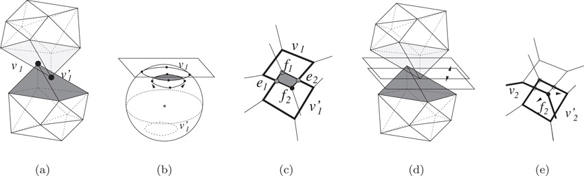
Figure 57.4Iterative optimization for incremental PD computation: (a) The current VV pair is v1v′₁ and a shaded region represents edges and faces incident to v1v′₁. (b) shows local Gauss maps and their overlay for v1v′₁. (c) shows the result of the overlay after central projection onto a plane. Here, f1, e1, f2 and e2 comprise vertices (candidate PD features) of the overlay. (d) illustrates how to compute the PD for the candidate PD features in object space. (e) f2 is chosen as the next PD feature, thus v2v′₂ is determined as the next vertex hub pair.

57.4.2.3Implementation and Application

The incremental algorithm is implemented as part of DEEP [12]. It works quite well in practice and is also able to compute the global penetration depth in most cases. It has been used for 6-DOF haptic rendering (force and torque display), dynamic simulation and virtual prototyping.

57.4.3Non-Convex Models

Algorithms for penetration depth estimation between general polygonal models are based on discretization of the object space containing the objects or use of digital geometric algorithms that perform computations on a finite resolution grid. Fisher and Lin [45] have presented a PD estimation algorithm based on the distance field computation using the fast marching level-set method. It is applicable to all polyhedral objects as well as deformable models, and it can also check for self-penetration. Hoff et al. [46,47] have proposed an approach based on performing discretized computations on the graphics rasterization hardware. It uses multi-pass rendering techniques for different proximity queries between general rigid and deformable models, including penetration depth estimation. Kim et al. [43] have presented a fast approximation algorithm for general polyhedral models using a combination of object-space as well discretized computations. Given the global nature of the PD problem, it decomposes the boundary of each polyhedron into convex pieces, computes the pairwise Minkowski sums of the resulting convex polytopes and uses graphics rasterization hardware to perform the closest point query up to a given discretized resolution. The results obtained are refined using a local walking algorithm. To further speed up this computation and improve the estimate, the algorithm uses a hierarchical refinement technique that takes advantage of geometry culling, model simplification, accelerated ray-shooting, and local refinement with greedy walking. The overall approach combines discretized closest point queries with geometry culling and refinement at each level of the hierarchy. Its accuracy can vary as a function of the discretization error. It has been applied to haptic rendering and dynamic simulation.

57.5Large Environments

Large environments are composed of multiple moving objects. Different methods have been proposed to overcome the computational bottleneck of O(n2) pairwise tests in an environment composed of n objects. The problem of performing proximity queries in large environments, is typically divided into two parts [3,23]: the broad phase, in which we identify the pair of objects on which we need to perform different proximity queries, and the narrow phase, in which we perform the exact pairwise queries. In this section, we present a brief overview of algorithms used in the broad phase.

The simplest algorithms for large environments are based on spatial subdivisions. The space is divided into cells of equal volume, and at each instance the objects are assigned to one or more cells. Collisions are checked between all object pairs belonging to each cell. In fact, Overmars has presented an efficient algorithm based on hash table to efficient perform point location queries in fat subdivisions [48]. This approach works well for sparse environments in which the objects are uniformly distributed through the space. Another approach operates directly on four-dimensional volumes swept out by object motion over time [49].

57.5.1Multiple-Object Collision Detection

Large-scale environments consist of stationary as well as moving objects. Let there be N moving objects and M stationary objects. Each of the N moving objects can collide with the other moving objects, as well as with the stationary ones. Keeping track of (N2) + NM pairs of objects at every time step can become time consuming as N and M get large. To achieve interactive rates, we must reduce this number before performing pairwise collision tests. In this section, we give an overview of sweep-and-prune algorithm used to perform multiple-object collision detection [3]. The overall architecture of the multiple object collision detection algorithm is shown in Figure 57.5.

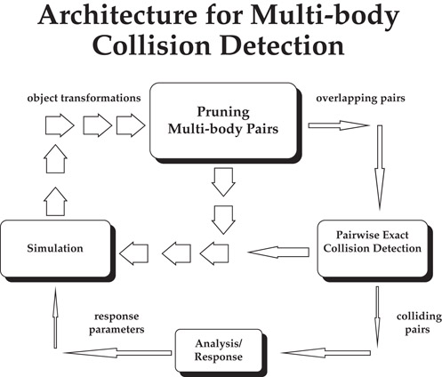
Figure 57.5Architecture for multiple body collision detection algorithm.

The algorithm uses sorting to prune the number of pairs. Each object is surrounded by a 3-dimensional bounding volume. These bounding volumes are sorted in 3-space to determine which pairs are overlapping. The algorithm only needs to perform exact pairwise collision tests on these remaining pairs.

However, it is not intuitively obvious how to sort objects in 3-space. The algorithm uses a dimension reduction approach. If two bodies collide in a 3-dimensional space, their orthogonal projections onto the xy, yz, and xz-planes and x, y, and z-axes must overlap. Based on this observation, the algorithm uses axis-aligned bounding boxes and efficiently project them onto a lower dimension, and perform sorting on these lower-dimensional structures.

The algorithm computes a rectangular bounding box to be the tightest axis-aligned box containing each object at a particular orientation. It is defined by its minimum and maximum x, y, and z-coordinates. As an object moves, the algorithm recomputes its minima and maxima, taking into account the object’s orientation.

As a precomputation, the algorithm computes each object’s initial minima and maxima along each axis. It is assumed that the objects are convex. For non-convex polyhedral models, the following algorithm is applied to their convex hulls. As an object moves, its minima and maxima are recomputed in the following manner:

1.Check to see if the current minimum (or maximum) vertex for the x, y, or z-coordinate still has the smallest (or largest) value in comparison to its neighboring vertices. If so the algorithm terminates.

2.Update the vertex for that extreme direction by replacing it with the neighboring vertex with the smallest (or largest) value of all neighboring vertices. Repeat the entire process as necessary.

This algorithm recomputes the bounding boxes at an expected constant rate. It exploits the temporal and geometric coherence.

The algorithm does not transform all the vertices as the objects undergo motion. As it is updating the bounding boxes, new positions are computed for current vertices using matrix-vector multiplications. This approach is optimized based on the fact that the algorithm is interested in one coordinate value of each extremal vertex, say the x coordinate while updating the minimum or maximum value along the x-axis. Therefore, there is no need to transform the other coordinates in order to compare neighboring vertices. This reduces the number of arithmetic operations by two-thirds, as we only compute a dot-product of two vectors and do not perform matrix-vector multiplication.

57.5.1.1One-Dimensional Sweep and Prune

The one-dimensional sweep and prune algorithm begins by projecting each three-dimensional bounding box onto the x, y, and z axes. Because the bounding boxes are axis-aligned, projecting them onto the coordinate axes results in intervals (see Figure 57.6). The goal is to compute the overlaps among these intervals, because a pair of bounding boxes can overlap if and only if their intervals overlap in all three dimensions.

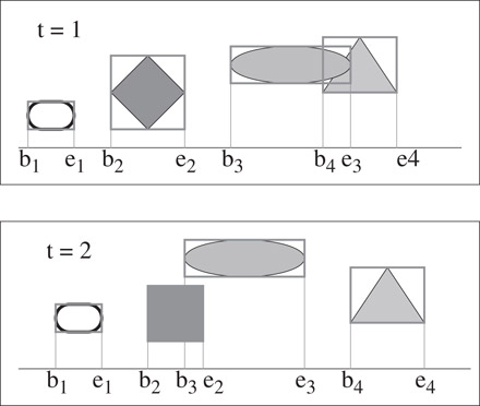
Figure 57.6Bounding box behavior between successive instances. Notice the coherence between the 1D list obtained after projection onto the X-axis.

The algorithm constructs three lists, one for each dimension. Each list contains the values of the endpoints of the intervals corresponding to that dimension. By sorting these lists, it determines which intervals overlap. In the general case, such a sort would take O(n log n) time, where n is the number of objects. This time bound is reduced by keeping the sorted lists from the previous frame, changing only the values of the interval endpoints. In environments where the objects make relatively small movements between frames, the lists will be nearly sorted, so we can sort in expected O(n) time, as shown in References 50,51. In practice, insertion sort works well for almost sorted lists.

In addition to sorting, the algorithm keeps track of changes in the overlap status of interval pairs (i.e., from overlapping in the last time step to non-overlapping in the current time step, and vice-versa). This can be done in O(n + e_x + e_y + e_z) time, where e_x, e_y, and e_z are the number of exchanges along the x, y, and z-axes. This also runs in expected linear time due to coherence, but in the worst case e_x, e_y, and e_z can each be O(n2) with an extremely small constant.

This algorithm is suitable for dynamic environments where coherence between successive static queries is preserved. In computational geometry literature several algorithms exist that solve the static version of determining 3-D bounding box overlaps in O(n log2n + s) time, where s is the number of pairwise overlaps [52,53]. It has been reduced to to O(n + s) by exploiting coherence.

57.5.1.2Implementation and Application

The sweep-and-prune has been used in some of the widely uses collision detection systems, including I-COLLIDE, V-COLLIDE, SWIFT and SWIFT++ [12]. It has been used for multi-body simulations and interactive walkthroughs of complex environments.

57.5.2Two-Dimensional Intersection Tests

The two-dimensional intersection algorithm begins by projecting each three-dimensional axis-aligned bounding box onto any two of the x-y, x-z, and y-z planes. Each of these projections is a rectangle in 2-space. Typically there are fewer overlaps of these 2-D rectangles than of the 1-D intervals used by the sweep and prune technique. This results in fewer swaps as the objects move. In situations where the projections onto one-dimension result in densely clustered intervals, the two-dimensional technique is more efficient. The interval tree is a common data structure for performing such two-dimensional range queries [54].

Each query of an interval intersection takes O(log n + k) time where k is the number of reported intersections and n is the number of intervals. Therefore, reporting intersections among n rectangles can be done in O(n log n + K) where K is the total number of intersecting rectangles [55].

References

1.D. Baraff and A. Witkin, Physically-Based Modeling: ACM SIGGRAPH Course Notes, 2001.

2.J. Latombe, Robot Motion Planning. Kluwer Academic Publishers, Boston, MA, 1991.

3.J. Cohen, M. Lin, D. Manocha, and M. Ponamgi. I-collide: An interactive and exact collision detection system for large-scale environments. Proc. of ACM Interactive 3D Graphics Conference, pp. 189–196, 1995.

4.M. A. Otaduy, and M. C. Lin. Sensation preserving simplification for haptic rendering. Proc. of ACM SIGGRAPH, 2003.

5.D. P. Dobkin and D. G. Kirkpatrick, Determining the separation of preprocessed polyhedra—a unified approach, in Proc. 17th Internat. Colloq. Automata Lang. Program., vol. 443 of Lecture Notes in Computer Science, pp. 400–413, Springer-Verlag, 1990.

6.R. Seidel, Linear programming and convex hulls made easy, Proc. 6th Ann. ACM Conf. on Computational Geometry, (Berkeley, California), pp. 211–215, 1990.

7.M. Lin, Efficient Collision Detection for Animation and Robotics: PhD thesis, Department of Electrical Engineering and Computer Science, University of California, Berkeley, December 1993.

8.M. Lin, and J. F. Canny, Efficient algorithms for incremental distance computation. IEEE Conference on Robotics and Automation, pp. 1008–1014, 1991.

9.S. Ehmann, and M. C. Lin, Accelerated proximity queries between convex polyhedra using multi-level voronoi marching. Proc. of IEEE/RSJ International Conference on Intelligent Robots and Systems, pp. 2101–2106, 2000.

10.B. Mirtich, V-Clip: Fast and robust polyhedral collision detection, ACM Transactions on Graphics, vol. 17, pp. 177–208, July 1998.

11.C. Hoffmann, Geometric and Solid Modeling. San Mateo, California: Morgan Kaufmann, 1989.

12.Collision detection systems. http://gamma.web.unc.edu/software/#collision, 2002.

13.B. Mirtich and J. Canny, Impulse-based simulation of rigid bodies, Proc. of ACM Interactive 3D Graphics, (Monterey, CA), 1995.

14.A. Gregory, A. Mascarenhas, S. Ehmann, M. C. Lin, and D. Manocha, 6-dof haptic display of polygonal models. Proc. of IEEE Visualization Conference, 2000.

15.S. Cameron, and R. K. Culley, Determining the minimum translational distance between two convex polyhedra. Proceedings of International Conference on Robotics and Automation, pp. 591–596, 1986.

16.D. Dobkin, J. Hershberger, D. Kirkpatrick, and S. Suri, Computing the intersection-depth of polyhedra, Algorithmica, vol. 9, pp. 518–533, 1993.

17.E. G. Gilbert, D. W. Johnson, and S. S. Keerthi, A fast procedure for computing the distance between objects in three-dimensional space, IEEE J. Robotics and Automation, vol. RA-4, pp. 193–203, 1988.

18.S. Cameron. Enhancing GJK: Computing minimum and penetration distance between convex polyhedra. Proceedings of International Conference on Robotics and Automation, pp. 3112–3117, 1997.

19.H. Samet, Spatial Data Structures: Quadtree, Octrees and Other Hierarchical Methods. Addison Wesley, Reading, MA, 1989.

20.M. Held, J. Klosowski, and J. Mitchell. Evaluation of collision detection methods for virtual reality fly-throughs. Canadian Conference on Computational Geometry, 1995.

21.B. Naylor, J. Amanatides, and W. Thibault. Merging bsp trees yield polyhedral modeling results. Proc. of ACM SIGGRAPH, pp. 115–124, 1990.

22.W. Bouma, and G. Vanecek. Collision detection and analysis in a physically based simulation. Proceedings Eurographics Workshop on Animation and Simulation, pp. 191–203, 1991.

23.P. M. Hubbard, Interactive collision detection, Proceedings of IEEE Symposium on Research Frontiers in Virtual Reality, October 1993.

24.S. Quinlan. Efficient distance computation between non-convex objects. Proceedings of International Conference on Robotics and Automation, pp. 3324–3329, 1994.

25.N. Beckmann, H. Kriegel, R. Schneider, and B. Seeger, The r*-tree: An efficient and robust access method for points and rectangles. Proc: SIGMOD Conf. on Management of Data, pp. 322–331, 1990.

26.M. Ponamgi, D. Manocha, and M. Lin, Incremental algorithms for collision detection between solid models, IEEE Transactions on Visualization and Computer Graphics, vol. 3, no. 1, pp. 51–67, 1997.

27.S. Gottschalk, M. Lin, and D. Manocha. OBB-Tree: A hierarchical structure for rapid interference detection. Proc. of ACM Siggraph’96, pp. 171–180, 1996.

28.G. Barequet, B. Chazelle, L. Guibas, J. Mitchell, and A. Tal, Boxtree: A hierarchical representation of surfaces in 3D. Proc. of Eurographics’96, 1996.

29.S. Gottschalk, Collision Queries using Oriented Bounding Boxes: PhD thesis, University of North Carolina. Department of Computer Science, 2000.

30.S. Krishnan, A. Pattekar, M. Lin, and D. Manocha. Spherical shell: A higher order bounding volume for fast proximity queries. Proc. of Third International Workshop on Algorithmic Foundations of Robotics, pp. 122–136, 1998.

31.S. Krishnan, M. Gopi, M. Lin, D. Manocha, and A. Pattekar, Rapid and accurate contact determination between spline models using shelltrees, Computer Graphics Forum, Proceedings of Eurographics, vol. 17, no. 3, pp. C315–C326, 1998.

32.M. Held, J. Klosowski, and J. S. B. Mitchell, Real-time collision detection for motion simulation within complex environments, in Proc. ACM SIGGRAPH’96 Visual Proceedings, p. 151, 1996.

33.J. Klosowski, M. Held, J. Mitchell, H. Sowizral, and K. Zikan, Efficient collision detection using bounding volume hierarchies of k-dops, IEEE Trans. on Visualization and Computer Graphics, vol. 4, no. 1, pp. 21–37, 1998.

34.E. Larsen, S. Gottschalk, M. Lin, and D. Manocha, Fast proximity queries with swept sphere volumes,” Tech. Rep. TR99-018, Department of Computer Science, University of North Carolina, 1999. 32 pages.

35.S. Ehmann and M. C. Lin, Accurate and fast proximity queries between polyhedra using convex surface decomposition, Computer Graphics Forum (Proc. of Eurographics’2001), vol. 20, no. 3, pp. 500–510, 2001.

36.R. Duda and P. Hart, Pattern Classification and Scene Analysis. John Wiley and Sons, 1973.

37.D. Hsu, L. Kavraki, J. Latombe, R. Motwani, and S. Sorkin. On finding narrow passages with probabilistic roadmap planners. Proc. of 3rd Workshop on Algorithmic Foundations of Robotics, pp. 25–32, 1998.

38.M. McKenna and D. Zeltzer, Dynamic simulation of autonomous legged locomotion, Computer Graphics (SIGGRAPH ’90 Proceedings) (F. Baskett, ed.), vol. 24, pp. 29–38, Aug. 1990.

39.D. E. Stewart and J. C. Trinkle, An implicit time-stepping scheme for rigid body dynamics with inelastic collisions and coulomb friction, International Journal of Numerical Methods in Engineering, vol. 39, pp. 2673–2691, 1996.

40.Y. Kim, M. Otaduy, M. Lin, and D. Manocha. 6-dof haptic display using localized contact computations. Proc. of Haptics Symposium, pp. 209–216, 2002.

41.P. Agarwal, L. Guibas, S. Har-Peled, A. Rabinovitch, and M. Sharir, Penetration depth of two convex polytopes in 3d, Nordic J: Computing, vol. 7, pp. 227–240, 2000.

42.G. Bergen. Proximity queries and penetration depth computation on 3d game objects. Game Developers Conference, 2001.

43.Y. Kim, M. Lin, and D. Manocha. Deep: An incremental algorithm for penetration depth computation between convex polytopes. Proc. of IEEE Conference on Robotics and Automation, pp. 921–926, 2002.

44.J. O’Rourke, C.-B. Chien, T. Olson, and D. Naddor A new linear algorithm for intersecting convex polygons, Comput. Graph. Image Process., vol. 19, pp. 384–391, 1982.

45.S. Fisher, and M. C. Lin. Deformed distance fields for simulation of non-penetrating flexible bodies. Proc. of EG Workshop on Computer Animation and Simulation, pp. 99–111, 2001.

46.K. Hoff, A. Zaferakis, M. Lin, and D. Manocha. Fast and simple 2d geometric proximity queries using graphics hardware. Proc. of ACM Symposium on Interactive 3D Graphics, pp. 145–148, 2001.

47.K. Hoff, A. Zaferakis, M. Lin, and D. Manocha, Fast 3d geometric proximity queries between rigid and deformable models using graphics hardware acceleration, Tech. Rep. TR02-004, Department of Computer Science, University of North Carolina, 2002.

48.M. H. Overmars, Point location in fat subdivisions, Inform. Proc. Lett., vol. 44, pp. 261–265, 1992.

49.S. Cameron. Collision detection by four-dimensional intersection testing. Proceedings of International Conference on Robotics and Automation, pp. 291–302, 1990.

50.D. Baraff, Dynamic simulation of non-penetrating rigid body simulation. PhD thesis, Cornell University, 1992.

51.M. Shamos, and D. Hoey, Geometric intersection problems. Proc. 17th An. IEEE Symp. Found. on Comput. Science, pp. 208–215, 1976.

52.J. Hopcroft, J. Schwartz, and M. Sharir, Efficient detection of intersections among spheres, The International Journal of Robotics Research, vol. 2, no. 4, pp. 77–80, 1983.

53.H. Six, and D. Wood, Counting and reporting intersections of D-ranges. IEEE Transactions on Computers, pp. 46–55, 1982.

54.F. Preparata and M. I. Shamos, Computational Geometry. New York: Springer-Verlag, 1985.

55.H. Edelsbrunner, A new approach to rectangle intersections, Part I, Internat. J. Comput. Math., vol. 13, pp. 209–219, 1983.

^⋆This chapter has been reprinted from first edition of this Handbook, without any content updates.

..................Content has been hidden....................

You can't read the all page of ebook, please click here login for view all page.

Table of Contents for 57. Collision Detection

Create new playlist

Sign In

Sign Up

Table of Contents for
57. Collision Detection