19. Interval, Segment, Range, Priority Search Trees

In this chapter, we introduce four basic data structures that are of fundamental importance and have many applications as we will briefly cover them in later sections. They are interval trees, segment trees, range trees, and priority search trees. Consider for example the following problems. Suppose we have a set of iso-oriented rectangles in the plane. A set of rectangles are said to be iso-oriented if their edges are parallel to the coordinate axes. The subset of iso-oriented rectangles defines a clique, if their common intersection is nonempty. The largest subset of rectangles whose common intersection is non-empty is called a maximum clique. The problem of finding this largest subset with a non-empty common intersection is referred to as the maximum clique problem for a rectangle intersection graph [1,2].^* The k-dimensional, k ≥ 1, analog of this problem is defined similarly. In one-dimensional (1D) case, we will have a set of intervals on the real line, and an interval intersection graph, or simply interval graph. The maximum clique problem for interval graphs is to find a largest subset of intervals whose common intersection is non-empty. The cardinality of the maximum clique is sometimes referred to as the density of the set of intervals.

The problem of finding a subset of objects that satisfy a certain property is often referred to as the searching problem. For instance, given a set of numbers S = {x1, x2, …, x_n}, where x_i ∈ ℜ, i = 1, 2, …, n, the problem of finding the subset of numbers that lie between a range [ℓ, r], that is, F = {x ∈ S|ℓ ≤ x ≤ r}, is called an (1D) range search problem [3,4].

To deal with this kind of geometric searching problem, we need to have appropriate data structures to support efficient searching algorithms. The data structure is assumed to be static, that is, the input set of objects is given a priori, and no insertions or deletions of the objects are allowed. If the searching problem satisfies decomposability property, that is, if they are decomposable,^† then there are general dynamization schemes available [7], that can be used to convert static data structures into dynamic ones, where insertions and deletions of objects are permitted. Examples of decomposable searching problems include the membership problem in which one queries if a point p lies in S. Let S be partitioned into two subsets S1 and S2, and Member(p, S) returns yes, if p ∈ S, and no otherwise. It is easy to see that Member(p, S)= OR(Member(p, S1), Member(p, S2)), where OR is a Boolean operator.

19.2Interval Trees

Consider a set S of intervals, S = {I_i|i = 1, 2, …, n}, each of which is specified by an ordered pair, I_i = [ℓ_i, r_i], ℓ_i, r_i ∈ ℜ, ℓ_i ≤ r_i, i = 1, 2, …, n.

An interval tree [8,9], Interval_Tree(S), for S is a rooted augmented binary search tree, in which each node v has a key value, v.key, two tree pointers v.left and v.right to the left and right subtrees, respectively, and an auxiliary pointer, v.aux to an augmented data structure, and is recursively defined as follows:

•The root node v associated with the set S, denoted Interval_Tree_root(S), has key value v.key equal to the median of the 2 × |S| endpoints. This key value v.key divides S into three subsets S_ℓ, S_r, and S_m, consisting of sets of intervals lying totally to the left of v.key, lying totally to the right of v.key, and containing v.key, respectively. That is, Sℓ={Ii|ri<v.key} $S_{ℓ} = {I_{i} | r_{i} < v . k e y}$ , S_r = {I_j|v.key < ℓ_j}, and S_m = {I_k|ℓ_k ≤ v.key ≤ r_k}.

•Tree pointer v.left points to the left subtree rooted at Interval_Tree_root(S_ℓ), and tree pointer v.right points to the right subtree rooted at Interval_Tree_root(S_r).

•Auxiliary pointer v.aux points to an augmented data structure consisting of two sorted arrays, SA(S_m.left) and SA(S_m.right) of the set of left endpoints of the intervals in S_m and the set of right endpoints of the intervals in S_m, respectively. That is, S_m.left = {ℓ_i|I_i ∈ S_m} and S_m.right = {r_i|I_i ∈ S_m}.

19.2.1Construction of Interval Trees

The following is a pseudo code for the recursive construction of the interval tree of a set S of n intervals. Without loss of generality, we shall assume that the endpoints of these n intervals are all distinct. See Figure 19.1a for an illustration.

function Interval_Tree(S)

/* It returns a pointer v to the root, Interval_Tree_root(S), of the interval tree for a set S of intervals. */

Input: A set S of n intervals, S = {I_i|i = 1, 2, …, n} and each interval I_i = [ℓ_i, r_i], where ℓ_i and r_i are the left and right endpoints, respectively of I_i, ℓ_i, r_i ∈ ℜ, and ℓ_i ≤ r_i, i = 1, 2, …, n.

Output: An interval tree, rooted at Interval_Tree_root(S).

Method:

1.if S = ∅ return nil.

2.Create a node v such that v.key equals x, where x is the middle point of the set of endpoints so that there are exactly |S|/2 endpoints less than or equal to x and greater than x, respectively. Let Sℓ={Ii|ri<x} $S_{ℓ} = {I_{i} | r_{i} < x}$ , S_r = {I_j|x < ℓ_j}, and S_m = {I_k|ℓ_k ≤ x ≤ r_k}.

3.Set v.left equal to Interval_Tree(S_ℓ).

4.Set v.right equal to Interval_Tree(S_r).

5.Create a node w which is the root node of an auxiliary data structure associated with the set S_m of intervals, such that w.left and w.right point to two sorted arrays, SA(S_m.left) and SA(S_m.right), respectively. SA(S_m.left) denotes an array of left endpoints of intervals in S_m in ascending order, and SA(S_m.right) an array of right endpoints of intervals in S_m in descending order.

6.Set v.aux equal to node w.

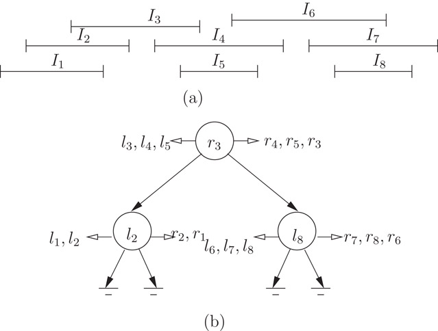
Figure 19.1Interval tree for S = {I1, I2, …, I8} and its interval models.

Note that this recursively built interval tree structure requires O(n) space, where n is the cardinality of S, since each interval is either in the left subtree, the right subtree, or the middle augmented data structure.

19.2.2Example and Its Applications

Figure 19.1b illustrates an example of an interval tree of a set of intervals, spread out as shown in Figure 19.1a.

The interval trees can be used to handle quickly queries of the following forms.

Enclosing Interval Searching Problem [10,11]: Given a set S of n intervals and a query point q, report all those intervals containing q, that is, find a subset F ⊆ S such that F = {I_i|ℓ_i ≤ q ≤ r_i}.

Overlapping Interval Searching Problem [8,9,12]: Given a set S of n intervals and a query interval Q, report all those intervals in S overlapping Q, that is, find a subset F ⊆ S such that F = {I_i|I_i ∩ Q ≠ ∅}.

The following pseudo code solves the Overlapping Interval Searching Problem in O(log n) + |F| time. It is invoked by a call to Overlapping_Interval_Search(v, Q, F), where v is Interval_Tree_root(S), and F, initially set to be ∅, will contain the set of intervals overlapping query interval Q.

procedure Overlapping_Interval_Search(v, Q, F)

Output: A subset F = {I_i | I_i ∩ Q ≠ ∅}.

Method:

1.Set F = ∅ initially.

2.if v is nil return.

3.if (v.key ∈ Q) then

for each interval I_i in the augmented data structure pointed to by v.aux

do F = F ∪ {I_i}.

Overlapping_Interval_Search(v.left, Q, F)

Overlapping_Interval_Search(v.right, Q, F)

4.if (r < v.key) then

for each left endpoint ℓ_i in the sorted array pointed to by v.aux.left such that ℓ_i < r

do F = F ∪ {I_i}.

Overlapping_Interval_Search(v.left, Q, F)

5.if (ℓ > v.key) then

for each right endpoint r_i in the sorted array pointed to by v.aux.right such that r_i > ℓ

do F = F ∪ {I_i}.

Overlapping_Interval_Search(v.right, Q, F)

It is obvious to see that an interval I in S overlaps a query interval Q = [ℓ, r] if (i) Q contains the left endpoint of I, (ii) Q contains the right endpoint of I, or (iii) Q is totally contained in I. Step 3 reports those intervals I that contain a point v.key which is also contained in Q. The for-loop of Step 4 reports intervals in either case (i) or (iii) and the for-loop of Step 5 reports intervals in either case (ii) or (iii).

Note the special case of procedure Overlapping_Interval_Search(v, Q, F) when we set the query interval Q = [ℓ, r] so that its left and right endpoints coincide, that is, ℓ = r will report all the intervals in S containing a query point, solving the Enclosing Interval Searching Problem.

However, if one is interested in the problem of finding a special type of overlapping intervals, for example, all intervals containing or contained in a given query interval [10,11], the interval tree data structure does not necessarily yield an efficient solution. Similarly, the interval tree does not provide an effective method to handle queries about the set of intervals, for example, the maximum clique, or the measure, the total length of the union of the intervals [13,14].

We conclude with the following theorem.

Theorem 19.1

The Enclosing Interval Searching Problem and Overlapping Interval Searching Problem for a set S of n intervals can both be solved in O(log n) time (plus time for output) and in linear space.

19.3Segment Trees

The segment tree structure, originally introduced by Bentley [3,4], is a data structure for intervals whose endpoints are fixed or known a priori. The set S = {I1, I2, …, I_n} of n intervals, each of which is represented by I_i = [ℓ_i, r_i], ℓ_i, r_i ∈ ℜ, ℓ_i ≤ r_i, is represented by a data array, Data_Array(S), whose entries correspond to the endpoints, ℓ_i or r_i, and are sorted in non-decreasing order. This sorted array is denoted SA[1…N], N = 2n. That is, SA[1] ≤ SA[2] ≤ ··· ≤ SA[N]. We will in this section use the indexes in the range [1, N] to refer to the entries in the sorted array SA[1…N]. For convenience, we will be working in the transformed domain using indexes, and a comparison involving a point q ∈ ℜ and an index i ∈ ℵ, unless otherwise specified, is performed in the original domain in ℜ. For instance, q < i is interpreted as q < SA[i].

The segment tree structure, as will be demonstrated later, can be useful in finding the measure of a set of intervals. That is, the length of the union of a set of intervals. It can also be used to find the maximum clique of a set of intervals. This structure can be generalized to higher dimensions.

19.3.1Construction of Segment Trees

The segment tree, as the interval tree discussed in Section 19.2 is a rooted augmented binary search tree, in which each node v is associated with a range of integers v.range = [v.B, v.E], v.B, v.E ∈ ℵ, v.B < v.E, representing a range of indexes from v.B to v.E, a key v.key that splits v.range into two subranges, each of which is associated with each child of v, two tree pointers v.left and v.right to the left and right subtrees, respectively, and an auxiliary pointer, v.aux to an augmented data structure. Given integers s and t, with 1 ≤ s < t ≤ N, the segment tree, denoted Segment_Tree(s, t), is recursively described as follows:

•The root node v, denoted Segment_Tree_root(s, t), is associated with the range [s, t], and v.B = s and v.E = t.

•If s + 1 = t, then we have a leaf node v with v.B = s, v.E = t, and v.key = nil.

•Otherwise (i.e., s + 1 < t), let m be the mid-point of s and t, or m = ⌊(v.B + v.E)/2⌋. Set v.key = m.

•Tree pointer v.left points to the left subtree rooted at Segment_Tree_root(s, m), and tree pointer v.right points to the right subtree rooted at Segment_Tree_root(m, t).

•Auxiliary pointer v.aux points to an augmented data structure, associated with the range [s, t], whose content depends on the usage of the segment tree.

The following is a pseudo code for the construction of a segment tree for a range [s, t] s < t, s, t ∈ ℵ, and the construction of a set of n intervals whose endpoints are indexed by an array of integers in the range [1, N], N = 2n can be done by a call to Segment_Tree(1, N). See Figure 19.2b for an illustration.

function Segment_Tree(s, t)

/* It returns a pointer v to the root, Segment_Tree_root(s, t), of the segment tree for the range [s, t].*/

Input: A set N $N$ of integers, {s, s + 1, …, t} representing the indexes of the endpoints of a subset of intervals.

Output: A segment tree, rooted at Segment_Tree_root(s, t).

Method:

1.Let v be a node, v.B = s, v.E = t, v.left = v.right = nil, and v.aux to be determined.

2.if s + 1 = t then return.

3.Let v.key = m = ⌊(v.B + v.E)/2⌋.

4.v.left = Segment_Tree(s, m)

5.v.right = Segment_Tree(m, t)

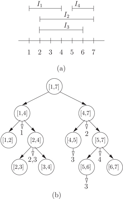
Figure 19.2Segment tree of S = {I1, I2, I3, I4} and its interval models.

The parameters v.B and v.E associated with node v define a range [v.B, v.E], called a standard range associated with v. The standard range associated with a leaf node is also called an elementary range. It is straightforward to see that Segment_Tree(s, t) constructed in function Segment_Tree(s, t) described above is balanced, and has height, denoted Segment_Tree(s, t).height, equal to ⌈ log2(t − s)⌉.

We now introduce the notion of canonical covering of a range [b, e], where b, e ∈ ℵ and 1 ≤ b < e ≤ N. A node v in Segment_Tree(1, N) is said to be in the canonical covering of [b, e] if its associated standard range satisfies this property [v.B, v.E] ⊆ [b, e], while that of its parent node does not. It is obvious that if a node v is in the canonical covering, then its sibling node, that is, the node with the same parent node as the present one, is not, for otherwise the common parent node would have been in the canonical covering. Thus, at each level, there are at most two nodes that belong to the canonical covering of [b, e].

Thus, for each range [b, e], the number of nodes in its canonical covering is at most ⌈ log2(e − b)⌉ + ⌊ log2(e − b)⌋ − 2. In other words, a range [b, e] (or respectively an interval [b, e]) can be decomposed into at most ⌈ log2(e − b)⌉ + ⌊ log2(e − b)⌋ − 2 standard ranges (or respectively subintervals) [3,4].

To identify the nodes in a segment tree T that are in the canonical covering of an interval I = [b, e], representing a range [b, e], we perform a call to Interval_Insertion(v, b, e, Q), where v is Segment_Tree_root(1, N). The procedure Interval_Insertion(v, b, e, Q) is defined below.

procedure Interval_Insertion(v, b, e, Q)

/* It returns a queue Q of nodes q ∈ T such that [v.B, v.E] ⊆ [b, e] but [u.B,u.E]⊊[b,e] $[u . B, u . E] ⊊ [b, e]$ , where u is the parent node of v. */

Input: A segment tree T pointed to by its root node, v = Segment_Tree_root(1, N), for a set S of intervals.

Output: A queue Q of nodes in T that are in the canonical covering of [b, e].

Method:

1.Initialize an output queue Q, which supports insertion (⇒Q) and deletion (⇐Q) in constant time.

2.if ([v.B, v.E] ⊆ [b, e]) then append [b, e] to v, v ⇒ Q and return.

3.if (b < v.key) then Interval_Insertion(v.left, b, e, Q)

4.if (v.key < e) then Interval_Insertion(v.right, b, e, Q)

To append [b, e] to a node v means to insert interval I = [b, e] into the auxiliary structure associated with node v to indicate that node v whose standard range is totally contained in I is in the canonical covering of I. If the auxiliary structure v.aux associated with node v is an array, the operation append [b, e] to a node v can be implemented as v.aux[j++] = I.

procedure Interval_Insertion(v, b, e, Q) described above can be used to represent a set S of n intervals in a segment tree by performing the insertion operation n times, one for each interval. As each interval I can have at most O(log n) nodes in its canonical covering, and hence we perform at most O(log n) append operations for each insertion, the total amount of space required in the auxiliary data structures reflecting all the nodes in the canonical covering is O(n log n).

Deletion of an interval represented by a range [b, e] can be done similarly, except that the append operation will be replaced by its corresponding inverse operation remove that removes the interval from the auxiliary structure associated with some canonical covering node.

Theorem 19.2

The segment tree for a set S of n intervals can be constructed in O(n log n) time, and if the auxiliary structure for each node v contains a list of intervals containing v in the canonical covering, then the space required is O(n log n).

To simplify the description, given a set S of intervals, we assume that the endpoints of the intervals are represented by the indexes of a sorted array SA[1 N], N = 2|S|, containing these endpoints, and the segment tree representing this set is abbreviated as Segment_Tree(S) in the remaining of this section.

19.3.2Examples and Its Applications

Figure 19.2b illustrates an example of a segment tree of the set of intervals, as shown in Figure 19.2a. The integers, if any, under each node v represent the indexes of intervals that contain the node in its canonical covering. For example, Interval I2 contains nodes labeled by standard ranges [2,4] and [4,7].

We now describe how segment trees can be used to solve the Enclosing Interval Searching Problem defined before, the Maximum Clique Problem of a set of intervals, and that of a set of rectangles, which are defined below.

Maximum Clique Size of a set of Intervals [2,15,16]: Given a set S = {I1, I2, …, I_n} of n intervals, a clique is a subset C_I ⊆ S such that the common intersection of intervals in C_I is non-empty, and a maximum clique is a clique of maximum size. That is, ⋂Ii∈CI⊆SIi≠∅ $⋂_{I_{i} \in C_{I} \subseteq S} I_{i} \neq \emptyset$ and |C_I| is maximized. The problem is to find the maximum size |C_I|.

Maximum Clique Size of a set of Rectangles [2]: Given a set S = {R1, R2, …, R_n} of n rectangles, a clique is a subset C_R ⊆ S such that the common intersection of rectangles in C_R is non-empty, and a maximum clique is a clique of maximum size. That is, ⋂Ri∈CR⊆SRi≠∅ $⋂_{R_{i} \in C_{R} \subseteq S} R_{i} \neq \emptyset$ and |C_R| is maximized. The problem is to find the maximum size |C_R|.

The following pseudo code solves the Enclosing Interval Searching Problem in O(log n) + |F| time, where F is the output set. It is invoked by a call Point_in_Interval_Search(v, q, F), where v is Segment_Tree_root(S), and F, initially set to be ∅, will contain the set of intervals containing a query point q.

procedure Point_in_Interval_Search(v, q, F)

/* It returns in F the list of intervals stored in the segment tree pointed to by v and containing query point q. */

Input: A segment tree representing a set S of n intervals, S = {I_i|i = 1, 2, …, n} and a query point q ∈ ℜ. The auxiliary structure v.aux associated with each node v is a list of intervals I ∈ S that contain v in their canonical coverings.

Output: A subset F = {I_i|ℓ_i ≤ q ≤ r_i}.

Method:

1.if v is nil or (q < v.B or q > v.E) then return.

2.if (v.B ≤ q ≤ v.E) then

for each interval I_i in the auxiliary data structure pointed to by v.aux do F = F ∪ {I_i}.

3.if (q ≤ v.key) then Point_in_Interval_Search(v.left, q, F)

4.else (/* i.e., q > v.key */) Point_in_Interval_Search(v.right, q, F)

We now address the problem of finding the size of the maximum clique of a set S of intervals, S = {I1, I2, …, I_n}, where each interval I_i = [ℓ_i, r_i], and ℓ_i ≤ r_i, ℓ_i, r_i ∈ ℜ, i = 1, 2, …, n. There are other approaches, such as plane-sweep [2,4,15,16], that solve this problem within the same complexity.

For this problem, we introduce an auxiliary data structure to be stored at each node v. v.aux will contain two pieces of information: one is the number of intervals containing v in the canonical covering, denoted v.♯, and the other is the clique size, denoted v.clq. The clique size of a node v is the size of the maximum clique whose common intersection is contained in but not equal to the standard range associated with v. It is defined to be equal to the larger of the two numbers: v.left.♯ + v.left.clq and v.right.♯ + v.right.clq. For a leaf node v, v.clq = 0. The size of the maximum clique for the set of intervals will then be stored at the root node r = Segment_Tree_root(S) and is equal to the sum of r.♯ and r.clq. It is obvious that the space needed for this segment tree is linear.

As this data structure supports insertion of intervals incrementally, it can be used to answer the maximum clique of the current set of intervals as the intervals are inserted into (or deleted from) the segment tree T. The following pseudo code finds the size of the maximum clique of a set of intervals.

function Interval_Maximum_Clique_Size(S)

/* It returns the size of the maximum clique of a set S of intervals. */

Input: A set S of n intervals and the segment tree T rooted at r = Segment_Tree_root(S).

Output: An integer, which is the size of the maximum clique of S.

Method:

1.Initialize v.clq = v.♯ = 0 for all nodes v in T.

2.for each interval I_i = [ℓ_i, r_i] ∈ S, i = 1, 2, …, n do

/* Insert I_i into the tree and update v.♯ and v.clq for all visited nodes and those nodes in the canonical covering of I_i. */

clq_S_i = Update_Segment_Tree_by_Weight(r, ℓ_i, r_i, +1) (see below).

3.return clq_S_n.

function Update_Segment_Tree_by_Weight(v, b, e, w)

/* Insert into/delete from the segment tree pointed to by v the interval I = [b, e] and update v.♯ and v.clq by w for all visited nodes and those nodes in the canonical covering of I. */

Input: A segment tree rooted at v containing a set of intervals, an interval I = [b, e] to be inserted/deleted, b, e ∈ ℜ, b ≤ e, and a weight w ∈ {+1, −1}, where +1 corresponds to insertion and −1 to deletion.

Output: An integer, which is the size of the maximum clique of the set of intervals after update.

Method:

1.if ([v.B, v.E] ⊆ [b, e]) then

v.♯ = v.♯ + w

return v.♯ + v.clq

2.if (b < v.key) then Update_Segment_Tree_by_Weight(v.left, b, e, w)

3.if (v.key < e) then Update_Segment_Tree_by_Weight(v.right, b, e, w)

4.v.clq=max{v.left.♯+v.left.clq,v.right.♯+v.right.clq} $v . c l q = max {v . left . ♯ + v . left . c l q, v . right . ♯ + v . right . c l q}$

5.return v.♯ + v.clq

Note that function Update_Segment_Tree_by_Weight(v, b, e, w) visits at most O(log n) nodes in the canonical covering of I and takes O(log n) time. Since function Interval_Maximum_Clique_Size(S) invokes the function n times, we obtain the following theorem.

Theorem 19.3

Given a set S = {I1, I2, …, I_n} of n intervals, the size of the maximum clique of S_i = {I1, I2, …, I_i} can be found in O(i log n) time and linear space, for each i = 1, 2, …, n, by using a segment tree.

Next, we extend the study of the maximum clique size problem to its 2D version, finding the size of the maximum clique of a set S of rectangles, S = {R1, R2, …, R_n}, where each rectangle Ri=[xℓ,i,xr,i]×[yℓ,i,yr,i] $R_{i} = [x_{ℓ, i}, x_{r, i}] \times [y_{ℓ, i}, y_{r, i}]$ , xℓ,i,xr,i,yℓ,i,yr,i∈R2 $x_{ℓ, i}, x_{r, i}, y_{ℓ, i}, y_{r, i} \in ℜ^{2}$ , xℓ,i≤xr,i,yℓ,i≤yr,i $x_{ℓ, i} \leq x_{r, i}, y_{ℓ, i} \leq y_{r, i}$ , i = 1, 2, …, n. We will describe a reduction of this problem to Maximum Clique Size of a set of Intervals, which can be easily generalized to higher dimensions.

For each rectangle R_j in S, let L_j denote the horizontal line y = y_ℓ,j through the bottom of R_j, and S_j denote the set of rectangles in S intersecting L_j, that is, Sj={Ri|Ri⋂Lj≠∅,1≤i≤n} $S_{j} = {R_{i} | R_{i} ⋂ L_{j} \neq \emptyset, 1 \leq i \leq n}$ . It is not difficult to see that any non-empty common intersection of rectangles in S has to intersect a horizontal line L_j for some j, so does the common intersection of rectangles in the maximum clique of S. This implies that the maximum clique of S is equivalent to the maximum clique of some set S_j. Then, for any fixed S_j, finding the size of the maximum clique of S_j can be reduced to the problem Maximum Clique Size of a set of Intervals as follows. Consider L_j as a 1D real line. Each rectangle R_i intersecting L_j, that is, yℓ,i≤yℓ,j≤yr,i $y_{ℓ, i} \leq y_{ℓ, j} \leq y_{r, i}$ , can be mapped to an interval Ii=[xℓ,i,xr,i] $I_{i} = [x_{ℓ, i}, x_{r, i}]$ on L_j. Let SIj $S_{j}^{I}$ denote the set of intervals I_i whose corresponding rectangles R_i intersect L_j. Obviously, the maximum clique of S_j is exactly the same (in terms of size) as that of SIj $S_{j}^{I}$ . Thus, the size of the maximum clique of S_j can be obtained by constructing SIj $S_{j}^{I}$ in O(n) time and performing a call to Interval_Maximum_Clique_Size(SIj $S_{j}^{I}$ ) in O(n log n) time. It follows that we can solve Maximum Clique Size of a Set of Rectangles in O(n2 log n) time by obtaining the size of the maximum clique for each S_j and taking the maximum.

However, by applying the plane-sweep technique, the above algorithm can be optimally implemented in O(n log n) time. Let SI = {I1, I2, …, I_n} denote the set of intervals Ii=[xℓ,i,xr,i] $I_{i} = [x_{ℓ, i}, x_{r, i}]$ corresponding to the x-ranges of all rectangles R_i in S. We create a sorted array SA(SI) containing the endpoints of intervals in SI sorted in nondecreasing order, so that these endpoints can be represented by the indexes of SA(SI), and construct an empty segment tree T rooted at r = Segment_Tree_root(SI), in which each node contains two auxiliary values: interval number and clique size. Then, we scan the y-coordinates of all rectangles in S from bottom to top. If an entry coordinate y_ℓ,j of some rectangle R_j is met, the corresponding x-range I_j is inserted into T. Otherwise if an exit coordinate y_r,j of R_j is met, I_j is removed from T. We can observe that, when I_j is inserted, the set of intervals stored in T is equivalent to SIj $S_{j}^{I}$ , and the size of the maximum clique of SIj $S_{j}^{I}$ (and the corresponding S_j) is equal to the sum of r.♯ and r.clq. Thus, for each S_j, the scanning checks its maximum clique and obtains its size in a more efficient way. The following pseudo code finds the size of the maximum clique of S in optimal O(n log n) time.

function Rectangle_Maximum_Clique_Size(S)

/* It returns the size of the maximum clique of a set S of rectangles. */

Input: A set S of n rectangles.

Output: An integer, which is the size of the maximum clique of S.

Method:

1.Create the set SI, the sorted array SA(SI), and the segment tree T, rooted at r = Segment_Tree_root(SI).

2.Initialize v.clq = v.♯ = 0 for all nodes v in T.

3.Create a sorted array SY containing the y-coordinates of all rectangles in S, that is, SY has {yℓ,j,yr,j|Rj∈S} ${y_{ℓ, j}, y_{r, j} | R_{j} \in S}$ in nondecreasing order (ties broken in favor of entry coordinates).

4.max_clq = 0

5.for each coordinate SY [k], k = 1, 2, …, N, N = 2n do

      /* Suppose that SY [k] corresponds to Rj=[xℓ,j,xr,j]×[yℓ,j,yr,j] $R_{j} = [x_{ℓ, j}, x_{r, j}] \times [y_{ℓ, j}, y_{r, j}]$ . */
      if SY [k] is the entry coordinate y_ℓ,j of R_j then
         /* Insert I_j into T and update v.♯ and v.clq for all visited nodes and those nodes in the canonical covering of I_j. *
         clq_S_j = Update_Segment_Tree_by_Weight(r,xℓ,j,xr,j,+1 $r, x_{ℓ, j}, x_{r, j}, + 1$ )
         if clq_S_j > max_clq then max_clq = clq_S_j
      else /* SY [k] is the exit coordinate y_r,j of R_j */
         /* Delete I_j from T and update v.♯ and v.clq for all visited nodes and those nodes in the canonical covering of I_j. */
         Update_Segment_Tree_by_Weight(r,xℓ,j,xr,j,−1 $r, x_{ℓ, j}, x_{r, j}, - 1$ )

6.return max_clq.

Similarly, each insertion or deletion of an interval updates at most O(log n) nodes in T and the scanning of y-coordinates takes O(n log n) time. We conclude that

Theorem 19.4

Given a set S = {R1, R2, …, R_n} of n rectangles, the size of the maximum clique of S can be found in O(n log n) time and linear space by using a segment tree.

We note that the above reduction can be adapted to find the maximum clique of a set of hyperrectangles in k-dimensions for k > 2 in O(n^k−1 log n) time [2].

19.4Range Trees

Consider a set S of points in k-dimensional space ℜk. A range tree for this set S of points is a data structure that supports general range queries of the form [x1ℓ,x1r]×[x2ℓ,x2r]×⋯×[xkℓ,xkr] $[x_{ℓ}^{1}, x_{r}^{1}] \times [x_{ℓ}^{2}, x_{r}^{2}] \times \dots \times [x_{ℓ}^{k}, x_{r}^{k}]$ , where each range [xiℓ,xir],xiℓ,xir∈R,xiℓ≤xir $[x_{ℓ}^{i}, x_{r}^{i}], x_{ℓ}^{i}, x_{r}^{i} \in ℜ, x_{ℓ}^{i} \leq x_{r}^{i}$ for all i = 1, 2, …, k, denotes an interval in ℜ. The Cartesian product of these k ranges is referred to as a kD-range. In two-dimensional space, a 2D-range is simply an axes-parallel rectangle in ℜ2. The range search problem is to find all the points in S that satisfy any range query. In one-dimension, the range search problem can be easily solved in logarithmic time using a sorted array or a balanced binary search tree. The 1D-range is simply an interval [x_ℓ, x_r]. We first do a binary search using x_ℓ as the search key to find the first node v whose key is no less than x_ℓ. Once v is located, the rest is simply to retrieve the nodes, one at a time, until the node u whose key is greater than x_r. We shall in this section describe an augmented binary search tree which is easily generalized to higher dimensions.

19.4.1Construction of Range Trees

A range tree is primarily a binary search tree augmented with an auxiliary data structure. The root node v, denoted Range_Tree_root(S), of a kD-range tree [3,4,17,18] for a set S of points in k-dimensional space ℜk, that is, S={pi=(x1i,x2i,…,xki),i=1,2,…,n} $S = {p_{i} = (x_{i}^{1}, x_{i}^{2}, \dots, x_{i}^{k}), i = 1, 2, \dots, n}$ , where pi.xj=xji∈R $p_{i} . x^{j} = x_{i}^{j} \in ℜ$ is the jth coordinate value of point p_i, for j = 1, 2, …, k, is associated with the entire set S. The key stored in v.key is to partition S into two approximately equal subsets S_ℓ and S_r, such that all the points in S_ℓ and in S_r lie to the left and to the right, respectively of the hyperplane Hk:xk = v.key. That is, we will store the median of the kth coordinate values of all the points in S in v.key of the root node v, that is, v.key = p_j.xk for some point p_j such that S_ℓ contains points p_ℓ, p_ℓ.xk ≤ v.key, and S_r contains points p_r, p_r.xk > v.key. Each node v in the kD-range tree, as before, has two tree pointers, v.left and v.right, to the roots of its left and right subtrees, respectively. The node pointed to by v.left will be associated with the set S_ℓ and the node pointed to by v.right will be associated with the set S_r. The auxiliary pointer v.aux will point to an augmented data structure, in our case a (k-1)D-range tree.

A 1D-range tree is a sorted array of all the points p_i ∈ S such that the entries are drawn from the set {x1i|i=1,2,…,n} ${x_{i}^{1} | i = 1, 2, \dots, n}$ sorted in nondecreasing order. This 1D-range tree supports the 1D-range search in logarithmic time.

The following is a pseudo code for a kD-range tree for a set S of n points in k-dimensional space. See Figure 19.3a and b for an illustration. Figure 19.4c is a schematic representation of a kD-range tree.

function kD_Range_Tree(k, S)

/* It returns a pointer v to the root, kD_Range_Tree_root(k, S), of the kD-range tree for a set S ⊆ ℜk of points, k ≥ 1. */

Input: A set S of n points in ℜk, S={pi=(x1i,x2i,…,xki),i=1,2,…,n} $S = {p_{i} = (x_{i}^{1}, x_{i}^{2}, \dots, x_{i}^{k}), i = 1, 2, \dots, n}$ , where xji∈R $x_{i}^{j} \in ℜ$ is the jth coordinate value of point p_i, for j = 1, 2, …, k.

Output: A kD-range tree, rooted at kD_Range_Tree_root(k, S).

Method:

1.if S = ∅, return nil.

2.if (k = 1) create a sorted array SA(S) pointed to by a node v containing the set of the 1st coordinate values of all the points in S, that is, SA(S) has {p_i.x1|i = 1, 2, …, n} in nondecreasing order. return (v).

3.Create a node v such that v.key equals the median of the set {p_i.xk| kth coordinate value of p_i ∈ S, i = 1, 2, …, n}. Let S_ℓ and S_r denote the subset of points whose kth coordinate values are not greater than and are greater than v.key, respectively. That is, S_ℓ = {p_i ∈ S|p_i.xk ≤ v.key} and S_r = {p_j ∈ S|p_j.xk > v.key}.

4.v.left = kD_Range_Tree(k, S_ℓ)

5.v.right = kD_Range_Tree(k, S_r)

6.v.aux = kD_Range_Tree(k − 1, S)

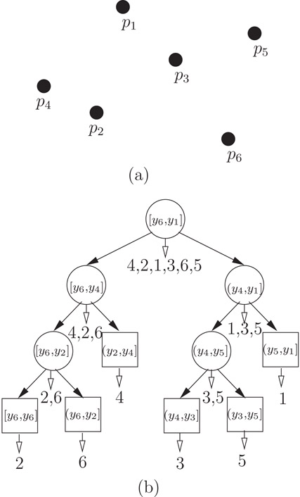
Figure 19.32D-range tree of S = {p1, p2, …, p6}, where p_i = (x_i, y_i).

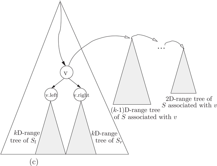
Figure 19.4A schematic representation of a (layered) kD-range tree, where S is the set associated with node v.

As this is a recursive algorithm with two parameters, k and |S|, that determine the recursion depth, it is not immediately obvious how much time and how much space are needed to construct a kD-range tree for a set of n points in k-dimensional space.

Let T(n, k) denote the time taken and S(n, k) denote the space required to build a kD-range tree of a set of n points in ℜk. The following are recurrence relations for T(n, k) and S(n, k), respectively.

T (n, k) = ⎧ ⎩ ⎨ ⎪ ⎪ O (1) O (n log n) 2 T (n / 2, k) + T (n, k - 1) + O (n) if n = 1 if k = 1 otherwise .

$T (n, k) = {\begin{cases} O (1) & if n = 1 \\ O (n \log n) & if k = 1 \\ 2 T (n / 2, k) + T (n, k - 1) + O (n) & otherwise . \end{cases}$

S (n, k) = ⎧ ⎩ ⎨ ⎪ ⎪ O (1) O (n) 2 S (n / 2, k) + S (n, k - 1) + O (1) if n = 1 if k = 1 otherwise .

$S (n, k) = {\begin{cases} O (1) & if n = 1 \\ O (n) & if k = 1 \\ 2 S (n / 2, k) + S (n, k - 1) + O (1) & otherwise . \end{cases}$

Note that in one dimension, we need to have the points sorted and stored in a sorted array, and thus T(n, 1) = O(n log n) and S(n, 1) = O(n). The solutions of T(n, k) and S(n, k) to the above recurrence relations are T(n, k) = O(n log^k−1n + n log n) for k ≥ 1 and S(n, k) = O(n log^k−1n) for k ≥ 1. For a general multidimensional divide-and-conquer scheme, and solutions to the recurrence relation, please refer to Bentley [19] and Monier [20], respectively.

We conclude that

Theorem 19.5

The kD-range tree for a set of n points in k-dimensional space can be constructed in O(n log^k−1n + n log n) time and O(n log^k−1n) space for k ≥ 1.

19.4.2Examples and Its Applications

Figure 19.3b illustrates an example of a range tree for a set of points in two dimensions, shown in Figure 19.3a. This list of integers under each node represents the indexes of points in ascending x-coordinates. Figure 19.4 illustrates a general schematic representation of a kD-range tree, which is a layered structure [3,4].

We now discuss how we make use of a range tree to solve the range search problem. We shall use 2D-range tree as an example for illustration purposes. It is rather obvious to generalize it to higher dimensions. Recall we have a set S of n points in the plane ℜ2 and 2D range query Q = [x_ℓ, x_r] × [y_ℓ, y_r]. Let us assume that a 2D-range tree rooted at 2D_Range_Tree_root(S) is available. Besides, for each node v in the range tree, it is associated with a standard range for the set S_v of points represented in the subtree rooted at node v, in this case [v.B, v.E] where v.B=min{pi.y} $v . B = min {p_{i} . y}$ and v.E=max{pi.y} $v . E = max {p_{i} . y}$ for all p_i ∈ S_v. v.key will split the standard range into two standard subranges [v.B, v.key] and [v.key, v.E], each associated with the root nodes v.left and v.right of the left and right subtrees of v, respectively.

The following pseudo code reports in F the set of points in S that lie in the range Q = [x_ℓ, x_r] × [y_ℓ, y_r]. It is invoked by 2D_Range_Search(v, x_ℓ, x_r, y_ℓ, y_r, F), where v is the root, 2D_Range_Tree_root(S), and F, initially empty, will return all the points in S that lie in the range Q = [x_ℓ, x_r] × [y_ℓ, y_r].

procedure 2D_Range_Search(v, x_ℓ, x_r, y_ℓ, y_r, F)

/* It returns F containing all the points in the range tree rooted at node v that lie in [x_ℓ, x_r] × [y_ℓ, y_r]. */

Input: A set S of n points in ℜ2, S = {p_i|i = 1, 2, …, n} and each point p_i = (p_i.x, p_i.y), where p_i.x and p_i.y are the x- and y-coordinates of p_i, p_i.x, p_i.y ∈ ℜ, i = 1, 2, …, n.

Output: A set F of points in S that lie in [x_ℓ, x_r] × [y_ℓ, y_r].

Method:

1.Start from the root node v to find the split node s, s = Find_split-node(v, y_ℓ, y_r) (see below), such that s.key lies in [y_ℓ, y_r].

2.if s is a leaf then 1D_Range_Search(s.aux, x_ℓ, x_r, F) that checks in the sorted array pointed to by s.aux, which contains just a point p, to see if its x-coordinate p.x lies in the x-range [x_ℓ, x_r].

3.v = s.left.

4.while v is not a leaf do

       if (y_ℓ ≤ v.key) then
              1D_Range_Search(v.right.aux, x_ℓ, x_r, F)
              v = v.left
       else v = v.right

5.(/* v is a leaf, and check node v.aux directly */)

1D_Range_Search(v.aux, x_ℓ, x_r, F)

6.v = s.right

7.while v is not a leaf do

       if (y_r > v.key) then
              1D_Range_Search(v.left.aux, x_ℓ, x_r, F)
              v = v.right
       else v = v.left

8.(/* v is a leaf, and check node v.aux directly */)

1D_Range_Search(v.aux, x_ℓ, x_r, F).

function Find_split-node(v, b, e)

/* Given a kD-range tree T rooted at v and an interval I = [b, e] ⊆ [v.B, v.E], this procedure returns the split-node s such that either [s.B, s.E] = [b, e] or [s_ℓ.B, s_ℓ.E] ∩ [b, e] ≠ ∅ and [s_r.B, s_r.E] ∩ [b, e] ≠ ∅, where s_ℓ and s_r are the left child and right child of s, respectively. */

1.if [v.B, v.E] = [b, e] then return v

2.if (b < v.key) and (e > v.key) then return v

3.if (e ≤ v.key) then return Find_split-node(v.left, b, e)

4.if (b ≥ v.key) then return Find_split-node(v.right, b, e)

procedure 1D_Range_Search(v, x_ℓ, x_r, F) is very straightforward. v is a pointer to a sorted array SA. We first do a binary search in SA looking for the first element no less than x_ℓ and then start to report in F those elements no greater than x_r. It is obvious that procedure 2D_Range_Search finds all the points in Q in O( log2n) time. Note that there are O(log n) nodes for which we need to invoke 1D_Range_Search in their auxiliary sorted arrays. These nodes v are in the canonical covering* of the y-range [y_ℓ, y_r], since its associated standard range [v.B, v.E] is totally contained in [y_ℓ, y_r], and the 2D-range search problem is now reduced to the 1D-range search problem.

This is not difficult to see that the 2D-range search problem can be answered in time O( log2n) plus time for output, as there are O(log n) nodes in the canonical covering of a given y-range and for each node in the canonical covering we spend O(log n) time for dealing with the 1D-range search problem.

However, with a modification to the auxiliary data structure, one can achieve an optimal query time of O(log n), instead of O( log2n) [18,21,22]. This is based on the observation that in each of the 1D-range search subproblem associated with each node in the canonical covering, we perform the same query, reporting points whose x-coordinates lie in the x-range [x_ℓ, x_r]. More specifically, we are searching for the smallest element no less than x_ℓ.

The modification is performed on the sorted array associated with each of the node in the 2D_Range_Tree(S).

Consider the root node v. As it is associated with the entire set of points, v.aux points to the sorted array containing the x-coordinates of all the points in S. Let this sorted array be denoted SA(v) and the entries, SA(v)_i, i = 1, 2, …, |S|, are sorted in nondecreasing order of the x-coordinate values. In addition to the x-coordinate value, each entry also contains the index of the corresponding point. That is, SA(v)_i.key and SA(v)_i.index contain the x-coordinate and index of p_j, respectively, where SA(v)_i.index = j and SA(v)_i.key = p_j.x.

We shall augment each entry SA(v)_i with two pointers, SA(v)_i.left and SA(v)_i.right. They are defined as follows. Let v_ℓ and v_r denote the roots of the left and right subtrees of v, that is, v.left = v_ℓ and v.right = v_r. SA(v)_i.left points to the entry SA(v_ℓ)_j such that entry SA(v_ℓ)_j.key is the smallest among all key values SA(v_ℓ)_j.key ≥ SA(v)_i.key. Similarly, SA(v)_i.right points to the entry SA(v_r)_k such that entry SA(v_r)_k.key is the smallest among all key values SA(v_r)_k.key ≥ SA(v)_i.key.

These two augmented pointers, SA(v)_i.left and SA(v)_i.right, possess the following property: if SA(v)_i.key is the smallest key such that SA(v)_i.key ≥ x_ℓ, then SA(v_ℓ)_j.key is also the smallest key such that SA(v_ℓ)_j.key ≥ x_ℓ. Similarly SA(v_r)_k.key is the smallest key such that SA(v_r)_k.key ≥ x_ℓ.

Thus if we have performed a binary search in the auxiliary sorted array SA(v) associated with node v locating the entry SA(v)_i whose key SA(v)_i.key is the smallest key such that SA(v)_i.key ≥ x_ℓ, then following the left (respectively right) pointer SA(v)_i.left (respectively SA(v)_i.right) to SA(v_ℓ)_j (respectively SA(v_r)_k), the entry SA(v_ℓ)_j.key (respectively SA(v_r)_k.key) is also the smallest key such that SA(v_ℓ)_j.key ≥ x_ℓ (respectively SA(v_r)_k.key ≥ x_ℓ). Thus there is no need to perform an additional binary search in the auxiliary sorted array SA(v.left) (respectively SA(v.right)).

With this additional modification, we obtain an augmented 2D-range tree and the following theorem.

Theorem 19.6

The 2D-range search problem for a set of n points in the two-dimensional space can be solved in time O(log n) plus time for output, using an augmented 2D-range tree that requires O(n log n) space.

The following procedure is generalized from procedure 2D_Range_Search(v, x_ℓ, x_r, y_ℓ, y_r, F) discussed in Section 19.4.2 taken into account the augmented auxiliary data structure. It is invoked by kD_Range_Search(k, v, Q, F), where v is the root kD_Range_Tree_root(S) of the range tree, Q is the kD-range, [x1ℓ,x1r]×[x2ℓ,x2r]×⋯×[xkℓ,xkr] $[x_{ℓ}^{1}, x_{r}^{1}] \times [x_{ℓ}^{2}, x_{r}^{2}] \times \dots \times [x_{ℓ}^{k}, x_{r}^{k}]$ , represented by a two dimensional array, such that Qi.ℓ=xiℓ $Q_{i} . ℓ = x_{ℓ}^{i}$ and Qi.r=xir $Q_{i} . r = x_{r}^{i}$ , and F, initially empty, will contain all the points that lie in Q.

procedure kD_Range_Search(k, v, Q, F).

/* It returns F containing all the points in the range tree rooted at node v that lie in kD-range, [x1ℓ,x1r]×[x2ℓ,x2r]×⋯×[xkℓ,xkr] $[x_{ℓ}^{1}, x_{r}^{1}] \times [x_{ℓ}^{2}, x_{r}^{2}] \times \dots \times [x_{ℓ}^{k}, x_{r}^{k}]$ , where each range [xiℓ,xir],xiℓ=Qi.ℓ,xir=Qi.r∈R,xiℓ≤xir $[x_{ℓ}^{i}, x_{r}^{i}], x_{ℓ}^{i} = Q_{i} . ℓ, x_{r}^{i} = Q_{i} . r \in ℜ, x_{ℓ}^{i} \leq x_{r}^{i}$ for all i = 1, 2, …, k denotes an interval in ℜ. */

Input: A set S of n points in ℜk, S = {p_i|i = 1, 2, …, n} and each point p_i = (p_i.x1, p_i.x2, …, p_i.xk), where p_i.xj ∈ ℜ, are the jth coordinates of p_i, j = 1, 2, …, k.

Output: A set F of points in S that lie in [x1ℓ,x1r]×[x2ℓ,x2r]×⋯×[xkℓ,xkr] $[x_{ℓ}^{1}, x_{r}^{1}] \times [x_{ℓ}^{2}, x_{r}^{2}] \times \dots \times [x_{ℓ}^{k}, x_{r}^{k}]$ .

Method:

1.if (k > 2) then

•Start from the root node v to find the split node s, s = Find_split-node(v, Q_k.ℓ, Q_k.r), such that s.key lies in [Q_k.ℓ, Q_k.r].

•if the split node is not found then return

•if s is a leaf then check in the sorted array pointed to by s.aux, which contains just a point p. p ⇒ F if its coordinate values lie in Q. return

•v = s.left

•while v is not a leaf do

          if (Q_k.ℓ ≤ v.key)
          then kD_Range_Search(k − 1, v.right.aux, Q, F)
             v = v.left
          else v = v.right

•(/* v is a leaf, and check node v.aux directly */)

Check in the sorted array pointed to by v.aux, which contains just a point p. p ⇒ F if its coordinate values lie in Q.

•v = s.right

•while v is not a leaf do

          if (Q_k.r > v.key)
          then kD_Range_Search(k − 1, v.left.aux, Q, F)
             v = v.right
          else v = v.left

•(/* v is a leaf, and check node v.aux directly */)

Check in the sorted array pointed to by v.aux, which contains just a point p. p ⇒ F if its coordinate values lie in Q.

2.else /* k ≤ 2*/

3.if k = 2 then

•Do binary search in sorted array SA(v) associated with node v, using Q1.ℓ (x1ℓ $x_{ℓ}^{1}$ ) as key to find entry o_v such that SA(v)ov $S A (v)_{o_{v}}$ ’s key, SA(v)ov.key $S A (v)_{o_{v}} . k e y$ is the smallest such that SA(v)ov.key≥Q1.ℓ $S A (v)_{o_{v}} . k e y \geq Q_{1} . ℓ$ .

•Find the split node s, s = Find_split-node(v, Q2.ℓ, Q2.r), such that s.key lies in [Q2.ℓ, Q2.r]. Record the root-to-split-node path from v to s, following left or right tree pointers.

•if the split node is not found then return

•Starting from entry o_v (SA(v)_i) follow pointers SA(v)ov.left $S A (v)_{o_{v}} . left$ or SA(v)ov.right $S A (v)_{o_{v}} . right$ according to the v-to-s path to point to entry SA(s)os $S A (s)_{o_{s}}$ associated with SA(s).

•if s is a leaf then check in the sorted array pointed to by s.aux, which contains just a point p. p ⇒ F if its coordinate values lie in Q. return

•v = s.left, ov=SA(s)os.left $o_{v} = S A (s)_{o_{s}} . left$

•while v is not a leaf do

          if (Q2.ℓ ≤ v.key)
          then ℓ=SA(v)ov.right $ℓ = S A (v)_{o_{v}} . right$ 
            while (SA(v.right)_ℓ.key ≤ Q1.r) do
              point p_m ⇒ F, where m = SA(v.right)_ℓ.index
              ℓ++
            v = v.left, ov=SA(v)ov.left $o_{v} = S A (v)_{o_{v}} . left$ 
          else v = v.right, ov=SA(v)ov.right $o_{v} = S A (v)_{o_{v}} . right$

•(/* v is a leaf, and check node v.aux directly */)

Check in the sorted array pointed to by v.aux, which contains just a point p. p ⇒ F if its coordinate values lie in Q.

•v = s.right, ov=SA(s)os.right $o_{v} = S A (s)_{o_{s}} . right$

•while v is not a leaf do

          if (Q2.r > v.key)
          then ℓ=SA(v)ov.left $ℓ = S A (v)_{o_{v}} . left$ 
            while (SA(v.left)_ℓ.key ≤ Q1.r) do
             point p_m⇒F, where m = SA(v.left)_ℓ.index
             ℓ++
            v = v.right, ov=SA(v)ov.right $o_{v} = S A (v)_{o_{v}} . right$ 
          else v = v.left, ov=SA(v)ov.left $o_{v} = S A (v)_{o_{v}} . left$

•(/* v is a leaf, and check node v.aux directly */)

Check in the sorted array pointed to by v.aux, which contains just a point p. p ⇒ F if its coordinate values lie in Q.

The following recurrence relation for the query time Q(n, k) of the kD-range search problem can be easily obtained:

Q (n, k) = ⎧ ⎩ ⎨ ⎪ ⎪ O (1) O (log n) + F Σ v \in C C Q (n v, k - 1) + O (log n) if n = 1 if k = 2 otherwise

$Q (n, k) = {\begin{cases} O (1) & if n = 1 \\ O (\log n) + F & if k = 2 \\ Σ_{v \in C C} Q (n_{v}, k - 1) + O (\log n) & otherwise \end{cases}$

where F $F$ denotes the output size and n_v denotes the size of the subtree rooted at node v that belongs to the canonical covering CC of the query. The solution is Q(n,k)=O(logk−1n)+F $Q (n, k) = O (\log^{k - 1} n) + F$ [3,4].

We conclude with the following theorem.

Theorem 19.7

The kD-range search problem for a set of n points in the k-dimensional space can be solved in time O( log^k−1n) plus time for output, using an augmented kD-range tree that requires O(n log^k−1n) space for k ≥ 1.

19.5Priority Search Trees

The priority search tree was originally introduced by McCreight [23]. It is a hybrid of two data structures, binary search tree and a priority queue [24]. A priority queue is a queue and supports the following operations: insertion of an item and deletion of the minimum (highest priority) item, so called delete_min operation. Normally the delete_min operation takes constant time, while updating the queue so that the minimum element is readily accessible takes logarithmic time. However, searching for an element in a priority queue will normally take linear time. To support efficient searching, the priority queue is modified to be a priority search tree. We will give a formal definition and its construction later. As the priority search tree represents a set S of elements, each of which has two pieces of information, one being a key from a totally ordered set, say the set ℜ of real numbers, and the other being a notion of priority, also from a totally ordered set, for each element, we can model this set S as a set of points in two-dimensional space. The x- and y-coordinates of a point p represent the key and the priority, respectively. For instance, consider a set of jobs S = {J1, J2, …, J_n}, each of which has a release time r_i ∈ ℜ and a priority p_i ∈ ℜ, i = 1, 2, …, n. Then each job J_i can be represented as a point q such that q.x = r_i, q.y = p_i.

The priority search tree can be used to support queries of the form, find, among a set S of n points, the point p with minimum p.y such that its x-coordinate lies in a given range [ℓ, r], that is, ℓ ≤ p.x ≤ r. As can be shown later, this query can be answered in O(log n) time.

19.5.1Construction of Priority Search Trees

As before, the root node, Priority_Search_Tree_root(S), represents the entire set S of points. Each node v in the tree will have a key v.key, an auxiliary data v.aux containing the index of the point, and two pointers v.left and v.right to its left and right subtrees, respectively, such that all the key values stored in the left subtree are less than v.key and all the key values stored in the right subtree are greater than v.key. The following is a pseudo code for the recursive construction of the priority search tree of a set S of n points in ℜ2. See Figure 19.5a for an illustration.

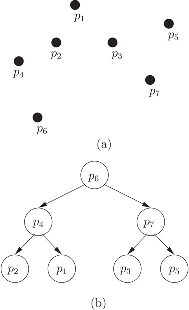
Figure 19.5Priority search tree of S = {p1, p2, …, p7}.

function Priority_Search_Tree(S)

/* It returns a pointer v to the root, Priority_Search_Tree_root(S), of the priority search tree for a set S of points. */

Input: A set S of n points in ℜ2, S = {p_i|i = 1, 2, …, n} and each point p_i = (p_i.x, p_i.y), where p_i.x and p_i.y are the x- and y-coordinates of p_i, p_i.x, p_i.y ∈ ℜ, i = 1, 2, …, n.

Output: A priority search tree, rooted at Priority_Search_Tree_root(S).

Method:

1.if S = ∅, return nil.

2.Create a node v such that v.key equals the median of the set {p.x|p ∈ S}, and v.aux contains the index i of the point p_i whose y-coordinate is the minimum among all the y-coordinates of the set S of points, that is, pi.y=min{p.y|p∈S} $p_{i} . y = min {p . y | p \in S}$ .

3.Let Sℓ={p∈S{pv.aux}|p.x≤v.key} $S_{ℓ} = {p \in S {p_{v . a u x}} | p . x \leq v . k e y}$ and Sr={p∈S{pv.aux}|p.x>v.key} $S_{r} = {p \in S {p_{v . a u x}} | p . x > v . k e y}$ denote the set of points whose x-coordinates are less than or equal to v.key and greater than v.key, respectively.

4.v.left= Priority_Search_Tree(S_ℓ).

5.v.right= Priority_Search_Tree(S_r).

6.return v.

Thus, Priority_Search_Tree_root(S) is a minimum heap data structure with respect to the y-coordinates, that is, the point with minimum y-coordinate can be accessed in constant time, and is a balanced binary search tree for the x-coordinates. Implicitly the root node v is associated with an x-range [x_ℓ, x_r] representing the span of the x-coordinate values of all the points in the whole set S. The root of the left subtree pointed to by v.left is associated with the x-range [x_ℓ, v.key] representing the span of the x-coordinate values of all the points in the set S_ℓ and the root of the right subtree pointed to by v.right is associated with the x-range (v.key, x_r] representing the span of the x-coordinate values of all the points in the set S_r. It is obvious that this algorithm takes O(n log n) time and linear space. We summarize this in the following.

Theorem 19.8

The priority search tree for a set S of n points in ℜ2 can be constructed in O(n log n) time and linear space.

19.5.2Examples and Its Applications

Figure 19.5 illustrates an example of a priority search tree of the set of points. Note that the root node contains p6 since its y-coordinate value is the minimum.

We now illustrate a usage of the priority search tree by an example. Consider a so-called grounded 2D-range search problem for a set of n points in the plane. As defined in Section 19.4.2, a 2D-range search problem is to find all the points p ∈ S such that p.x lies in an x-range [x_ℓ, x_r], x_ℓ ≤ x_r and p.y lies in a y-range [y_ℓ, y_r]. When the y-range is of the form [ − ∞, y_r] then the 2D-range is referred to as grounded 2D-range or sometimes as 1.5D-range, and the 2D-range search problem as grounded 2D-range search or 1.5D-range search problem.

Grounded 2D-Range Search Problem: Given a set S of n points in the plane ℜ2, with preprocessing allowed, find the subset F of points whose x- and y-coordinates satisfy a grounded 2D-range query of the form [x_ℓ, x_r] × [−∞, y_r], x_ℓ, x_r, y_r ∈ ℜ, x_ℓ ≤ x_r.

The following pseudo code solves this problem optimally. We assume that a priority search tree for S has been constructed via procedure Priority_Search_Tree(S). The answer will be obtained in F via an invocation to Priority_Search_Tree_Range_Search(v, x_ℓ, x_r, y_r, F), where v is Priority_Search_Tree_root(S).

procedure Priority_Search_Tree_Range_Search(v, x_ℓ, x_r, y_r, F)

/* v points to the root of the tree, F is a queue and set to nil initially. */

Input: A set S of n points, {p1, p2, …, p_n}, in ℜ2, stored in a priority search tree, Priority_Search_Tree(S) pointed to by Priority_Search_Tree_root(S), and a grounded 2D-range [x_ℓ, x_r] × [−∞, y_r], x_ℓ, x_r, y_r ∈ ℜ, x_ℓ ≤ x_r.

Output: A subset F ⊆ S of points that lie in the grounded 2D-range, that is, F = {p ∈ S|x_ℓ ≤ p.x ≤ x_r and p.y ≤ y_r}.

Method:

1.Start from the root v finding the first split node v_split such that v_split.key lies in the x-range [x_ℓ, x_r].

2.For each node u on the path from node v to node v_split, if the point p_u.aux lies in range [x_ℓ, x_r] × [−∞, y_r] then report it by (p_u.aux⇒F).

3.For each node u on the path from v_split.left to x_ℓ in the left subtree of v_split, do

if the path goes left at u then Priority_Search_Tree_1dRange_Search(u.right, y_r, F)

4.For each node u on the path from v_split.right to x_r in the right subtree of v_split, do

if the path goes right at u then Priority_Search_Tree_1dRange_Search(u.left, y_r, F)

procedure Priority_Search_Tree_1dRange_Search(v, y_r, F)

/* Report in F all the points p_i, whose y-coordinate values are no greater than y_r, where i = v.aux. */

1.if v is nil, return.

2.if pv.aux.y≤yr $p_{v . a u x} . y \leq y_{r}$ then report it by (p_v.aux ⇒ F).

3.Priority_Search_Tree_1dRange_Search(v.left, y_r, F)

4.Priority_Search_Tree_1dRange_Search(v.right, y_r, F)

procedure Priority_Search_Tree_1dRange_Search(v, y_r, F) basically retrieves all the points stored in the priority search tree rooted at v such that their y-coordinates are all less than or equal to y_r. The search terminates at the node u whose associated point has a y-coordinate greater than y_r, implying all the nodes in the subtree rooted at u satisfy this property. The amount of time required is proportional to the output size. Thus we conclude that

Theorem 19.9

The Grounded 2D-Range Search Problem for a set S of n points in the plane ℜ2 can be solved in time O( log n) plus time for output, with a priority search tree structure for S that requires O(n log n) time and O(n) space.

Note that the space requirement for the priority search tree is linear, compared to that of a 2D-range tree, which requires O(n log n) space. That is, the Grounded 2D-Range Search Problem for a set S of n points can be solved optimally using priority search tree structure.

Acknowledgments

This work was supported in part by the National Science Council under the grants NSC-91-2219-E-001-001, NSC91-2219-E-001-002, and by the Ministry of Science and Technology under the grants MOST 104–2221-E-001-031 and MOST 104–2221-E-001-032.

References

1.H. Imai and Ta. Asano, Finding the connected components and a maximum clique of an intersection graph of rectangles in the plane, J. Algorithms, vol. 4, 1983, pp. 310–323.

2.D. T. Lee, Maximum clique problem of rectangle graphs, in Advances in Computing Research, Vol. 1, ed. F.P. Preparata, JAI Press Inc., Greenwich, CT, 1983, 91–107.

3.M. de Berg, M. van Kreveld, M. Overmars and O. Schwarzkopf, Computational Geometry: Algorithms and Applications, Springer-Verlag, Berlin, 1997.

4.F. P. Preparata and M. I. Shamos, Computational Geometry: An Introduction, 3rd edition, Springer-Verlag, 1990.

5.J. L. Bentley, Decomposable searching problems, Inform. Process Lett., vol. 8, 1979, pp. 244–251.

6.J. L. Bentley and J. B. Saxe, Decomposable searching problems. I: Static-to-dynamic transformation, J. Algorithms, vol. 1, 1980, pp. 301–358.

7.M. H. Overmars and J. van Leeuwen, Two general methods for dynamizing decomposable searching problems, Computing, vol. 26, 1981, pp. 155–166.

8.H. Edelsbrunner, A new approach to rectangle intersections. Part I, Intl. J. Comput. Math., vol. 13, 1983, pp. 209–219.

9.H. Edelsbrunner, A new approach to rectangle intersections. Part II, Intl. J. Comput. Math., vol. 13, 1983, pp. 221–229.

10.P. Gupta, R. Janardan, M. Smid and B. Dasgupta, The rectangle enclosure and point-dominance problems revisited, Intl. J. Comput. Geom. Appl., vol. 7, 1997, pp. 437–455.

11.D. T. Lee and F. P. Preparata, An improved algorithm for the rectangle enclosure problem, J. Algorithms, vol. 3, 1982, pp. 218–224.

12.J.-D. Boissonnat and F. P. Preparata, Robust plane sweep for intersecting segments, SIAM J. Comput., vol. 295, 2000, pp. 1401–1421.

13.M. L. Fredman and B. Weide, On the complexity of computing the measure of ∪[a_i, b_i], Commun. ACM, vol. 21, 1978, pp. 540–544.

14.J. van Leeuwen and D. Wood, The measure problem for rectangular ranges in d-space, J. Algorithms, vol. 2, 1981, pp. 282–300.

15.U. Gupta, D. T. Lee and J. Y-T. Leung, An optimal solution for the channel-assignment problem, IEEE Trans. Comput., vol. 28(11), 1979, pp. 807–810.

16.M. Sarrafzadeh and D. T. Lee, Restricted track assignment with applications, Intl. J. Comput. Geom. Appl., vol. 4, 1994, pp. 53–68.

17.G. S. Lueker and D. E. Willard, A data structure for dynamic range queries, Inform. Process. Lett., vol. 15, 1982, pp. 209–213.

18.D. E. Willard, New data structures for orthogonal range queries, SIAM J. Comput., vol. 14, 1985, pp. 232–253.

19.J. L. Bentley, Multidimensional divide-and-conquer, Commun. ACM, vol. 23,4, 1980, pp. 214–229.

20.L. Monier, Combinatorial solutions of multidimensional divide-and-conquer recurrences, J. Algorithms, vol. 1, 1980, pp. 60–74.

21.B. Chazelle and L. J. Guibas, Fractional cascading. I: A data structuring technique, Algorithmica, vol. 13, 1986, pp. 133–162.

22.B. Chazelle and L. J. Guibas, Fractional cascading. II: Applications, Algorithmica, vol. 1, 1986, pp. 163–191.

23.E. M. McCreight, Priority search trees, SIAM J. Comput., vol. 14, 1985, pp. 257–276.

24.E. Horowitz, S. Sahni and S. Anderson-Freed, Fundamentals of Data Structures in C, Computer Science Press, 1993.

*A rectangle intersection graph is a graph G = (V, E), in which each vertex in V corresponds to a rectangle, and two vertices are connected by an edge in E, if the corresponding rectangles intersect.

†A searching problem is said to be decomposable if and only if ∀x∈T1,A,B∈2T2,Q(x,A∪B)=◯(Q(x,A),Q(x,B)) $\forall x \in T_{1}, A, B \in 2^{T_{2}}, Q (x, A \cup B) = ◯ (Q (x, A), Q (x, B))$ for some efficiently computable associative operator ◯ $◯$ on the elements of T3, where Q is a mapping from T1 × 2^T2 to T3 [5,6].

*See the definition of the canonical covering defined in Section 19.3.1.

..................Content has been hidden....................

You can't read the all page of ebook, please click here login for view all page.

Table of Contents for 19. Interval, Segment, Range, Priority Search Trees

Create new playlist

Sign In

Sign Up

Table of Contents for
19. Interval, Segment, Range, Priority Search Trees