
Multidimensional Spatial Data Structures
Hanan Samet*
University of Maryland at College Park
17.6Line Data and Boundaries of Regions
17.7Research Issues and Summary
The representation of multidimensional data is an important issue in applications in diverse fields that include database management systems (see Chapter 62), computer graphics (see Chapter 55), computer vision, computational geometry (see Chapters 65, 66 and 67), image processing (see Chapter 58), geographic information systems (GIS) (see Chapter 56), pattern recognition, VLSI design (Chapter 53), and others. The most common definition of multidimensional data is a collection of points in a higher dimensional space. These points can represent locations and objects in space as well as more general records where only some, or even none, of the attributes are locational. As an example of nonlocational point data, consider an employee record which has attributes corresponding to the employee’s name, address, sex, age, height, weight, and social security number. Such records arise in database management systems and can be treated as points in, for this example, a seven-dimensional space (i.e., there is one dimension for each attribute) albeit the different dimensions have different type units (i.e., name and address are strings of characters, sex is binary; while age, height, weight, and social security number are numbers).
When multidimensional data corresponds to locational data, we have the additional property that all of the attributes have the same unit which is distance in space. In this case, we can combine the distance-denominated attributes and pose queries that involve proximity. For example, we may wish to find the closest city to Chicago within the two-dimensional space from which the locations of the cities are drawn. Another query seeks to find all cities within 50 miles of Chicago. In contrast, such queries are not very meaningful when the attributes do not have the same type.
When multidimensional data spans a continuous physical space (i.e., an infinite collection of locations), the issues become more interesting. In particular, we are no longer just interested in the locations of objects, but, in addition, we are also interested in the space that they occupy (i.e., their extent). Some example objects include lines (e.g., roads, rivers), regions (e.g., lakes, counties, buildings, crop maps, polygons, polyhedra), rectangles, and surfaces. The objects may be disjoint or could even overlap. One way to deal with such data is to store it explicitly by parameterizing it and thereby reduce it to a point in a higher dimensional space. For example, a line in two-dimensional space can be represented by the coordinate values of its endpoints (i.e., a pair of x and a pair of y coordinate values) and then stored as a point in a four-dimensional space [1]. Thus, in effect, we have constructed a transformation (i.e., mapping) from a two-dimensional space (i.e., the space from which the lines are drawn) to a four-dimensional space (i.e., the space containing the representative point corresponding to the line).
The transformation (also known as parameterization) approach is fine if we are just interested in retrieving the data. It is appropriate for queries about the objects (e.g., determining all lines that pass through a given point or that share an endpoint, etc.) and the immediate space that they occupy. However, the drawback of the transformation approach is that it ignores the geometry inherent in the data (e.g., the fact that a line passes through a particular region) and its relationship to the space in which it is embedded.
For example, suppose that we want to detect if two lines are near each other, or, alternatively, to find the nearest line to a given line. This is difficult to do in the four-dimensional space, regardless of how the data in it is organized, since proximity in the two-dimensional space from which the lines are drawn is not necessarily preserved in the four-dimensional space into which the lines have been transformed. In other words, although the two lines may be very close to each other, the Euclidean distance between their representative points may be quite large, unless the lines are approximately the same size, in which case proximity is preserved [2].
Of course, we could overcome these problems by projecting the lines back to the original space from which they were drawn, but in such a case, we may ask what was the point of using the transformation in the first place? In other words, at the least, the representation that we choose for the data should facilitate the performance of operations on the data. Thus when the multidimensional spatial data is nondiscrete, we need representations besides those that are designed for point data. The most common solution, and the one that we focus on in the rest of this chapter, is to use data structures that are based on spatial occupancy. Such methods decompose the space from which the spatial data is drawn (e.g., the two-dimensional space containing the lines) into regions that are usually called buckets because they often contain more than just one element. They are also commonly known as bucketing methods.
In this chapter, we explore a number of different representations of multidimensional data bearing the above issues in mind. While we cannot give exhaustive details of all of the data structures, we try to explain the intuition behind their development as well as to give literature pointers to where more information can be found. Many of these representations are described in greater detail in References 3–5 including an extensive bibliography. Our approach is primarily a descriptive one. Most of our examples are of two-dimensional spatial data although the representations are applicable to higher dimensional spaces as well.
At times, we discuss bounds on execution time and space requirements. Nevertheless, this information is presented in an inconsistent manner. The problem is that such analyses are very difficult to perform for many of the data structures that we present. This is especially true for the data structures that are based on spatial occupancy (e.g., quadtree [see Chapter 20 for more details] and R-tree [see Chapter 22 for more details) variants). In particular, such methods have good observable average-case behavior but may have very bad worst cases which may only arise rarely in practice. Their analysis is beyond the scope of this chapter and usually we do not say anything about it. Nevertheless, these representations find frequent use in applications where their behavior is deemed acceptable, and is often found to be better than that of solutions whose theoretical behavior would appear to be superior. The problem is primarily attributed to the presence of large constant factors which are usually ignored in the big O and Ω analyses [6].
The rest of this chapter is organized as follows. Section 17.2 reviews a number of representations of point data of arbitrary dimensionality. Section 17.3 describes bucketing methods that organize collections of spatial objects (as well as multidimensional point data) by aggregating the space that they occupy. The remaining sections focus on representations of nonpoint objects of different types. Section 17.4 covers representations of region data, while Section 17.5 discusses a subcase of region data which consists of collections of rectangles. Section 17.6 deals with curvilinear data which also includes polygonal subdivisions and collections of line segments. Section 17.7 contains a summary and a brief indication of some research issues and directions for future work.
The simplest way to store point data of arbitrary dimension is in a sequential list. Accesses to the list can be sped up by forming sorted lists for the various attributes which are known as inverted lists [7]. There is one list for each attribute. This enables pruning the search with respect to the value of one of the attributes. It should be clear that the inverted list is not particularly useful for multidimensional range searches. The problem is that it can only speed up the search for one of the attributes (termed the primary attribute). A widely used solution is exemplified by the fixed-grid method [7,8]. It partitions the space from which the data is drawn into rectangular cells by overlaying it with a grid. Each grid cell c contains a pointer to another structure (e.g., a list) which contains the set of points that lie in c. Associated with the grid is an access structure to enable the determination of the grid cell associated with a particular point p. This access structure acts like a directory and is usually in the form of a d-dimensional array with one entry per grid cell or a tree with one leaf node per grid cell.
There are two ways to build a fixed grid. We can either subdivide the space into equal-sized intervals along each of the attributes (resulting in congruent grid cells) or place the subdivision lines at arbitrary positions that are dependent on the underlying data. In essence, the distinction is between organizing the data to be stored and organizing the embedding space from which the data is drawn [9]. In particular, when the grid cells are congruent (i.e., equal-sized when all of the attributes are locational with the same range and termed a uniform grid), use of an array access structure is quite simple and has the desirable property that the grid cell associated with point p can be determined in constant time. Moreover, in this case, if the width of each grid cell is twice the search radius for a rectangular range query, then the average search time is O(F · 2d) where F is the number of points that have been found [10]. Figure 17.1 is an example of a uniform-grid representation for a search radius equal to 10 (i.e., a square of size 20 × 20).
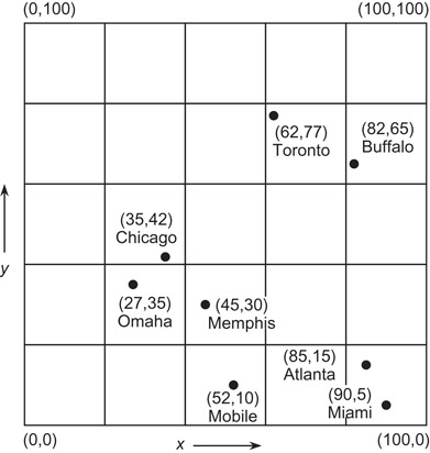
Figure 17.1Uniform-grid representation corresponding to a set of points with a search radius of 20.
The use of an array access structure when the grid cells are not congruent requires us to have a way of keeping track of their size so that we can determine the entry of the array access structure corresponding to the grid cell associated with point p. One way to do this is to make use of what are termed linear scales which indicate the positions of the grid lines (or partitioning hyperplanes in d > 2 dimensions). Given a point p, we determine the grid cell in which p lies by finding the “coordinate values” of the appropriate grid cell. The linear scales are usually implemented as one-dimensional trees containing ranges of values.
The array access structure is fine as long as the data is static. When the data is dynamic, it is likely that some of the grid cells become too full while other grid cells are empty. This means that we need to rebuild the grid (i.e., further partition the grid or reposition the grid partition lines or hyperplanes) so that the various grid cells are not too full. However, this creates many more empty grid cells as a result of repartitioning the grid (i.e., empty grid cells are split into more empty grid cells). The number of empty grid cells can be reduced by merging spatially adjacent empty grid cells into larger empty grid cells, while splitting grid cells that are too full, thereby making the grid adaptive. The result is that we can no longer make use of an array access structure to retrieve the grid cell that contains query point p. Instead, we make use of a tree access structure in the form of a k-ary tree where k is usually 2d. Thus what we have done is marry a k-ary tree with the fixed-grid method. This is the basis of the point quadtree [11] and the PR quadtree [4,12] which are multidimensional generalizations of binary trees.
The difference between the point quadtree and the PR quadtree is the same as the difference between trees and tries [13], respectively. The binary search tree [7] is an example of the former since the boundaries of different regions in the search space are determined by the data being stored. Address computation methods such as radix searching [7] (also known as digital searching) are examples of the latter, since region boundaries are chosen from among locations that are fixed regardless of the content of the data set. The process is usually a recursive halving process in one dimension, recursive quartering in two dimensions, and so on, and is known as regular decomposition.
In two dimensions, a point quadtree is just a two-dimensional binary search tree. The first point that is inserted serves as the root, while the second point is inserted into the relevant quadrant of the tree rooted at the first point. Clearly, the shape of the tree depends on the order in which the points were inserted. For example, Figure 17.2 is the point quadtree corresponding to the data of Figure 17.1 inserted in the order Chicago, Mobile, Toronto, Buffalo, Memphis, Omaha, Atlanta, and Miami.

Figure 17.2A point quadtree and the records it represents corresponding to Figure 17.1: (a) the resulting partition of space and (b) the tree representation.
In two dimensions, the PR quadtree is based on a recursive decomposition of the underlying space into four congruent (usually square in the case of locational attributes) cells until each cell contains no more than one point. For example, Figure 17.3a is the partition of the underlying space induced by the PR quadtree corresponding to the data of Figure 17.1, while Figure 17.3b is its tree representation. The shape of the PR quadtree is independent of the order in which data points are inserted into it. The disadvantage of the PR quadtree is that the maximum level of decomposition depends on the minimum separation between two points. In particular, if two points are very close, then the decomposition can be very deep. This can be overcome by viewing the cells or nodes as buckets with capacity c and only decomposing a cell when it contains more than c points.

Figure 17.3A PR quadtree and the points it represents corresponding to Figure 17.1: (a) the resulting partition of space, (b) the tree representation, and (c) one possible B+-tree for the nonempty grid cells where each node has a minimum of 2 and a maximum of 3 entries. The nonempty grid cells in (a) have been labeled with the name of the B+-tree leaf node in which they are a member.
As the dimensionality of the space increases, each level of decomposition of the quadtree results in many new cells as the fanout value of the tree is high (i.e., 2d). This is alleviated by making use of a k-d tree [14]. The k-d tree is a binary tree where at each level of the tree, we subdivide along a different attribute so that, assuming d locational attributes, if the first split is along the x-axis, then after d levels, we cycle back and again split along the x-axis. It is applicable to both the point quadtree and the PR quadtree (in which case we have a PR k-d tree, or a bintree in the case of region data).
At times, in the dynamic situation, the data volume becomes so large that a tree access structure such as the one used in the point and PR quadtrees is inefficient. In particular, the grid cells can become so numerous that they cannot all fit into memory thereby causing them to be grouped into sets (termed buckets) corresponding to physical storage units (i.e., pages) in secondary storage. The problem is that, depending on the implementation of the tree access structure, each time we must follow a pointer, we may need to make a disk access. Below, we discuss two possible solutions: one making use of an array access structure and one making use of an alternative tree access structure with a much larger fanout. We assume that the original decomposition process is such that the data is only associated with the leaf nodes of the original tree structure.
The difference from the array access structure used with the static fixed-grid method described earlier is that the array access structure (termed grid directory) may be so large (e.g., when d gets large) that it resides on disk as well, and the fact that the structure of the grid directory can change as the data volume grows or contracts. Each grid cell (i.e., an element of the grid directory) stores the address of a bucket (i.e., page) that contains the points associated with the grid cell. Notice that a bucket can correspond to more than one grid cell. Thus any page can be accessed by two disk operations: one to access the grid cell and one more to access the actual bucket.
This results in EXCELL [15] when the grid cells are congruent (i.e., equal-sized for locational data), and grid file [9] when the grid cells need not be congruent. The difference between these methods is most evident when a grid partition is necessary (i.e., when a bucket becomes too full and the bucket is not shared among several grid cells). In particular, a grid partition in the grid file only splits one interval in two thereby resulting in the insertion of a (d − 1)-dimensional cross-section. On the other hand, a grid partition in EXCELL means that all intervals must be split in two thereby doubling the size of the grid directory.
An alternative to the array access structure is to assign an ordering to the grid cells resulting from the adaptive grid, and then to impose a tree access structure on the elements of the ordering that correspond to the nonempty grid cells. The ordering is analogous to using a mapping from d dimensions to one dimension. There are many possible orderings (e.g., see chapter 2 in Reference 5) with the most popular shown in Figure 17.4.

Figure 17.4The result of applying four common different space-ordering methods to an 8 × 8 collection of pixels whose first element is in the upper left corner: (a) row order, (b) row-prime order, (c) Morton order, and (d) Peano–Hilbert order.
The domain of these mappings is the set of locations of the smallest possible grid cells (termed pixels) in the underlying space and thus we need to use some easily identifiable pixel in each grid cell such as the one in the grid cell’s lower left corner. Of course, we also need to know the size of each grid cell. One mapping simply concatenates the result of interleaving the binary representations of the coordinate values of the lower left corner (e.g., (a, b) in two dimensions) and i of each grid cell of size 2i so that i is at the right. The resulting number is termed a locational code and is a variant of the Morton order (Figure 17.4c). Assuming such a mapping and sorting the locational codes in increasing order yields an ordering equivalent to that which would be obtained by traversing the leaf nodes (i.e., grid cells) of the tree representation (e.g., Figure 17.8b) in the order SW, SE, NW, NE. It is also known as the Z-order on account of the Z-like pattern formed by the ordering. The Morton order (as well as the Peano–Hilbert order shown in Figure 17.4d) is particularly attractive for quadtree-like decompositions because all pixels within a grid cell appear in consecutive positions in the order. Alternatively, these two orders exhaust a grid cell before exiting it.
For example, Figure 17.3c shows the result of imposing a B+-tree [16] access structure on the nonempty grid cells of the PR quadtree given in Figure 17.3b. Each node of the B+-tree in our example has a minimum of 2 and a maximum of 3 entries. Figure 17.3c does not contain the values resulting from applying the mapping to the individual grid cells nor does it show the discriminator values that are stored in the nonleaf nodes of the B+-tree. The nonempty grid cells of the PR quadtree in Figure 17.3a are marked with the label of the leaf node of the B+-tree of which they are a member (e.g., the grid cell containing Chicago is in leaf node Q of the B+-tree).
It is important to observe that the above combination of the PR quadtree and the B+-tree has the property that the tree structure of the partition process of the underlying space has been decoupled [17] from that of the node hierarchy (i.e., the grouping process of the nodes resulting from the partition process) that makes up the original tree directory. More precisely, the grouping process is based on proximity in the ordering of the locational codes and on the minimum and maximum capacity of the nodes of the B+-tree. Unfortunately, the resulting structure has the property that the space that is spanned by a leaf node of the B+-tree (i.e., the grid cells spanned by it) has an arbitrary shape and, in fact, does not usually correspond to a k-dimensional hyperrectangle. In particular, the space spanned by the nonempty leaf node may have the shape of a staircase (e.g., the nonempty grid cells in Figure 17.3a that comprise leaf nodes S and T of the B+-tree in Figure 17.3c) or may not even be connected in the sense that it corresponds to regions that are not contiguous (e.g., the nonempty grid cells in Figure 17.3a that comprise the leaf node R of the B+-tree in Figure 17.3c). The PK-tree [18] is an alternative decoupling method which overcomes these drawbacks by basing the grouping process on k-instantiation which stipulates that each node of the grouping process contains a minimum of k objects or nonempty grid cells. The result is that all of the nonempty grid cells of the grouping process are congruent at the cost that the result is not balanced although use of relatively large values of k ensures that the resulting trees are relatively shallow or of a limited number of shapes. It can be shown that when the partition process has a fanout of f, then k-instantiation means that the number of objects in each node of the grouping process is bounded by f · (k − 1). Note that k-instantiation is different from bucketing where we only have an upper bound on the number of objects in the node.
Fixed-grids, quadtrees, k-d trees, grid file, EXCELL, as well as other hierarchical representations are good for range searching queries such as finding all cities within 80 miles of St. Louis. In particular, they act as pruning devices on the amount of search that will be performed as many points will not be examined since their containing cells lie outside the query range. These representations are generally very easy to implement and have good expected execution times, although they are quite difficult to analyze from a mathematical standpoint. However, their worst cases, despite being rare, can be quite bad. These worst cases can be avoided by making use of variants of range trees [19] and priority search trees [20]. For more details about these data structures, see Chapter 19.
There are four principal approaches to decomposing the space from which the objects are drawn. The first approach makes use of an object hierarchy and the space decomposition is obtained in an indirect manner as the method propagates the space occupied by the objects up the hierarchy with the identity of the propagated objects being implicit to the hierarchy. In particular, associated with each object is an object description (e.g., for region data, it is the set of locations in space corresponding to the cells that make up the object). Actually, since this information may be rather voluminous, it is often the case that an approximation of the space occupied by the object is propagated up the hierarchy rather than the collection of individual cells that are spanned by the object. For spatial data, the approximation is usually the minimum bounding rectangle formally known as the minimum axis-aligned bounding box (AABB) for the object, while for nonspatial data it is simply the hyperrectangle whose sides have lengths equal to the ranges of the values of the attributes. Therefore, associated with each element in the hierarchy is a bounding rectangle corresponding to the union of the bounding rectangles associated with the elements immediately below it.
The R-tree [21,22] (also sometimes referenced as an AABB tree) is an example of an object hierarchy which finds use especially in database applications. Note that other bounding objects can be used such as spheres (e.g., the SS-tree [23]), and the intersection of the minimum bounding sphere and the minimum bounding rectangle (e.g., the SR-tree [24]). Moreover, the minimum bounding rectangles need not be axis-aligned (e.g., the OBB-tree [25]). The number of objects or bounding rectangles that are aggregated in each node is permitted to range between a minimum of m where m ≤ ⌈M/2⌉ and a maximum of M. The root node in an R-tree has at least two entries unless it is a leaf node in which case it has just one entry corresponding to the bounding rectangle of an object. The R-tree is usually built dynamically as the objects are encountered rather than waiting until all objects have been input (dynamically). The hierarchy is implemented as a tree structure with grouping being based, in part, on proximity of the objects or bounding rectangles.
For example, consider the collection of line segment objects given in Figure 17.5 shown embedded in a 4 × 4 grid. Figure 17.6a is an example R-tree for this collection with m = 2 and M = 3. Figure 17.6b shows the spatial extent of the bounding rectangles of the nodes in Figure 17.6a, with heavy lines denoting the bounding rectangles corresponding to the leaf nodes, and broken lines denoting the bounding rectangles corresponding to the subtrees rooted at the nonleaf nodes. Note that the R-tree is not unique. Its structure depends heavily on the order in which the individual objects were inserted into (and possibly deleted from) the tree.

Figure 17.5Example collection of line segments embedded in a 4 × 4 grid.

Figure 17.6(a) R-tree for the collection of line segments with m = 2 and M = 3, in Figure 17.5, and (b) the spatial extents of the bounding rectangles. Notice that the leaf nodes in the index also store bounding rectangles although this is only shown for the nonleaf nodes.
Given that each R-tree node can contain a varying number of objects or bounding rectangles, it is not surprising that the R-tree was inspired by the B-tree [26]. Therefore, nodes are viewed as analogous to disk pages. Thus the parameters defining the tree (i.e., m and M) are chosen so that a small number of nodes is visited during a spatial query (i.e., point and range queries), which means that m and M are usually quite large. The actual implementation of the R-tree is really a B+-tree [16] as the objects are restricted to the leaf nodes.
The efficiency of the R-tree for search operations depends on its ability to distinguish between occupied space and unoccupied space (i.e., coverage), and to prevent a node from being examined needlessly due to a false overlap with other nodes. In other words, we want to minimize coverage and overlap. These goals guide the initial R-tree creation process as well, subject to the previously mentioned constraint that the R-tree is usually built as the objects are encountered rather than waiting until all objects have been input (i.e., dynamically).
The drawback of the R-tree (and any representation based on an object hierarchy) is that it does not result in a disjoint decomposition of space. The problem is that an object is only associated with one bounding rectangle (e.g., line segment i in Figure 17.6 is associated with bounding rectangle R5, yet it passes through R1, R2, R4, and R5, as well as through R0 as do all the line segments). In the worst case, this means that if we wish to determine which object (e.g., an intersecting line in a collection of line segment objects or a containing rectangle in a collection of rectangle objects) is associated with a particular point in the two-dimensional space from which the objects are drawn, then we may have to search the entire collection. For example, in Figure 17.6, when searching for the line segment that passes through point Q, we need to examine bounding rectangles R0, R1, R4, R2, and R5, rather than just R0, R2, and R5.
This drawback can be overcome by using one of three other approaches which are based on a decomposition of space into disjoint cells. Their common property is that the objects are decomposed into disjoint subobjects such that each of the subobjects is associated with a different cell. They differ in the degree of regularity imposed by their underlying decomposition rules and by the way in which the cells are aggregated into buckets.
The price paid for the disjointness is that in order to determine the area covered by a particular object, we have to retrieve all the cells that it occupies. This price is also paid when we want to delete an object. Fortunately, deletion is not so common in such applications. A related costly consequence of disjointness is that when we wish to determine all the objects that occur in a particular region, we often need to retrieve some of the objects more than once [27–29]. This is particularly troublesome when the result of the operation serves as input to another operation via composition of functions. For example, suppose we wish to compute the perimeter of all the objects in a given region. Clearly, each object’s perimeter should only be computed once. Avoiding reporting some of the objects more than once is a serious issue (see Reference 27 for a discussion of how to deal with this problem for a collection of line segment objects and Reference 28 for a collection of rectangle objects; see also Reference 29).
The first method based on disjointness partitions the embedding space into disjoint subspaces, and hence the individual objects into subobjects, so that each subspace consists of disjoint subobjects. The subspaces are then aggregated and grouped in another structure, such as a B-tree, so that all subsequent groupings are disjoint at each level of the structure. The result is termed as k-d–B-tree [30]. The R+-tree [31,32] is a modification of the k-d–B-tree where at each level we replace the subspace by the minimum bounding rectangle of the subobjects or subtrees that it contains. The cell tree [33] is based on the same principle as the R+-tree except that the collections of objects are bounded by minimum convex polyhedra instead of minimum axis-aligned bounding rectangles.
The R+-tree (as well as the other related representations) is motivated by a desire to avoid overlap among the bounding rectangles. Each object is associated with all the bounding rectangles that it intersects. All bounding rectangles in the tree (with the exception of the bounding rectangles for the objects at the leaf nodes) are nonoverlapping.* The result is that there may be several paths starting at the root to the same object. This may lead to an increase in the height of the tree. However, retrieval time is sped up.
Figure 17.7 is an example of one possible R+-tree for the collection of line segments in Figure 17.5. This particular tree is of order (2,3) although in general it is not possible to guarantee that all nodes will always have a minimum of two entries. In particular, the expected B-tree performance guarantees are not valid (i.e., pages are not guaranteed to be m/M full) unless we are willing to perform very complicated record insertion and deletion procedures. Notice that line segment objects c, h, and i appear in two different nodes. Of course, other variants are possible since the R+-tree is not unique.

Figure 17.7(a) R+-tree for the collection of line segments in Figure 17.5 with m = 2 and M = 3 and (b) the spatial extents of the bounding rectangles. Notice that the leaf nodes in the index also store bounding rectangles although this is only shown for the nonleaf nodes.
The problem with representations such as the k-d–B-tree and the R+-tree is that overflow in a leaf node may cause overflow of nodes at shallower depths in the tree whose subsequent partitioning may cause repartitioning at deeper levels in the tree. There are several ways of overcoming the repartitioning problem. One approach is to use the LSD-tree [34] at the cost of poorer storage utilization. An alternative approach is to use representations such as the hB-tree [35] and the BANG file [36] which remove the requirement that each block be a hyperrectangle at the cost of multiple postings. This has a similar effect as that obtained when decomposing an object into several subobjects in order to overcome the nondisjoint decomposition problem when using an object hierarchy. The multiple posting problem is overcome by the BV-tree [37] which decouples the partitioning and grouping processes at the cost that the resulting tree is no longer balanced although as in the PK-tree [18] (which we point out in Section 17.2 is also based on decoupling), use of relatively large fanout values ensure that the resulting trees are relatively shallow.
Methods such as the R+-tree (as well as the R-tree) also have the drawback that the decomposition is data dependent. This means that it is difficult to perform tasks that require composition of different operations and data sets (e.g., set-theoretic operations such as overlay). This drawback means that although these methods are good are distinguishing between occupied and unoccupied space in the underlying space (termed image in much of the subsequent discussion) under consideration, they are unable to correlate occupied space in two distinct images, and likewise for unoccupied space in the two images.
In contrast, the remaining two approaches to the decomposition of space into disjoint cells have a greater degree of data independence. They are based on a regular decomposition. The space can be decomposed either into blocks of uniform size (e.g., the uniform grid [38]) or adapt the decomposition to the distribution of the data (e.g., a quadtree-based approach [39]). In the former case, all the blocks are congruent (e.g., the 4 × 4 grid in Figure 17.5). In the latter case, the widths of the blocks are restricted to be powers of two and their positions are also restricted. Since the positions of the subdivision lines are restricted, and essentially the same for all images of the same size, it is easy to correlate occupied and unoccupied space in different images.
The uniform grid is ideal for uniformly distributed data, while quadtree-based approaches are suited for arbitrarily distributed data. In the case of uniformly distributed data, quadtree-based approaches degenerate to a uniform grid, albeit they have a higher overhead. Both the uniform grid and the quadtree-based approaches lend themselves to set-theoretic operations and thus they are ideal for tasks which require the composition of different operations and data sets. In general, since spatial data is not usually uniformly distributed, the quadtree-based regular decomposition approach is more flexible. The drawback of quadtree-like methods is their sensitivity to positioning in the sense that the placement of the objects relative to the decomposition lines of the space in which they are embedded effects their storage costs and the amount of decomposition that takes place. This is overcome to a large extent by using a bucketing adaptation that decomposes a block only if it contains more than b objects.
There are many ways of representing region data. We can represent a region either by its boundary (termed a boundary-based representation) or by its interior (termed an interior-based representation). In this section, we focus on representations of collections of regions by their interior. In some applications, regions are really objects that are composed of smaller primitive objects by use of geometric transformations and Boolean set operations. Constructive Solid Geometry (CSG) [40] is a term usually used to describe such representations. They are beyond the scope of this chapter although algorithms do exist for converting between them and the quadtree and octree representations discussed in this chapter [41,42]. Instead, unless noted otherwise, our discussion is restricted to regions consisting of congruent cells of unit area (volume) with sides (faces) of unit size that are orthogonal to the coordinate axes.
Regions with arbitrary boundaries are usually represented by either using approximating bounding rectangles or more general boundary-based representations that are applicable to collections of line segments that do not necessarily form regions. In that case, we do not restrict the line segments to be parallel to the coordinate axes. Such representations are discussed in Section 17.6. It should be clear that although our presentation and examples in this section deal primarily with two-dimensional data, they are valid for regions of any dimensionality.
The region data is assumed to be uniform in the sense that all the cells that comprise each region are of the same type. In other words, each region is homogeneous. Of course, an image may consist of several distinct regions. Perhaps the best definition of a region is as a set of four-connected cells (i.e., in two dimensions, the cells are adjacent along an edge rather than a vertex) each of which is of the same type. For example, we may have a crop map where the regions correspond to the four-connected cells on which the same crop is grown. Each region is represented by the collection of cells that comprise it. The set of collections of cells that make up all of the regions is often termed an image array because of the nature in which they are accessed when performing operations on them. In particular, the array serves as an access structure in determining the region associated with a location of a cell as well as all remaining cells that comprise the region.
When the region is represented by its interior, then often we can reduce the storage requirements by aggregating identically valued cells into blocks. In the rest of this section, we discuss different methods of aggregating the cells that comprise each region into blocks as well as the methods used to represent the collections of blocks that comprise each region in the image.
The collection of blocks is usually a result of a space decomposition process with a set of rules that guide it. There are many possible decompositions. When the decomposition is recursive, we have the situation that the decomposition occurs in stages and often, although not always, the results of the stages form a containment hierarchy. This means that a block b obtained in stage i is decomposed into a set of blocks bj that span the same space. Blocks bj are, in turn, decomposed in stage i + 1 using the same decomposition rule. Some decomposition rules restrict the possible sizes and shapes of the blocks as well as their placement in space. Some examples include:
•Congruent blocks at each stage
•Similar blocks at all stages
•All sides of a block are of equal size
•All sides of each block are powers of 2 and so on.
Other decomposition rules dispense with the requirement that the blocks be rectangular (i.e., there exist decompositions using other shapes like triangles, etc.), while still others do not require that they be orthogonal, although, as stated before, we do make these assumptions here. In addition, the blocks may be disjoint or be allowed to overlap. Moreover, we can also constrain the centers of the blocks while letting them span a larger area so long as they cover all of the regions but they need not be disjoint (e.g., the quadtree medial axis transform, QMAT) [43,44]. Clearly, the choice is large. In the following, we briefly explore some of these decomposition processes. We restrict ourselves to disjoint decompositions, although this need not be the case (e.g., the field tree [45]).
The most general decomposition permits aggregation along all dimensions. In other words, the decomposition is arbitrary. The blocks need not be uniform or similar. The only requirement is that the blocks span the space of the environment. The drawback of arbitrary decompositions is that there is little structure associated with them. This means that it is difficult to answer queries such as determining the region associated with a given point, besides exhaustive search through the blocks. Thus we need an additional data structure known as an index or an access structure. A very simple decomposition rule that lends itself to such an index in the form of an array is one that partitions a d-dimensional space having coordinate axes xi into d-dimensional blocks by use of hi hyperplanes that are parallel to the hyperplane formed by xi = 0 (1 ≤ i ≤ d). The result is a collection of blocks. These blocks form a grid of irregular-sized blocks rather than congruent blocks. There is no recursion involved in the decomposition process. We term the resulting decomposition an irregular grid as the partition lines are at arbitrary positions in contrast to a uniform grid [38] where the partition lines are positioned so that all of the resulting grid cells are congruent.
Although the blocks in the irregular grid are not congruent, we can still impose an array access structure by adding d access structures termed linear scales. The linear scales indicate the position of the partitioning hyperplanes that are parallel to the hyperplane formed by xi = 0 (1 ≤ i ≤ d). Thus given a location l in space, say (a,b) in two-dimensional space, the linear scales for the x and y coordinate values indicate the column and row, respectively, of the array access structure entry which corresponds to the block that contains l. The linear scales are usually represented as one-dimensional arrays although they can be implemented using tree access structures such as binary search trees, range trees, segment trees, and so on.
Perhaps the most widely known decompositions into blocks are those referred to by the general terms quadtree and octree [3–5]. They are usually used to describe a class of representations for two- and three-dimensional data (and higher as well), respectively, that are the result of a recursive decomposition of the environment (i.e., space) containing the regions into blocks (not necessarily rectangular) until the data in each block satisfies some condition (e.g., with respect to its size, the nature of the regions that comprise it, the number of regions in it, etc.). The positions and/or sizes of the blocks may be restricted or arbitrary. It is interesting to note that quadtrees and octrees may be used with both interior-based and boundary-based representations although only the former are discussed in this section.
There are many variants of quadtrees and octrees (see also Sections 17.2, 17.5, and 17.6), and they are used in numerous application areas including high energy physics, VLSI, finite element analysis, and many others. Below, we focus on region quadtrees [46] and to a lesser extent on region octrees [47,48]. They are specific examples of interior-based representations for two- and three-dimensional region data (variants for data of higher dimension also exist), respectively, that permit further aggregation of identically valued cells.
Region quadtrees and region octrees are instances of a restricted decomposition rule where the environment containing the regions is recursively decomposed into four or eight, respectively, rectangular congruent blocks until each block is either completely occupied by a region or is empty (such a decomposition process is termed regular). For example, Figure 17.8a is the block decomposition for the region quadtree corresponding to three regions A, B, and C. Notice that in this case, all the blocks are square, have sides whose size is a power of 2, and are located at specific positions. In particular, assuming an origin at the lower left corner of the image containing the regions, then the coordinate values of the lower left corner of each block (e.g., (a, b) in two dimensions) of size 2i × 2i satisfy the property that a mod 2i = 0 and b mod 2i = 0.

Figure 17.8(a) Block decomposition and (b) its tree representation for the region quadtree corresponding to a collection of three regions A, B, and C.
The traditional, and most natural, access structure for a region quadtree corresponding to a d-dimensional image is a tree with a fanout of 2d (e.g., Figure 17.8b). Each leaf node in the tree corresponds to a different block b and contains the identity of the region associated with b. Each nonleaf node f corresponds to a block whose volume is the union of the blocks corresponding to the 2d sons of f. In this case, the tree is a containment hierarchy and closely parallels the decomposition in the sense that they are both recursive processes and the blocks corresponding to nodes at different depths of the tree are similar in shape. Of course, the region quadtree could also be represented by using a mapping from the domain of the blocks to a subset of the integers and then imposing a tree access structure such as a B+-tree on the result of the mapping as was described in Section 17.2 for point data stored in a PR quadtree.
As the dimensionality of the space (i.e., d) increases, each level of decomposition in the region quadtree results in many new blocks as the fanout value 2d is high. In particular, it is too large for a practical implementation of the tree access structure. In this case, an access structure termed a bintree [49–51] with a fanout value of 2 is used. The bintree is defined in a manner analogous to the region quadtree except that at each subdivision stage, the space is decomposed into two equal-sized parts. In two dimensions, at odd stages we partition along the y-axis and at even stages we partition along the x-axis. In general, in the case of d dimensions, we cycle through the different axes every d levels in the bintree.
The region quadtree, as well as the bintree, is a regular decomposition. This means that the blocks are congruent—that is, at each level of decomposition, all of the resulting blocks are of the same shape and size. We can also use decompositions where the sizes of the blocks are not restricted in the sense that the only restriction is that they be rectangular and be a result of a recursive decomposition process. In this case, the representations that we described must be modified so that the sizes of the individual blocks can be obtained. An example of such a structure is an adaptation of the point quadtree [11] to regions. Although the point quadtree was designed to represent points in a higher dimensional space, the blocks resulting from its use to decompose space do correspond to regions. The difference from the region quadtree is that in the point quadtree, the positions of the partitions are arbitrary, whereas they are a result of a partitioning process into 2d congruent blocks (e.g., quartering in two dimensions) in the case of the region quadtree.
As in the case of the region quadtree, as the dimensionality d of the space increases, each level of decomposition in the point quadtree results in many new blocks since the fanout value 2d is high. In particular, it is too large for a practical implementation of the tree access structure. In this case, we can adapt the k-d tree [14], which has a fanout value of 2, to regions. As in the point quadtree, although the k-d tree was designed to represent points in a higher dimensional space, the blocks resulting from its use to decompose space do correspond to regions. Thus the relationship of the k-d tree to the point quadtree is the same as the relationship of the bintree to the region quadtree. In fact, the k-d tree is the precursor of the bintree and its adaptation to regions is defined in a similar manner in the sense that for d-dimensional data we cycle through the d-axes every d levels in the k-d tree. The difference is that in the k-d tree, the positions of the partitions are arbitrary, whereas they are a result of a halving process in the case of the bintree.
The k-d tree can be further generalized so that the partitions take place on the various axes at an arbitrary order, and, in fact, the partitions need not be made on every coordinate axis. The k-d tree is a special case of the BSP tree (denoting Binary Space Partitioning) [52] where the partitioning hyperplanes are restricted to be parallel to the axes, whereas in the BSP tree they have an arbitrary orientation. The BSP tree is a binary tree. In order to be able to assign regions to the left and right subtrees, we need to associate a direction with each subdivision line. In particular, the subdivision lines are treated as separators between two half-spaces.* Let the subdivision line have the equation a · x + b · y + c = 0. We say that the right subtree is the “positive” side and contains all subdivision lines formed by separators that satisfy a · x + b · y + c ≥ 0. Similarly, we say that the left subtree is “negative” and contains all subdivision lines formed by separators that satisfy a · x + b · y + c < 0. As an example, consider Figure 17.9a which is an arbitrary space decomposition whose BSP tree is given in Figure 17.9b. Notice the use of arrows to indicate the direction of the positive half-spaces. The BSP tree is used in computer graphics to facilitate viewing. It is discussed in greater detail in Chapter 21.

Figure 17.9(a) An arbitrary space decomposition and (b) its BSP tree. The arrows indicate the direction of the positive half-spaces.
As mentioned before, the various hierarchical data structures that we described can also be used to represent regions in three dimensions and higher. As an example, we briefly describe the region octree which is the three-dimensional analog of the region quadtree. It is constructed in the following manner. We start with an image in the form of a cubical volume and recursively subdivide it into eight congruent disjoint cubes (called octants) until blocks are obtained of a uniform color or a predetermined level of decomposition is reached. Figure 17.10a is an example of a simple three-dimensional object whose region octree block decomposition is given in Figure 17.10b and whose tree representation is given in Figure 17.10c.
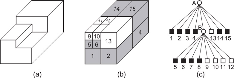
Figure 17.10(a) Example three-dimensional object, (b) its region octree block decomposition, and (c) its tree representation.
The aggregation of cells into blocks in region quadtrees and region octrees is motivated, in part, by a desire to save space. Some of the decompositions have quite a bit of structure thereby leading to inflexibility in choosing partition lines, and so on. In fact, at times, maintaining the original image with an array access structure may be more effective from the standpoint of storage requirements. In the following, we point out some important implications of the use of these aggregations. In particular, we focus on the region quadtree and region octree. Similar results could also be obtained for the remaining block decompositions.
The aggregation of similarly valued cells into blocks has an important effect on the execution time of the algorithms that make use of the region quadtree. In particular, most algorithms that operate on images represented by a region quadtree are implemented by a preorder traversal of the quadtree and, thus, their execution time is generally a linear function of the number of nodes in the quadtree. A key to the analysis of the execution time of quadtree algorithms is the Quadtree Complexity Theorem [47] which states that the number of nodes in a region quadtree representation for a simple polygon (i.e., with nonintersecting edges and without holes) is O(p + q) for a 2q × 2q image with perimeter p measured in terms of the width of unit-sized cells (i.e., pixels). In all but the most pathological cases (e.g., a small square of unit width centered in a large image), the q factor is negligible and thus the number of nodes is O(p).
The Quadtree Complexity Theorem also holds for three-dimensional data [53] (i.e., represented by a region octree) where perimeter is replaced by surface area, as well as for objects of higher dimensions d for which it is proportional to the size of the (d − 1)-dimensional interfaces between these objects. The most important consequence of the Quadtree Complexity Theorem is that it means that most algorithms that execute on a region quadtree representation of an image, instead of one that simply imposes an array access structure on the original collection of cells, usually have an execution time that is proportional to the number of blocks in the image rather than the number of unit-sized cells. Some examples of such algorithms include perimeter computation [54], connected component labeling [55], Euler number [56], and quadtree to raster conversion [57]. Other related ramifications are illustrated by algorithms to compute spatial range queries which related to image dilation (i.e., region expansion and corridor or buffer computation in GIS) [58] which have been observed to execute in time that is independent of the radius of expansion when the regions to be expanded are represented using region quadtrees [59].
In its most general case, the above means that the use of the region quadtree, with an appropriate access structure, in solving a problem in d-dimensional space will lead to a solution whose execution time is proportional to the (d − 1)-dimensional space of the surface of the original d-dimensional image. On the other hand, use of the array access structure on the original collection of cells results in a solution whose execution time is proportional to the number of cells that comprise the image. Therefore, region quadtrees and region octrees act like dimension-reducing devices.
Using a tree access structure captures the characterization of the region quadtree as being of variable resolution in that the underlying space is subdivided recursively until the underlying region satisfies some type of a homogeneity criterion. This is in contrast to a pyramid structure [60,61], which is a family of representations that make use of multiple resolution. This means that the underlying space is subdivided up to the smallest unit (i.e., a pixel) thereby resulting in a complete quadtree, where each leaf node is at the maximum depth and the nonleaf nodes contain information summarizing the contents of their subtrees. The pyramid facilitates feature-based queries [60], which given a feature, identify where it is in space, while the quadtree is more suited for location-based queries, which given a location, identify the features that are associated with it. Feature-based queries have become known as spatial data mining and the pyramid is used to implement them [60,62,63].
The rectangle data type lies somewhere between the point and region data types. It can also be viewed as a special case of the region data type in the sense that it is a region with only four sides. Rectangles are often used to approximate other objects in an image for which they serve as the minimum rectilinear enclosing object. For example, bounding rectangles are used in cartographic applications to approximate objects such as lakes, forests, hills, and so on. In such a case, the approximation gives an indication of the existence of an object. Of course, the exact boundaries of the object are also stored, but they are only accessed if greater precision is needed. For such applications, the number of elements in the collection is usually small, and most often the sizes of the rectangles are of the same order of magnitude as the space from which they are drawn.
Rectangles are also used in VLSI design rule checking as a model of chip components for the analysis of their proper placement. Again, the rectangles serve as minimum enclosing objects. In this application, the size of the collection is quite large (e.g., millions of components) and the sizes of the rectangles are several orders of magnitude smaller than the space from which they are drawn.
It should be clear that the actual representation that is used depends heavily on the problem environment. At times, the rectangle is treated as the Cartesian product of two one-dimensional intervals with the horizontal intervals being treated in a different manner than the vertical intervals. In fact, the representation issue is often reduced to one of representing intervals. For example, this is the case in the use of the plane-sweep paradigm [64] in the solution of rectangle problems such as determining all pairs of intersecting rectangles. In this case, each interval is represented by its left and right endpoints. The solution makes use of two passes.
The first pass sorts the rectangles in ascending order on the basis of their left and right sides (i.e., x coordinate values) and forms a list. The second pass sweeps a vertical scan line through the sorted list from left to right halting at each one of these points, say p. At any instant, all rectangles that intersect the scan line are considered active and are the only ones whose intersection needs to be checked with the rectangle associated with p. This means that each time the sweep line halts, a rectangle either becomes active (causing it to be inserted in the set of active rectangles) or ceases to be active (causing it to be deleted from the set of active rectangles). Thus the key to the algorithm is its ability to keep track of the active rectangles (actually just their vertical sides) as well as to perform the actual one-dimensional intersection test.
Data structures such as the segment tree [65], interval tree [66], and the priority search tree [20] can be used to organize the vertical sides of the active rectangles so that, for N rectangles and F intersecting pairs of rectangles, the problem can be solved in O(N · log2N + F) time. All three data structures enable intersection detection, insertion, and deletion to be executed in O( log2N) time. The difference between them is that the segment tree requires O(N· log2N) space while the interval tree and the priority search tree only need O(N) space. These algorithms require that the set of rectangles be known in advance. However, they work even when the size of the set of active rectangles exceeds the amount of available memory, in which case multiple passes are made over the data [67]. For more details about these data structures, see Chapter 19.
In this chapter, we are primarily interested in dynamic problems (i.e., the set of rectangles is constantly changing). The data structures that are chosen for the collection of the rectangles are differentiated by the way in which each rectangle is represented. One representation discussed in Section 17.1 reduces each rectangle to a point in a higher dimensional space, and then treats the problem as if we have a collection of points [1]. Again, each rectangle is a Cartesian product of two one-dimensional intervals where the difference from its use with the plane-sweep paradigm is that each interval is represented by its centroid and extent. Each set of intervals in a particular dimension is, in turn, represented by a grid file [9] which is described in Section 17.2.
The second representation is region-based in the sense that the subdivision of the space from which the rectangles are drawn depends on the physical extent of the rectangle—not just one point. Representing the collection of rectangles, in turn, with a tree-like data structure has the advantage for some of the representations that there is a relation between the depth of node in the tree and the size of the rectangle(s) that is (are) associated with it. Interestingly, some of the region-based solutions make use of the same data structures that are used in the solutions based on the plane-sweep paradigm.
There are three types of region-based solutions currently in use. The first two solutions use the R-tree and the R+-tree (discussed in Section 17.3) to store rectangle data (in this case the objects are rectangles instead of arbitrary objects). The third is a quadtree-based approach and uses the MX-CIF quadtree [68] (see also Reference 69 for a related variant).
In the MX-CIF quadtree, each rectangle is associated with the quadtree node corresponding to the smallest block which contains it in its entirety. Subdivision ceases whenever a node’s block contains no rectangles. Alternatively, subdivision can also cease once a quadtree block is smaller than a predetermined threshold size. This threshold is often chosen to be equal to the expected size of the rectangle [68]. For example, Figure 17.11b is the MX-CIF quadtree for a collection of rectangles given in Figure 17.11a. Rectangles can be associated with both leaf and nonleaf nodes.

Figure 17.11(a) Collection of rectangles and the block decomposition induced by the MX-CIF quadtree; (b) the tree representation of (a); the binary trees for the y-axes passing through the root of the tree in (b), and (d) the NE son of the root of the tree in (b).
It should be clear that more than one rectangle can be associated with a given enclosing block and, thus, often we find it useful to be able to differentiate between them. This is done in the following manner [68]. Let P be a quadtree node with centroid (CX,CY), and let S be the set of rectangles that are associated with P. Members of S are organized into two sets according to their intersection (or collinearity of their sides) with the lines passing through the centroid of P’s block—that is, all members of S that intersect the line x = CX form one set and all members of S that intersect the line y = CY form the other set.
If a rectangle intersects both lines (i.e., it contains the centroid of P’s block), then we adopt the convention that it is stored with the set associated with the line through x = CX. These subsets are implemented as binary trees (really tries), which in actuality are one-dimensional analogs of the MX-CIF quadtree. For example, Figures 17.11c and d illustrate the binary trees associated with the y-axes passing through the root and the NE son of the root, respectively, of the MX-CIF quadtree of Figure 17.11b. Interestingly, the MX-CIF quadtree is a two-dimensional analog of the interval tree described earlier. More precisely, the MX-CIF quadtree is a two-dimensional analog of the tile tree [70] which is a regular decomposition version of the interval tree. In fact, the tile tree and the one-dimensional MX-CIF quadtree are identical when rectangles are not allowed to overlap.
The drawback of the MX-CIF quadtree is that the size of the minimum enclosing quadtree cells depends on the position of the centroids of the objects and is independent of the size of the objects, subject to a minimum which is the size of the object. In fact, it may be as large as the entire space from which the objects are drawn. This has bad ramifications for applications where the objects move including games, traffic monitoring, and streaming. In particular, if the objects are moved even slightly, then they usually need to be reinserted in the structure.
The cover fieldtree [45,71] and the more commonly known loose quadtree (octree) [72] are designed to overcome this independence of the size of the minimum enclosing quadtree cell and the size of the object (see also the expanded MX-CIF quadtree [73], multiple shifted quadtree methods [74–76], and the partition fieldtree [45,71]). This is done by expanding the size of the space that is spanned by each quadtree cell c of width w by a cell expansion factor p (p > 0) so that the expanded cell is of width (1 + p) · w and an object is associated with its minimum enclosing expanded quadtree (octree) cell. The notion of an expanded quadtree cell can also be seen in the QMAT [43,44]. For example, letting p = 1, Figure 17.12 is the loose quadtree corresponding to the collection of objects in Figure 17.11a and its MX-CIF quadtree in Figure 17.11b. In this example, there are only two differences between the loose and MX-CIF quadtrees:
1.Rectangle object E is associated with the SW child of the root of the loose quadtree instead of with the root of the MX-CIF quadtree.
2.Rectangle object B is associated with the NW child of the NE child of the root of the loose quadtree instead of with the NE child of the root of the MX-CIF quadtree.
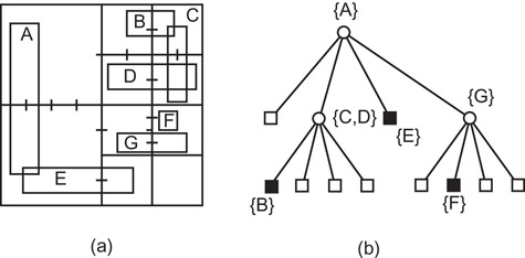
Figure 17.12(a) Cell decomposition induced by the loose quadtree for a collection of rectangle objects identical to those in Figure 17.11 and (b) its tree representation.
Ulrich [72] has shown that given a loose quadtree cell c of width w and cell expansion factor p, the radius r of the minimum bounding hypercube box b of the smallest object o that could possibly be associated with c must be greater than pw/4. Samet et al. [77] point out that the real utility of the loose quadtree is best evaluated in terms of the inverse of the above relation as we are interested in minimizing the maximum possible width w of c given an object o with minimum bounding hypercube box b of radius r (i.e., half the length of a side of the hypercube). This is because reducing w is the real motivation and goal for the development of the loose quadtree as an alternative to the MX-CIF quadtree for which, as we pointed out, w can be as large as the width of the underlying space. This was done by examining the range of the relative widths of c and b as this provides a way of taking into account the constraints imposed by the fact that the range of values of w is limited to powers of 2. In particular, they showed that this range is just a function of p, and hence independent of the position of o. Moreover, they prove that for p ≥ 0.5, the relative widths of c and b take on at most two values, and usually just one value for p ≥ 1. This makes updating the index very simple when objects are moving as there are at most two possible new cells associated with a moved object, instead of log2 of the width of the space in which the objects are embedded (e.g., as large as 16 assuming a 216 × 216 embedding space). In other words, they have shown how to update in O(1) time for p ≥ 0.5 which is of great importance as there is no longer a need to perform a search for the appropriate quadtree cell.
17.6Line Data and Boundaries of Regions
Section 17.4 was devoted to variations on hierarchical decompositions of regions into blocks, an approach to region representation that is based on a description of the region’s interior. In this section, we focus on representations that enable the specification of the boundaries of regions, as well as curvilinear data and collections of line segments. The representations are usually based on a series of approximations which provide successively closer fits to the data, often with the aid of bounding rectangles. When the boundaries or line segments have a constant slope (i.e., linear and termed line segments in the rest of this discussion), then an exact representation is possible.
There are several ways of approximating a curvilinear line segment. The first is by digitizing it and then marking the unit-sized cells (i.e., pixels) through which it passes. The second is to approximate it by a set of straight line segments termed a polyline. Assuming a boundary consisting of straight lines (or polylines after the first stage of approximation), the simplest representation of the boundary of a region is the polygon. It consists of vectors which are usually specified in the form of lists of pairs of x and y coordinate values corresponding to their start and end points. The vectors are usually ordered according to their connectivity. One of the most common representations is the chain code [78] which is an approximation of a polygon’s boundary by use of a sequence of unit vectors in the four (and sometimes eight) principal directions.
Chain codes, and other polygon representations, break down for data in three dimensions and higher. This is primarily due to the difficulty in ordering their boundaries by connectivity. The problem is that in two dimensions connectivity is determined by ordering the boundary elements ei, j of boundary bi of object o so that the end vertex of the vector vj corresponding to ei, j is the start vertex of the vector vj+1 corresponding to ei, j+1. Unfortunately, such an implicit ordering does not exist in higher dimensions as the relationship between the boundary elements associated with a particular object is more complex.
Instead, we must make use of data structures which capture the topology of the object in terms of its faces, edges, and vertices. The winged-edge data structure is one such representation which serves as the basis of the boundary model (also known as BRep [79]). For more details about these data structures, see Chapter 18.
Polygon representations are very local. In particular, if we are at one position on the boundary, we don’t know anything about the rest of the boundary without traversing it element by element. Thus, using such representations, given a random point in space, it is very difficult to find the nearest line to it as the lines are not sorted. This is in contrast to hierarchical representations which are global in nature. They are primarily based on rectangular approximations to the data as well as on a regular decomposition in two dimensions. In the rest of this section, we discuss a number of such representations.
In Section 17.3, we already examined two hierarchical representations (i.e., the R-tree and the R+-tree) that propagate object approximations in the form of bounding rectangles. In this case, the sides of the bounding rectangles had to be parallel to the coordinate axes of the space from which the objects are drawn. In contrast, the strip tree [80] is a hierarchical representation of a single curve that successively approximates segments of it with bounding rectangles that does not require that the sides be parallel to the coordinate axes. The only requirement is that the curve be continuous; it need not be differentiable.
The strip tree data structure consists of a binary tree whose root represents the bounding rectangle of the entire curve. The rectangle associated with the root corresponds to a rectangular strip, that encloses the curve, whose sides are parallel to the line joining the endpoints of the curve. The curve is then partitioned in two at one of the locations where it touches the bounding rectangle (these are not tangent points as the curve only needs to be continuous; it need not be differentiable). Each subcurve is then surrounded by a bounding rectangle and the partitioning process is applied recursively. This process stops when the width of each strip is less than a predetermined value.
In order to be able to cope with more complex curves such as those that arise in the case of object boundaries, the notion of a strip tree must be extended. In particular, closed curves and curves that extend past their endpoints require some special treatment. The general idea is that these curves are enclosed by rectangles which are split into two rectangular strips, and from now on the strip tree is used as before.
The strip tree is similar to the point quadtree in the sense that the points at which the curve is decomposed depend on the data. In contrast, a representation based on the region quadtree has fixed decomposition points. Similarly, strip tree methods approximate curvilinear data with rectangles of arbitrary orientation, while methods based on the region quadtree achieve analogous results by use of a collection of disjoint squares having sides of length power of two. In the following, we discuss a number of adaptations of the region quadtree for representing curvilinear data.
The simplest adaptation of the region quadtree is the MX quadtree [47,81]. It is built by digitizing the line segments and labeling each unit-sized cell (i.e., pixel) through which the line segments pass as of type boundary. The remaining pixels are marked WHITE and are merged, if possible, into larger and larger quadtree blocks. Figure 17.13a is the MX quadtree for the collection of line segment objects in Figure 17.5. A drawback of the MX quadtree is that it associates a thickness with a line. Also, it is difficult to detect the presence of a vertex whenever five or more line segments meet.

Figure 17.13(a) MX quadtree and (b) edge quadtree for the collection of line segments of Figure 17.5.
The edge quadtree [82,83] is a refinement of the MX quadtree based on the observation that the number of squares in the decomposition can be reduced by terminating the subdivision whenever the square contains a single curve that can be approximated by a single straight line. For example, Figure 17.13b is the edge quadtree for the collection of line segment objects in Figure 17.5. Applying this process leads to quadtrees in which long edges are represented by large blocks or a sequence of large blocks. However, small blocks are required in the vicinity of corners or intersecting edges. Of course, many blocks will contain no edge information at all.
The PM quadtree family [39,84] (see also edge-EXCELL [15]) represents an attempt to overcome some of the problems associated with the edge quadtree in the representation of collections of polygons (termed polygonal maps). In particular, the edge quadtree is an approximation because vertices are represented by pixels. There are a number of variants of the PM quadtree. These variants are either vertex-based or edge-based. They are all built by applying the principle of repeatedly breaking up the collection of vertices and edges (forming the polygonal map) until obtaining a subset that is sufficiently simple so that it can be organized by some other data structure.
The PM1 quadtree [39] is an example of a vertex-based PM quadtree. Its decomposition rule stipulates that partitioning occurs as long as a block contains more than one line segment unless the line segments are all incident at the same vertex which is also in the same block (e.g., Figure 17.14a). Given a polygonal map whose vertices are drawn from a grid (say 2m × 2m), and where edges are not permitted to intersect at points other than the grid points (i.e., vertices), it can be shown that the maximum depth of any leaf node in the PM1 quadtree is bounded from above by 4 m + 1 [85]. This enables a determination of the maximum amount of storage that will be necessary for each node. The PM2 quadtree is another vertex-based member of the PM quadtree family that is similar to the PM1 quadtree with the difference that the partitioning of a block b is halted when the line segments in b are all incident at the same vertex v but v need not be in the same block b as is the case for the PM1 quadtree. For example, this means that in the PM2 quadtree there is no need to partition the block corresponding to the NE child of the SW quadrant as in the PM1 quadtree in Figure 17.14a that corresponds to the polygonal map formed by the collection of line segments of Figure 17.5. The PM2 quadtree is particularly useful for polygonal maps that correspond to triangulations where it has been empirically observed to be relatively insensitive to movement of vertices and edges (L. De Floriani, personal communication, 2004).

Figure 17.14(a) PM1 quadtree and (b) PMR quadtree for the collection of line segments of Figure 17.5.
A similar representation to the PM1 quadtree has been devised for polyhedral (i.e., three-dimensional) objects (e.g., see Reference 86 and the references cited in Reference 4). The decomposition criteria are such that no node contains more than one face, edge, or vertex unless the faces all meet at the same vertex or are adjacent to the same edge. This representation is quite useful since its space requirements for polyhedral objects are significantly smaller than those of a region octree.
The PMR quadtree [84] is an edge-based variant of the PM quadtree. It makes use of a probabilistic splitting rule. A node is permitted to contain a variable number of line segments. A line segment is stored in a PMR quadtree by inserting it into the nodes corresponding to all the blocks that it intersects. During this process, the occupancy of each node that is intersected by the line segment is checked to see if the insertion causes it to exceed a predetermined splitting threshold. If the splitting threshold is exceeded, then the node’s block is split once, and only once, into four equal quadrants.
For example, Figure 17.14b is the PMR quadtree for the collection of line segment objects in Figure 17.5 with a splitting threshold value of 2. The line segments are inserted in alphabetic order (i.e., a–i). It should be clear that the shape of the PMR quadtree depends on the order in which the line segments are inserted. Note the difference from the PM1 quadtree in Figure 17.14a—that is, the NE block of the SW quadrant is decomposed in the PM1 quadtree while the SE block of the SW quadrant is not decomposed in the PM1 quadtree.
On the other hand, a line segment is deleted from a PMR quadtree by removing it from the nodes corresponding to all the blocks that it intersects. During this process, the occupancy of the node and its siblings is checked to see if the deletion causes the total number of line segments in them to be less than the predetermined splitting threshold. If the splitting threshold exceeds the occupancy of the node and its siblings, then they are merged and the merging process is reapplied to the resulting node and its siblings. Notice the asymmetry between the splitting and merging rules.
The PMR quadtree is very good for answering queries such as finding the nearest line to a given point [87–90] (see Reference 91 for an empirical comparison with hierarchical object representations such as the R-tree and R+-tree). It is preferred over the PM1 quadtree (as well as the MX and edge quadtrees) as it results in far fewer subdivisions. In particular, in the PMR quadtree there is no need to subdivide in order to separate line segments that are very “close” or whose vertices are very “close,” which is the case for the PM1 quadtree. This is important since four blocks are created at each subdivision step. Thus when many subdivision steps that occur in the PM1 quadtree result in creating many empty blocks, the storage requirements of the PM1 quadtree will be considerably higher than those of the PMR quadtree. Generally, as the splitting threshold is increased, the storage requirements of the PMR quadtree decrease while the time necessary to perform operations on it will increase.
Using a random image model and geometric probability, it has been shown [92], theoretically and empirically using both random and real map data, that for sufficiently high values of the splitting threshold (i.e., ≥4), the number of nodes in a PMR quadtree is asymptotically proportional to the number of line segments and is independent of the maximum depth of the tree. In contrast, using the same model, the number of nodes in the PM1 quadtree is a product of the number of lines and the maximal depth of the tree (i.e., n for a 2n × 2n image). The same experiments and analysis for the MX quadtree confirmed the results predicted by the Quadtree Complexity Theorem (see Section 17.4) which is that the number of nodes is proportional to the total length of the line segments. Observe that although a bucket in the PMR quadtree can contain more line segments than the splitting threshold, this is not a problem. In fact, it can be shown [4] that the maximum number of line segments in a bucket is bounded by the sum of the splitting threshold and the depth of the block (i.e., the number of times the original space has been decomposed to yield this block).
When the line segments that make up the polygonal map are orthogonal and parallel to the coordinate axes, then we can make use of the line quadtree [93,94] which is an enhancement of the region quadtree where the boundaries of the regions are coincident with the quadtree blocks and are also represented in a hierarchical manner. In particular, the line quadtree recursively partitions the underlying space until obtaining blocks (possibly single pixels) that have no boundary elements passing through their interior. Associated with each block is a four bit code which indicates which of its four sides forms a boundary (not a partial boundary) of any single object (including the underlying space). Thus instead of distinguishing blocks on the basis of whether they are part of the background, and of the identity of the object in which they lie, we use the nature of the boundary information. Note the distinction from the region quadtree where no information is associated with the nonleaf nodes. In this respect, it is more like the pyramid (see Section 17.4).
17.7Research Issues and Summary
A review has been presented of a number of representations of multidimensional data. Our focus has been on multidimensional spatial data with extent rather than just multidimensional point data. There has been a particular emphasis on hierarchical representations. Such representations are based on the “divide-and-conquer” problem-solving paradigm. They are of interest because they enable focusing computational resources on the interesting subsets of data. Thus there is no need to expend work where the payoff is small. Although many of the operations for which they are used can often be performed equally as efficiently, or more so, with other data structures, hierarchical data structures are attractive because of their conceptual clarity and ease of implementation.
When the hierarchical data structures are based on the principle of regular decomposition, we have the added benefit that different data sets (often of differing types) are in registration. This means that they are partitioned in known positions which are often the same or subsets of one another for the different data sets. This is true for all the features including regions, points, rectangles, lines, volumes, and so on. The result is that a query such as “finding all cities with more than 20,000 inhabitants in wheat-growing regions within 30 miles of the Mississippi River” can be executed by simply overlaying the region (crops), point (i.e., cities), and river maps even though they represent data of different types. Alternatively, we may extract regions such as those within 30 miles of the Mississippi River. Such operations find use in applications involving spatial data such as GIS.
Current research in multidimensional representations is highly application dependent in the sense that the work is driven by the application. Many of the recent developments have been motivated by the interaction with databases. This is facilitated by the existence of browsing (e.g., [95–98]) or manipulating (e.g., by what is termed a spatial spreadsheet [99]) capabilities. The choice of a proper representation plays a key role in the speed with which responses are provided to queries. Knowledge of the underlying data distribution is also a factor and research is ongoing to make use of this information in the process of making a choice. Most of the initial applications in which the representation of multidimensional data has been important have involved spatial data of the kind described in this chapter. Such data is intrinsically of low dimensionality (i.e., two and three).
Future applications involve higher dimensional data for applications such as image databases where the data are often points in feature space. Unfortunately, for such applications, the performance of most indexing methods that rely on a decomposition of the underlying space is often unsatisfactory when compared with not using an index at all [100]. The problem is that for uniformly distributed data, most of the data is found to be at or near the boundary of the space in which it lies [101]. The result means that the query region usually overlaps all of the leaf node regions that are created by the decomposition process and thus a sequential scan is preferable. This has led to a number of alternative representations that try to speed up the scan (e.g., VA-file [102], VA+-file [103], IQ-tree [104], etc.). Nevertheless, representations such as the pyramid technique [105] are based on the principle that most of the data lies near the surface and therefore subdivide the data space as if it is an onion by peeling off hypervolumes that are close to its boundary. This is achieved by first dividing the hypercube corresponding to the d-dimensional data space into 2d pyramids having the center of the data space as their top point and one of the faces of the hypercube as its base. These pyramids are subsequently cut into slices that are parallel to their base. Of course, the high-dimensional data is not necessarily uniformly distributed which has led to other data structures with good performance (e.g., the hybrid tree [106]). Clearly, more work needs to be done in this area.
It is interesting to observe that the rise of the use of the world wide web has made spatial multidimensional data such as locations much more common. The explicit specification of location has traditionally been geometric (e.g., as latitude–longitude pairs of numbers). Unfortunately, this is not easy as most people don’t usually know of a location in this way. Even more important is the fact that they don’t know where to obtain this information and are not used to communicate or receive it from others in this way. Instead, they are used to specify a location textually which includes verbally.
The principal drawback of the textual specification of location data is that it is potentially ambiguous. First of all, we must be sure that the textual entity actually corresponds to a location (termed a toponym) rather than the name of a person, an organization, or an object, to name a few of many possible alternative interpretations. The process of determining whether a textual entity is a toponym is termed toponym recognition [107]. Moreover, having identified the textual entity as a toponym such as “Alexandria,” there are many possible locations named “Alexandria” and they must be resolved. This process is known as toponym resolution [108,109]. Moreover, in some cases we are not even sure that the term “Lincoln” denotes a location as it could be a reference to the name of a person. Both of these issues can arise when processing documents such as newspaper articles [110–114], tweets [115–117], blogs, and so on. The process of understanding and converting location text to its geometric specification, known as geotagging [118–126], serves as a prerequisite to indexing the data and is the subject of much research.
This work was supported, in part, by the National Science Foundation under grants IRI-97-12715, EIA-99-00268, IIS-00-86162, EIA-00-91474, IIS-12-19023, and IIS-13-20791.
1.K. Hinrichs and J. Nievergelt. The grid file: A data structure designed to support proximity queries on spatial objects. In Proceedings of WG’83, International Workshop on Graphheoretic Concepts in Computer Science, M. Nagl and J. Perl, eds., pages 100–113, Trauner Verlag, Haus Ohrbeck (near Osnabrück), West Germany, 1983.
2.J.-W. Song, K.-Y. Whang, Y.-K. Lee, M.-J. Lee, and S.-W. Kim. Spatial join processing using corner transformation. IEEE Transactions on Knowledge and Data Engineering, 11(4):688–695, July/August 1999.
3.H. Samet. Applications of Spatial Data Structures: Computer Graphics, Image Processing, and GIS. Addison-Wesley, Reading, MA, 1990.
4.H. Samet. The Design and Analysis of Spatial Data Structures. Addison-Wesley, Reading, MA, 1990.
5.H. Samet. Foundations of Multidimensional and Metric Data Structures. Morgan-Kaufmann, San Francisco, 2006. (Translated to Chinese ISBN 978-7-302-22784-7).
6.D. E. Knuth. Big omicron and big omega and big theta. SIGACT News, 8(2):18–24, April–June 1976.
7.D. E. Knuth. The Art of Computer Programming: Sorting and Searching, vol. 3. Addison-Wesley, Reading, MA, 1973.
8.J. L. Bentley and J. H. Friedman. Data structures for range searching. ACM Computing Surveys, 11(4):397–409, December 1979.
9.J. Nievergelt, H. Hinterberger, and K. C. Sevcik. The grid file: An adaptable, symmetric multikey file structure. ACM Transactions on Database Systems, 9(1):38–71, March 1984.
10.J. L. Bentley, D. F. Stanat, and E. H. Williams, Jr. The complexity of finding fixed-radius near neighbors. Information Processing Letters, 6(6):209–212, December 1977.
11.R. A. Finkel and J. L. Bentley. Quad trees: A data structure for retrieval on composite keys. Acta Informatica, 4(1):1–9, 1974.
12.J. A. Orenstein. Multidimensional tries used for associative searching. Information Processing Letters, 14(4):150–157, June 1982.
13.E. Fredkin. Trie memory. Communications of the ACM, 3(9):490–499, September 1960.
14.J. L. Bentley. Multidimensional binary search trees used for associative searching. Communications of the ACM, 18(9):509–517, September 1975.
15.M. Tamminen. The EXCELL method for efficient geometric access to data. Series Acta Polytechnica Scandinavica, 1981. Also Mathematics and Computer Science Series No. 34.
16.D. Comer. The ubiquitous B-tree. ACM Computing Surveys, 11(2):121–137, June 1979.
17.H. Samet. Decoupling: A spatial indexing solution. Computer Science Technical Report TR-4523, University of Maryland, College Park, MD, August 2003.
18.W. Wang, J. Yang, and R. Muntz. PK-tree: A spatial index structure for high dimensional point data. In Proceedings of the 5th International Conference on Foundations of Data Organization and Algorithms (FODO), K. Tanaka and S. Ghandeharizadeh, eds., pages 27–36, Kobe, Japan, November 1998. Also University of California at Los Angeles Computer Science Technical Report 980032, September 1998.
19.J. L. Bentley and H. A. Maurer. Efficient worst-case data structures for range searching. Acta Informatica, 13:155–168, 1980.
20.E. M. McCreight. Priority search trees. SIAM Journal on Computing, 14(2):257–276, May 1985. Also Xerox Palo Alto Research Center Technical Report CSL-81-5, January 1982.
21.N. Beckmann, H.-P. Kriegel, R. Schneider, and B. Seeger. The R*-tree: An efficient and robust access method for points and rectangles. In Proceedings of the ACM SIGMOD Conference, pages 322–331, Atlantic City, NJ, June 1990.
22.A. Guttman. R-trees: A dynamic index structure for spatial searching. In Proceedings of the ACM SIGMOD Conference, pages 47–57, Boston, June 1984.
23.D. A. White and R. Jain. Similarity indexing with the SS-tree. In Proceedings of the 12th IEEE International Conference on Data Engineering, S. Y. W. Su, ed., pages 516–523, New Orleans, LA, February 1996.
24.N. Katayama and S. Satoh. The SR-tree: An index structure for high-dimensional nearest neighbor queries. In Proceedings of the ACM SIGMOD Conference, J. Peckham, ed., pages 369–380, Tucson, AZ, May 1997.
25.S. Gottschalk, M. C. Lin, and D. Manocha. OBBTree: A hierarchical structure for rapid interference detection. In Proceedings of the SIGGRAPH’96 Conference, pages 171–180, New Orleans, LA, August 1996.
26.R. Bayer and E. M. McCreight. Organization and maintenance of large ordered indexes. Acta Informatica, 1(3):173–189, 1972.
27.W. G. Aref and H. Samet. Uniquely reporting spatial objects: Yet another operation for comparing spatial data structures. In Proceedings of the 5th International Symposium on Spatial Data Handling, pages 178–189, Charleston, SC, August 1992.
28.W. G. Aref and H. Samet. Hashing by proximity to process duplicates in spatial databases. In Proceedings of the 3rd International Conference on Information and Knowledge Management (CIKM), pages 347–354, Gaithersburg, MD, December 1994.
29.J.-P. Dittrich and B. Seeger. Data redundancy and duplicate detection in spatial join processing. In Proceedings of the 16th IEEE International Conference on Data Engineering, pages 535–546, San Diego, CA, February 2000.
30.J. T. Robinson. The K-D-B-tree: A search structure for large multidimensional dynamic indexes. In Proceedings of the ACM SIGMOD Conference, pages 10–18, Ann Arbor, MI, April 1981.
31.T. Sellis, N. Roussopoulos, and C. Faloutsos. The R+-tree: A dynamic index for multi-dimensional objects. In Proceedings of the 13th International Conference on Very Large Databases (VLDB), P. M. Stocker and W. Kent, eds., pages 71–79, Brighton, UK, September 1987. Also University of Maryland Computer Science Technical Report TR-1795, 1987.
32.M. Stonebraker, T. Sellis, and E. Hanson. An analysis of rule indexing implementations in data base systems. In Proceedings of the 1st International Conference on Expert Database Systems, pages 353–364, Charleston, SC, April 1986.
33.O. Günther. Efficient structures for geometric data management. PhD thesis, Computer Science Division, University of California at Berkeley, Berkeley, CA, 1987. Also vol. 37 of Lecture Notes in Computer Science, Springer-Verlag, Berlin, West Germany, 1988 and Electronics Research Laboratory Memorandum UCB/ERL M87/77.
34.A. Henrich, H.-W. Six, and P. Widmayer. The LSD tree: Spatial access to multidimensional point and non-point data. In Proceedings of the 15th International Conference on Very Large Databases (VLDB), P. M. G. Apers and G. Wiederhold, eds., pages 45–53, Amsterdam, The Netherlands, August 1989.
35.D. Lomet and B. Salzberg. The hB-tree: A multi-attribute indexing method with good guaranteed performance. ACM Transactions on Database Systems, 15(4):625–658, December 1990. Also see Proceedings of the 5th IEEE International Conference on Data Engineering, pages 296–304, Los Angeles, February 1989 and Northeastern University Computer Science Technical Report NU-CCS-87-24, 1987.
36.M. Freeston. The BANG file: A new kind of grid file. In Proceedings of the ACM SIGMOD Conference, pages 260–269, San Francisco, May 1987.
37.M. Freeston. A general solution of the n-dimensional B-tree problem. In Proceedings of the ACM SIGMOD Conference, pages 80–91, San Jose, CA, May 1995.
38.W. R. Franklin. Adaptive grids for geometric operations. Cartographica, 21(2&3):160–167, Summer & Autumn 1984.
39.H. Samet and R. E. Webber. Storing a collection of polygons using quadtrees. ACM Transactions on Graphics, 4(3):182–222, July 1985. Also see Proceedings of Computer Vision and Pattern Recognition’83, pages 127–132, Washington, DC, June 1983 and University of Maryland Computer Science Technical Report TR-1372, February 1984.
40.A. A. G. Requicha. Representations of rigid solids: Theory, methods, and systems. ACM Computing Surveys, 12(4):437–464, December 1980.
41.H. Samet and M. Tamminen. Bintrees, CSG trees, and time. Computer Graphics, 19(3):121–130, July 1985. Also in Proceedings of the SIGGRAPH’85 Conference, San Francisco, July 1985.
42.H. Samet and M. Tamminen. Approximating CSG trees of moving objects. Visual Computer, 6(4):182–209, August 1990. Also University of Maryland Computer Science Technical Report TR-1472, January 1985.
43.H. Samet. A quadtree medial axis transform. Communications of the ACM, 26(9):680–693, September 1983. Also see CORRIGENDUM, Communications of the ACM, 27(2):151, February 1984 and University of Maryland Computer Science Technical Report TR-803, August 1979.
44.H. Samet. Reconstruction of quadtrees from quadtree medial axis transforms. Computer Vision, Graphics, and Image Processing, 29(3):311–328, March 1985. Also University of Maryland Computer Science Technical Report TR-1224, October 1982.
45.A. U. Frank and R. Barrera. The Fieldtree: A data structure for geographic information systems. In Design and Implementation of Large Spatial Databases—1st Symposium, SSD’89, A. Buchmann, O. Günther, T. R. Smith, and Y.-F. Wang, eds., vol. 409 of Springer-Verlag Lecture Notes in Computer Science, pages 29–44, Santa Barbara, CA, July 1989.
46.A. Klinger. Patterns and search statistics. In Optimizing Methods in Statistics, J. S. Rustagi, ed., pages 303–337. Academic Press, New York, 1971.
47.G. M. Hunter. Efficient computation and data structures for graphics. PhD thesis, Department of Electrical Engineering and Computer Science, Princeton University, Princeton, NJ, 1978.
48.D. Meagher. Geometric modeling using octree encoding. Computer Graphics and Image Processing, 19(2):129–147, June 1982.
49.K. Knowlton. Progressive transmission of grey-scale and binary pictures by simple efficient, and lossless encoding schemes. Proceedings of the IEEE, 68(7):885–896, July 1980.
50.H. Samet and M. Tamminen. Efficient component labeling of images of arbitrary dimension represented by linear bintrees. IEEE Transactions on Pattern Analysis and Machine Intelligence, 10(4):579–586, July 1988.
51.M. Tamminen. Comment on quad- and octrees. Communications of the ACM, 27(3):248–249, March 1984.
52.H. Fuchs, Z. M. Kedem, and B. F. Naylor. On visible surface generation by a priori tree structures. Computer Graphics, 14(3):124–133, July 1980. Also in Proceedings of the SIGGRAPH’80 Conference, Seattle, WA, July 1980.
53.D. Meagher. Octree encoding: A new technique for the representation, manipulation, and display of arbitrary 3-D objects by computer. Electrical and Systems Engineering Technical Report IPL-TR-80-111, Rensselaer Polytechnic Institute, Troy, NY, October 1980.
54.H. Samet. Computing perimeters of images represented by quadtrees. IEEE Transactions on Pattern Analysis and Machine Intelligence, 3(6):683–687, November 1981. Also University of Maryland Computer Science Technical Report TR-755, April 1979.
55.H. Samet and M. Tamminen. An improved approach to connected component labeling of images. In Proceedings of Computer Vision and Pattern Recognition’86, pages 312–318, Miami Beach, FL, June 1986. Also see University of Maryland Computer Science Technical Report TR-1649, August 1986.
56.C. R. Dyer. Computing the Euler number of an image from its quadtree. Computer Graphics and Image Processing, 13(3):270–276, July 1980. Also University of Maryland Computer Science Technical Report TR-769, May 1979.
57.H. Samet. Algorithms for the conversion of quadtrees to rasters. Computer Vision, Graphics, and Image Processing, 26(1):1–16, April 1984. Also University of Maryland Computer Science Technical Report TR-979, November 1980.
58.A. Amir, A. Efrat, P. Indyk, and H. Samet. Efficient algorithms and regular data structures for dilation, location and proximity problems. Algorithmica, 30(2):164–187, 2001. Also see Proceedings of the 40th IEEE Annual Symposium on Foundations of Computer Science, pages 160–170, New York, October 1999 and University of Maryland Computer Science Technical Report TR-4201, November 2000.
59.C.-H. Ang, H. Samet, and C. A. Shaffer. A new region expansion for quadtrees. IEEE Transactions on Pattern Analysis and Machine Intelligence, 12(7):682–686, July 1990. Also see Proceedings of the Third International Symposium on Spatial Data Handling, pages 19–37, Sydney, Australia, August 1988.
60.W. G. Aref and H. Samet. Efficient processing of window queries in the pyramid data structure. In Proceedings of the 9th ACM SIGACT–SIGMOD–SIGART Symposium on Principles of Database Systems (PODS), pages 265–272, Nashville, TN, April 1990. Also in Proceedings of the Fifth Brazilian Symposium on Databases, pages 15–26, Rio de Janeiro, Brazil, April 1990.
61.S. L. Tanimoto and T. Pavlidis. A hierarchical data structure for picture processing. Computer Graphics and Image Processing, 4(2):104–119, June 1975.
62.J. Han and M. Kamber. Data Mining: Concepts and Techniques. Morgan Kaufmann, San Francisco, 2000.
63.W. Wang, J. Yang, and R. R. Muntz. STING: A statistical information grid approach to spatial data mining. In Proceedings of the 23rd International Conference on Very Large Data Bases (VLDB), M. Jarke, M. J. Carey, K. R. Dittrich, F. H. Lochovsky, P. Loucopoulos, and M. A. Jeusfeld, eds., pages 186–195, Athens, Greece, August 1997.
64.F. P. Preparata and M. I. Shamos. Computational Geometry: An Introduction. Springer-Verlag, New York, 1985.
65.J. L. Bentley. Algorithms for Klee’s Rectangle Problems (Unpublished). Computer Science Department, Carnegie-Mellon University, Pittsburgh, PA, 1977.
66.H. Edelsbrunner. Dynamic rectangle intersection searching. Institute for Information Processing Technical Report 47, Technical University of Graz, Graz, Austria, February 1980.
67.E. Jacox and H. Samet. Iterative spatial join. ACM Transactions on Database Systems, 28(3):268–294, September 2003.
68.G. Kedem. The quad-CIF tree: A data structure for hierarchical on-line algorithms. In Proceedings of the 19th Design Automation Conference, pages 352–357, Las Vegas, NV, June 1982. Also University of Rochester Computer Science Technical Report TR-91, September 1981.
69.G. G. Lai, D. Fussell, and D. F. Wong. HV/VH trees: A new spatial data structure for fast region queries. In Proceedings of the 30th ACM/IEEE Design Automation Conference, pages 43–47, Dallas, TX, June 1993.
70.E. M. McCreight. Efficient algorithms for enumerating intersecting intervals and rectangles. Technical Report CSL-80-09, Xerox Palo Alto Research Center, Palo Alto, CA, June 1980.
71.A. Frank. Problems of realizing LIS: Storage methods for space related data: The fieldtree. Technical Report 71, Institute for Geodesy and Photogrammetry, ETH, Zurich, Switzerland, June 1983.
72.T. Ulrich. Loose octrees. In Game Programming Gems, M. A. DeLoura, ed., pages 444–453. Charles River Media, Rockland, MA, 2000.
73.D. J. Abel and J. L. Smith. A data structure and query algorithm for a database of areal entities. Australian Computer Journal, 16(4):147–154, November 1984.
74.T. M. Chan. Approximate nearest neighbor queries revisited. In Proceedings of the 13th Annual Symposium on Computational Geometry, pages 352–358, Nice, France, June 1997.
75.S. Liao, M. A. Lopez, and S. T. Leutenegger. High dimensional similarity search with space filling curves. In Proceedings of the 17th IEEE International Conference on Data Engineering, pages 615–622, Heidelberg, Germany, April 2001.
76.M. D. Lieberman, J. Sankaranarayanan, and H. Samet. A fast similarity join algorithm using graphics processing units. In Proceedings of the 24th IEEE International Conference on Data Engineering, pages 1111–1120, Cancun, Mexico, April 2008.
77.H. Samet, J. Sankaranarayanan, and M. Auerbach. Indexing methods for moving object databases: Games and other applications. In Proceedings of the ACM SIGMOD Conference, pages 169–180, New York, June 2013.
78.H. Freeman. Computer processing of line-drawing images. ACM Computing Surveys, 6(1):57–97, March 1974.
79.B. G. Baumgart. A polyhedron representation for computer vision. In Proceedings of the 1975 National Computer Conference, vol. 44, pages 589–596, Anaheim, CA, May 1975.
80.D. H. Ballard. Strip trees: A hierarchical representation for curves. Communications of the ACM, 24(5):310–321, May 1981. Also see corrigendum, Communications of the ACM, 25(3):213, March 1982.
81.G. M. Hunter and K. Steiglitz. Operations on images using quad trees. IEEE Transactions on Pattern Analysis and Machine Intelligence, 1(2):145–153, April 1979.
82.M. Shneier. Two hierarchical linear feature representations: Edge pyramids and edge quadtrees. Computer Graphics and Image Processing, 17(3):211–224, November 1981. Also University of Maryland Computer Science Technical Report TR-961, October 1980.
83.J. E. Warnock. A hidden surface algorithm for computer generated half tone pictures. Computer Science Technical Report TR 4–15, University of Utah, Salt Lake City, UT, June 1969.
84.R. C. Nelson and H. Samet. A consistent hierarchical representation for vector data. Computer Graphics, 20(4):197–206, August 1986. Also in Proceedings of the SIGGRAPH’86 Conference, Dallas, TX, August 1986.
85.H. Samet, C. A. Shaffer, and R. E. Webber. Digitizing the plane with cells of non-uniform size. Information Processing Letters, 24(6):369–375, April 1987. Also an expanded version in University of Maryland Computer Science Technical Report TR-1619, January 1986.
86.D. Ayala, P. Brunet, R. Juan, and I. Navazo. Object representation by means of nonminimal division quadtrees and octrees. ACM Transactions on Graphics, 4(1):41–59, January 1985.
87.G. R. Hjaltason and H. Samet. Ranking in spatial databases. In Advances in Spatial Databases—4th International Symposium, SSD’95, M. J. Egenhofer and J. R. Herring, eds., vol. 951 of Springer-Verlag Lecture Notes in Computer Science, pages 83–95, Portland, ME, August 1995.
88.G. R. Hjaltason and H. Samet. Distance browsing in spatial databases. ACM Transactions on Database Systems, 24(2):265–318, June 1999. Also University of Maryland Computer Science Technical Report TR-3919, July 1998.
89.G. R. Hjaltason and H. Samet. Index-driven similarity search in metric spaces. ACM Transactions on Database Systems, 28(4):517–580, December 2003.
90.E. G. Hoel and H. Samet. Efficient processing of spatial queries in line segment databases. In Advances in Spatial Databases—2nd Symposium, SSD’91, O. Günther and H.-J. Schek, eds., vol. 525 of Springer-Verlag Lecture Notes in Computer Science, pages 237–256, Zurich, Switzerland, August 1991.
91.E. G. Hoel and H. Samet. A qualitative comparison study of data structures for large line segment databases. In Proceedings of the ACM SIGMOD Conference, M. Stonebraker, ed., pages 205–214, San Diego, CA, June 1992.
92.M. Lindenbaum and H. Samet. A probabilistic analysis of trie-based sorting of large collections of line segments. Computer Science Technical Report TR-3455, University of Maryland, College Park, MD, April 1995. Also an expanded version in SIAM Journal on Computing, 35(1):22–58, September 2005 and TR-3455.1, February 2000.
93.H. Samet and R. E. Webber. On encoding boundaries with quadtrees. Computer Science Technical Report TR-1162, University of Maryland, College Park, MD, February 1982.
94.H. Samet and R. E. Webber. On encoding boundaries with quadtrees. IEEE Transactions on Pattern Analysis and Machine Intelligence, 6(3):365–369, May 1984.
95.C. Esperança and H. Samet. Experience with SAND/Tcl: A scripting tool for spatial databases. Journal of Visual Languages and Computing, 13(2):229–255, April 2002.
96.H. Samet, H. Alborzi, F. Brabec, C. Esperança, G. R. Hjaltason, F. Morgan, and E. Tanin. Use of the SAND spatial browser for digital government applications. Communications of the ACM, 46(1):63–66, January 2003.
97.H. Samet, A. Rosenfeld, C. A. Shaffer, and R. E. Webber. A geographic information system using quadtrees. Pattern Recognition, 17(6):647–656, November/December 1984.
98.C. A. Shaffer, H. Samet, R. C. Nelson. QUILT: A geographic information system based on quadtrees. International Journal of Geographical Information Systems, 4(2):103–131, April–June 1990. Also University of Maryland Computer Science Technical Report TR-1885.1, July 1987.
99.G. S. Iwerks and H. Samet. The spatial spreadsheet. In Proceedings of the 3rd International Conference on Visual Information Systems (VISUAL99), D. P. Huijsmans and A. W. M. Smeulders, eds., pages 317–324, Amsterdam, The Netherlands, June 1999.
100.K. S. Beyer, J. Goldstein, R. Ramakrishnan, and U. Shaft. When is “nearest neighbor” meaningful? In Proceedings of the 7th International Conference on Database Theory (ICDT’99), C. Beeri and P. Buneman, eds., vol. 1540 of Springer-Verlag Lecture Notes in Computer Science, pages 217–235, Berlin, Germany, January 1999.
101.S. Berchtold, C. Böhm, and H.-P. Kriegel. Improving the query performance of high-dimensional index structures by bulk-load operations. In Advances in Database Technology—EDBT’98, Proceedings of the 6th International Conference on Extending Database Technology, H.-J Schek, F. Saltor, I. Ramos, and G. Alonso, eds., vol. 1377 of Springer-Verlag Lecture Notes in Computer Science, pages 216–230, Valencia, Spain, March 1998.
102.R. Weber, H.-J. Schek, and S. Blott. A quantitative analysis and performance study for similarity-search methods in high-dimensional spaces. In Proceedings of the 24th International Conference on Very Large Data Bases (VLDB), A. Gupta, O. Shmueli, and J. Widom, eds., pages 194–205, New York, August 1998.
103.H. Ferhatosmanoglu, E. Tuncel, D. Agrawal, and A. El Abbadi. Vector approximation based indexing for non-uniform high dimensional data sets. In Proceedings of the 9th International Conference on Information and Knowledge Management (CIKM), pages 202–209, McLean, VA, November 2000.
104.S. Berchtold, C. Böhm, H. V. Jagadish, H.-P. Kriegel, and J. Sander. Independent quantization: An index compression technique for high-dimensional data spaces. In Proceedings of the 16th IEEE International Conference on Data Engineering, pages 577–588, San Diego, CA, February 2000.
105.S. Berchtold, C. Böhm, and H.-P. Kriegel. The pyramid-technique: Towards breaking the curse of dimensionality. In Proceedings of the ACM SIGMOD Conference, L. Hass and A. Tiwary, eds., pages 142–153, Seattle, WA, June 1998.
106.K. Chakrabarti and S. Mehrotra. The hybrid tree: An index structure for high dimensional feature spaces. In Proceedings of the 15th IEEE International Conference on Data Engineering, pages 440–447, Sydney, Australia, March 1999. Also University of California at Irvine Information and Computer Science Technical Report TR-MARS-98-14, July 1998.
107.M. D. Lieberman and H. Samet. Multifaceted toponym recognition for streaming news. In Proceedings of the 34th International Conference on Research and Development in Information Retrieval (SIGIR’11), pages 843–852, Beijing, China, July 2011.
108.M. D. Lieberman and H. Samet. Adaptive context features for toponym resolution in streaming news. In Proceedings of the 35th International Conference on Research and Development in Information Retrieval (SIGIR’12), pages 731–740, Portland, OR, August 2012.
109.H. Samet. Using minimaps to enable toponym resolution with an effective 100% rate of recall. In Proceedings of 8th ACM SIGSPATIAL Workshop on Geographic Information Retrieval (GIR’14), R. Purves and C. Jones, eds., pages 9:1–9:8, Dallas, TX, November 2014.
110.M. D. Lieberman and H. Samet. Supporting rapid processing and interactive map-based exploration of streaming news. In Proceedings of the 20th ACM SIGSPATIAL International Conference on Advances in Geographic Information Systems, I. Cruz, C. A. Knoblock, P. Kröger, E. Tanin, and P. Widmayer, eds., pages 179–188, Redondo Beach, CA, November 2012.
111.H. Samet, M. D. Adelfio, B. C. Fruin, M. D. Lieberman, and B. E. Teitler. Porting a web-based mapping application to a smartphone app. In Proceedings of the 19th ACM SIGSPATIAL International Conference on Advances in Geographic Information Systems, D. Agrawal, I. Cruz, C. S. Jensen, E. Ofek, and E. Tanin, eds., pages 525–528, Chicago, November 2011.
112.H. Samet, J. Sankaranarayanan, M. D. Lieberman, M. D. Adelfio, B. C. Fruin, J. M. Lotkowski, D. Panozzo, J. Sperling, and B. E. Teitler. Reading news with maps by exploiting spatial synonyms. Communications of the ACM, 57(10):64–77, October 2014.
113.H. Samet, B. E. Teitler, M. D. Adelfio, and M. D. Lieberman. Adapting a map query interface for a gesturing touch screen interface. In Proceedings of the Twentieth International Word Wide Web Conference (Companion Volume), S. Srinivasan, K. Ramamritham, A. Kumar, M. P. Ravindra, E. Bertino, and R. Kumar, eds., pages 257–260, Hyderabad, India, March-April 2011.
114.B. Teitler, M. D. Lieberman, D. Panozzo, J. Sankaranarayanan, H. Samet, and J. Sperling. News Stand: A new view on news. In Proceedings of the 16th ACM SIGSPATIAL International Conference on Advances in Geographic Information Systems, W. G. Aref, M. F. Mokbel, H. Samet, M. Schneider, C. Shahabi, and O. Wolfson, eds., pages 144–153, Irvine, CA, November 2008.
115.N. Gramsky and H. Samet. Seeder finder—Identifying additional needles in the Twitter haystack. In Proceedings of the 6th ACM SIGSPATIAL International Workshop on Location-Based Social Networks (LBSN’13), A. Pozdnukhov, ed., pages 44–53, Orlando, FL, November 2013.
116.A. Jackoway, H. Samet, and J. Sankaranarayanan. Identification of live news events using Twitter. In Proceedings of the 3rd ACM SIGSPATIAL International Workshop on Location-Based Social Networks (LBSN’11), Y. Zheng and M. F. Mokbel, eds., pages 25–32, Chicago, November 2011.
117.J. Sankaranarayanan, H. Samet, B. Teitler, M. D. Lieberman, and J. Sperling. TwitterStand: News in tweets. In Proceedings of the 17th ACM SIGSPATIAL International Conference on Advances in Geographic Information Systems, D. Agrawal, W. G. Aref, C.-T. Lu, M. F. Mokbel, P. Scheuermann, C. Shahabi, and O. Wolfson, eds., pages 42–51, Seattle, WA, November 2009.
118.M. D. Adelfio and H. Samet. Structured toponym resolution using combined hierarchical place categories. In Proceedings of 7th ACM SIGSPATIAL Workshop on Geographic Information Retrieval (GIR’13), R. Purves and C. Jones, eds., pages 49–56, Orlando, FL, November 2013.
119.E. Amitay, N. Har’El, R. Sivan, and A. Soffer. Web-a-Where: Geotagging web content. In Proceedings of the 27th International Conference on Research and Development in Information Retrieval (SIGIR’04), M. Sanderson, K. Järvelin, J. Allan, and P. Bruza, eds., pages 273–280, Sheffield, UK, July 2004.
120.C. B. Jones, R. S. Purves, P. D. Clough, and H. Joho. Modelling vague places with knowledge from the Web. International Journal of Geographical Information Systems, 22(10):1045–1065, 2008.
121.J. L. Leidner and M. D. Lieberman. Detecting geographical references in the form of place names and associated spatial natural language. SIGSPATIAL Special, 3(2):5–11, 2011.
122.M. D. Lieberman, H. Samet, and J. Sankaranarayanan. Geotagging: Using proximity, sibling, and prominence clues to understand comma groups. In Proceedings of 6th Workshop on Geographic Information Retrieval, R. Purves, C. Jones, and P. Clough, eds., Zurich, Switzerland, February 2010. Article 6.
123.M. D. Lieberman, H. Samet, and J. Sankaranarayanan. Geotagging with local lexicons to build indexes for textually-specified spatial data. In Proceedings of the 26th IEEE International Conference on Data Engineering, pages 201–212, Long Beach, CA, March 2010.
124.B. Martins, H. Manguinhas, and J. Borbinha. Extracting and exploring the geo-temporal semantics of textual resources. In Proceedings of the 2th IEEE International Conference on Semantic Computing (ICSC’08), pages 1–9, Santa Clara, CA, August 2008.
125.R. S. Purves, P. Clough, C. B. Jones, A. Arampatzis, B. Bucher, D. Finch, G. Fu, H. Joho, A. K Syed, S. Vaid, and B. Yang. The design and implementation of SPIRIT: A spatially aware search engine for information retrieval on the internet. International Journal of Geographical Information Systems, 21(7):717–745, 2007.
126.G. Quercini, H. Samet, J. Sankaranarayanan, and M. D. Lieberman. Determining the spatial reader scopes of news sources using local lexicons. In Proceedings of the 18th ACM SIGSPATIAL International Conference on Advances in Geographic Information Systems, A. El Abbadi, D. Agrawal, M. Mokbel, and P. Zhang, eds., pages 43–52, San Jose, CA, November 2010.
*All figures © 2017 by Hanan Samet.
*From a theoretical viewpoint, the bounding rectangles for the objects at the leaf nodes should also be disjoint. However, this may be impossible (e.g., when the objects are line segments and if many of the line segments intersect at a point).
*A (linear) half-space in d-dimensional space is defined by the inequality on the d + 1 homogeneous coordinates (x0 = 1). The half-space is represented by a column vector a. In vector notation, the inequality is written as a · x ≥ 0. In the case of equality, it defines a hyperplane with a as its normal. It is important to note that half-spaces are volume elements; they are not boundary elements.