
Elimination Structures in Scientific Computing*
Alex Pothen
Purdue University
Sivan Toledo
Tel Aviv University
The Elimination Game•The Elimination Tree Data Structure•An Algorithm•A Skeleton Graph•Supernodes
Efficient Symbolic Factorization•Predicting Row and Column Nonzero Counts•Three Classes of Factorization Algorithms•Scheduling Parallel Factorizations•Scheduling Out-of-Core Factorizations
Chordal Graphs and Clique Trees•Design of Efficient Algorithms with Clique Trees•Compact Clique Trees
61.4Clique Covers and Quotient Graphs
Clique Covers•Quotient Graphs•The Problem of Degree Updates•Covering the Column-Intersection Graph and Biclique Covers
61.5Column Elimination Trees and Elimination DAGS
The Column Elimination Tree•Elimination DAGS•Elimination Structures for the Asymmetric Multifrontal Algorithm
The most fundamental computation in numerical linear algebra is the factorization of a matrix as a product of two or more matrices with simpler structure. An important example is Gaussian elimination, in which a matrix is written as a product of a lower triangular matrix and an upper triangular matrix. The factorization is accomplished by elementary operations in which two or more rows (columns) are combined together to transform the matrix to the desired form. In Gaussian elimination, the desired form is an upper triangular matrix, in which nonzero elements below the diagonal have been transformed to be equal to zero. We say that the subdiagonal elements have been eliminated. (The transformations that accomplish the elimination yield a lower triangular matrix.)
The input matrix is usually sparse, that is, only a few of the matrix elements are nonzero to begin with; in this situation, row operations constructed to eliminate nonzero elements in some locations might create new nonzero elements, called fill, in other locations, as a side-effect. Data structures that predict fill from graph models of the numerical algorithm, and algorithms that attempt to minimize fill, are key ingredients of efficient sparse matrix algorithms.
This chapter surveys these data structures, known as elimination structures, and the algorithms that construct and use them. We begin with the elimination tree, a data structure associated with symmetric Gaussian elimination, and we then describe its most important applications. Next we describe other data structures associated with symmetric Gaussian elimination, the clique tree, the clique cover, and the quotient graph. We then consider data structures that are associated with asymmetric Gaussian elimination, the column elimination tree and the elimination directed acyclic graph.
This survey has been written with two purposes in mind. First, we introduce the algorithms community to these data structures and algorithms from combinatorial scientific computing; the initial subsections should be accessible to the non-expert. Second, we wish to briefly survey the current state of the art, and the subsections dealing with the advanced topics move rapidly. A collection of articles describing developments in the field circa 1991 may be found in [1]; Duff provides a survey as of 1996 in [2].
Gaussian elimination of a symmetric positive definite matrix A, which factors the matrix A into the product of a lower triangular matrix L and its transpose LT, A = LLT, is one of the fundamental algorithms in scientific computing. It is also known as Cholesky factorization. We begin by considering the graph model of this computation performed on a symmetric matrix A that is sparse, that is, few of its matrix elements are nonzero. The number of nonzeros in L and the work needed to compute L depend strongly on the (symmetric) ordering of the rows and columns of A. The graph model of sparse Gaussian elimination was introduced by Parter [3], and has been called the elimination game by Tarjan [4]. The goal of the elimination game is to symmetrically order the rows and columns of A to minimize the number of nonzeros in the factor L.
We consider a sparse, symmetric positive definite matrix A with n rows and n columns, and its adjacency graph G(A) = (V, E) on n vertices. Each vertex in v ∈ V corresponds to the vth row of A (and by symmetry, the vth column); an edge (v, w) ∈ E corresponds to the nonzero avw (and by symmetry, the nonzero awv). Since A is positive definite, its diagonal elements are positive; however, by convention, we do not explicitly represent a diagonal element avv by a loop (v, v) in the graph G(A). (We use v, w, … to indicate unnumbered vertices, and i, j, k, … to indicate numbered vertices in a graph.)
We view the vertices of the graph G(A) as being initially unnumbered, and number them from 1 to n, as a consequence of the elimination game. To number a vertex v with the next available number, add new fill edges to the current graph to make all currently unnumbered neighbors of v pairwise adjacent. (Note that the vertex v itself does not acquire any new neighbors in this step, and that v plays no further role in generating fill edges in future numbering steps.)
The graph that results at the end of the elimination game, which includes both the edges in the edge set E of the initial graph G(A) and the set of fill edges, F, is called the filled graph. We denote it by G+(A) = (V, E ∪ F). The numbering of the vertices is called an elimination ordering, and corresponds to the order in which the columns are factored. An example of a filled graph resulting from the elimination game on a graph is shown in Figure 61.1. We will use this graph to illustrate various concepts throughout this paper.
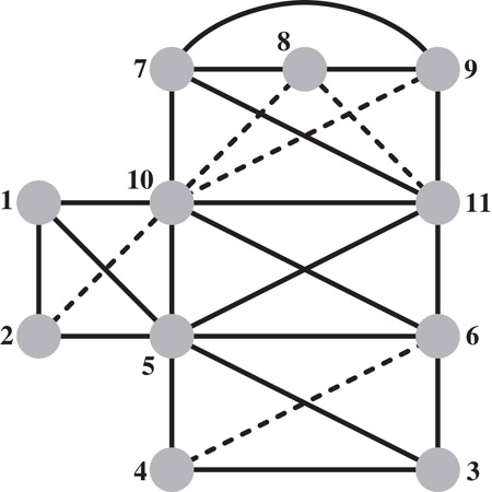
Figure 61.1A filled graph G+(A) resulting from the elimination game on a graph G(A). The solid edges belong to G(A), and the broken edges are filled edges generated by the elimination game when vertices are eliminated in the order shown.
The goal of the elimination game is to number the vertices to minimize the fill since it would reduce the storage needed to perform the factorization, and also controls the work in the factorization. Unfortunately, this is an NP-hard problem [5]. However, for classes of graphs that have small separators, it is possible to establish upper bounds on the number of edges in the filled graph, when the graph is ordered by a nested dissection algorithm that recursively computes separators. Planar graphs, graphs of “well-shaped” finite element meshes (aspect ratios bounded away from small values), and overlap graphs possess elimination orderings with bounded fill. Conversely, the fill is large for graphs that do not have good separators.
Approximation algorithms that incur fill within a polylog factor of the optimum fill have been designed by Agrawal, Klein and Ravi [6]; but since it involves finding approximate concurrent flows with uniform capacities, it is an impractical approach for large problems. A more recent approximation algorithm, due to Natanzon, Shamir and Sharan [7], limits fill to within the square of the optimal value; this approximation ratio is better than that of the former algorithm only for dense graphs.
The elimination game produces sets of cliques in the graph. Let hadj+(v) (ladj+(v)) denote the higher-numbered (lower-numbered) neighbors of a vertex v in the graph G+(A); in the elimination game, hadj+(v) is the set of unnumbered neighbors of v immediately prior to the step in which v is numbered. When a vertex v is numbered, the set {v} ∪ hadj+(v) becomes a clique by the rules of the elimination game. Future numbering steps and consequent fill edges added do not change the adjacency set (in the filled graph) of the vertex v. (We will use hadj(v) and ladj(v) to refer to higher and lower adjacency sets of a vertex v in the original graph G(A).)
61.1.2The Elimination Tree Data Structure
We define a forest from the filled graph by defining the parent of a vertex v to be the lowest numbered vertex in hadj+(v). It is clear that this definition of parent yields a forest since the parent of each vertex is numbered higher than itself. If the initial graph G(A) is connected, then indeed we have a tree, the elimination tree; if not we have an elimination forest.
In terms of the Cholesky factor L, the elimination tree is obtained by looking down each column below the diagonal element, and choosing the row index of the first subdiagonal nonzero to be the parent of a column. It will turn out that we can compute the elimination tree corresponding to a matrix and a given ordering without first computing the filled graph or the Cholesky factor.
The elimination tree of the graph in Figure 61.1 with the elimination ordering given there is shown in Figure 61.2.
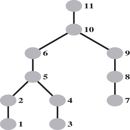
Figure 61.2The elimination tree of the example graph.
A fill path joining vertices i and j is a path in the original graph G(A) between vertices i and j, all of whose interior vertices are numbered lower than both i and j. The following theorem offers a static characterization of what causes fill in the elimination game.
Theorem 61.1: ([8])
The edge (i, j) is an edge in the filled graph if and only if a fill path joins the vertices i and j in the original graph G(A).
In the example graph in Figure 61.1, vertices 9 and 10 are joined a fill path consisting of the interior vertices 7 and 8; thus (9, 10) is a fill edge. The next theorem shows that an edge in the filled graph represents a dependence relation between its end points.
Theorem 61.2: ([9])
If (i, j) is an edge in the filled graph and i < j, then j is an ancestor of the vertex i in the elimination tree T(A).
This theorem suggests that the elimination tree represents the information flow in the elimination game (and hence sparse symmetric Gaussian elimination). Each vertex i influences only its higher numbered neighbors (the numerical values in the column i affect only those columns in hadj+(i)). The elimination tree represents the information flow in a minimal way in that we need consider only how the information flows from i to its parent in the elimination tree. If j is the parent of i and ℓ is another higher neighbor of i, then since the higher neighbors of i form a clique, we have an edge (j, ℓ) that joins j and ℓ; since by Theorem 61.2, ℓ is an ancestor of j, the information from i that affects ℓ can be viewed as being passed from i first to j, and then indirectly from j through its ancestors on the path in the elimination tree to ℓ.
An immediate consequence of the Theorem 61.2 is the following result.
Corollary 61.1
If vertices i and j belong to vertex-disjoint subtrees of the elimination tree, then no edge can join i and j in the filled graph.
Viewing the dependence relationships in sparse Cholesky factorization by means of the elimination tree, we see that any topological reordering of the elimination tree would be an elimination ordering with the same fill, since it would not violate the dependence relationships. Such reorderings would not change the fill or arithmetic operations needed in the factorization, but would change the schedule of operations in the factorization (i.e., when a specific operation is performed). This observation has been used in sparse matrix factorizations to schedule the computations for optimal performance on various computational platforms: multiprocessors, hierarchical memory machines, external memory algorithms, etc. A postordering of the elimination tree is typically used to improve the spatial and temporal data locality, and thereby the cache performance of sparse matrix factorizations.
There are two other perspectives from which we can view the elimination tree.
Consider directing each edge of the filled graph from its lower numbered endpoint to its higher numbered endpoint to obtain a directed acyclic graph (DAG). Now form the transitive reduction of the directed filled graph; that is, delete an edge (i, k) whenever there is a directed path from i to k that does not use the edge (i, k) (this path necessarily consists of at least two edges since we do not admit multiple edges in the elimination game). The minimal graph that remains when all such edges have been deleted is unique, and is the elimination tree.
One could also obtain the elimination tree by performing a depth-first search (DFS) in the filled graph with the vertex numbered n as the initial vertex for the DFS, and choosing the highest numbered vertex in ladj+(i) as the next vertex to search from a vertex i.
We begin with a consequence of the repeated application of the following fact: If a vertex i is adjacent to a higher numbered neighbor k in the filled graph, and k is not the parent of i, pi, in the elimination tree, then i is adjacent to both k and pi in the filled graph; when i is eliminated, by the rules of the elimination game, a fill edge joins pi and k.
Theorem 61.3
If (i, k) is an edge in the filled graph and i < k, then for every vertex j on an elimination tree path from i to k, (j, k) is also an edge in the filled graph.
This theorem leads to a characterization of ladj+(k), the set of lower numbered neighbors of a vertex k in the filled graph, which will be useful in designing an efficient algorithm for computing the elimination tree. The set ladj+(k) corresponds to the column indices of nonzeros in the kth row of the Cholesky factor L, and ladj(k) corresponds to the column indices of nonzeros in the lower triangle of the kth row of the initial matrix A.
Theorem 61.4: ([10])
Every vertex in the set ladj+(k) is a vertex reachable by paths in the elimination tree from a set of leaves to k; each leaf l corresponds to a vertex in the set ladj(k) such that no proper descendant d of l in the elimination tree belongs to the set ladj(k).
Theorem 61.4 characterizes the kth row of the Cholesky factor L as a row subtree Tr(k) of the elimination subtree rooted at the vertex k, and pruned at each leaf l. The leaves of the pruned subtree are contained among ladj(k), the column indices of the nonzeros in (the lower triangle of) the kth row of A. In the elimination tree in Figure 61.2, the pruned elimination subtree corresponding to row 11 has two leaves, vertices 5 and 7; it includes all vertices on the etree path from these leaves to the vertex 11.
The observation above leads to an algorithm, shown in Figure 61.3, for computing the elimination tree from the row structures of A, due to Liu [10].
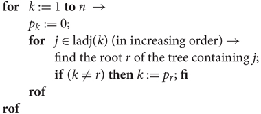
Figure 61.3An algorithm for computing an elimination tree. Initially each vertex is in a subtree with it as the root.
This algorithm can be implemented efficiently using the union-find data structure for disjoint sets. A height compressed version of the p. array, ancestor, makes it possible to compute the root fast; and union by rank in merging subtrees helps to keep the merged tree shallow. The time complexity of the algorithm is O(eα(e, n) + n), where n is the number of vertices and e is the number of edges in G(A), and α(e, n) is a functional inverse of Ackermann’s function. Liu [11] shows experimentally that path compression alone is more efficient than path compression and union by rank, although the asymptotic complexity of the former is higher. Zmijewski and Gilbert [12] have designed a parallel algorithm for computing the elimination tree on distributed memory multiprocessors.
The concept of the elimination tree was implicit in many papers before it was formally identified. The term elimination tree was first used by Duff [13], although he studied a slightly different data structure; Schreiber [9] first formally defined the elimination tree, and its properties were established and used in several articles by Liu. Liu [11] also wrote an influential survey that delineated its importance in sparse matrix computations; we refer the reader to this survey for a more detailed discussion of the elimination tree current as of 1990.
The filled graph represents a supergraph of the initial graph G(A), and a skeleton graph represents a subgraph of the latter. Many sparse matrix algorithms can be made more efficient by implicitly identifying the edges of a skeleton graph G−(A) from the graph G(A) and an elimination ordering, and performing computations only on these edges. A skeleton graph includes only the edges that correspond to the leaves in each row subtree in Theorem 61.4. The other edges in the initial graph G(A) can be discarded, since they will be generated as fill edges during the elimination game. Since each leaf of a row subtree corresponds to an edge in G(A), the skeleton graph G−(A) is indeed a subgraph of the former. The skeleton graph of the example graph is shown in Figure 61.4.
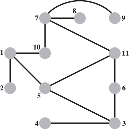
Figure 61.4The skeleton graph G−(A) of the example graph.
The leaves in a row subtree can be identified from the set ladj(j) when the elimination tree is numbered in a postordering. The subtree T(i) is the subtree of the elimination tree rooted at a vertex i, and |T(i)| is the number of vertices in that subtree. (It should not be confused with the row subtree Tr(i), which is a pruned subtree of the elimination tree.)
Theorem 61.5: ([10])
Let ladj(j) = {i1 < i2 < … < is}, and let the vertices of a filled graph be numbered in a postordering of its elimination tree T. Then vertex iq is a leaf of the row subtree Tr(j) if and only if either q = 1, or for q ≥ 2, .
A supernode is a subset of vertices S of the filled graph that form a clique and have the same higher neighbors outside S. Supernodes play an important role in numerical algorithms since loops corresponding to columns in a supernode can be blocked to obtain high performance on modern computer architectures. We now proceed to define a supernode formally.
A maximal clique in a graph is a set of vertices that induces a complete subgraph, but adding any other vertex to the set does not induce a complete subgraph. A supernode is a maximal clique in a filled graph G+(A) such that for each 1 ≤ j ≤ t − 1,
Let hd+(is) ≡ |hadj+(is)|; since , the relationship between the higher adjacency sets can be replaced by the equivalent test on higher degrees: hd+(is) = hd+(is+j) + j.
In practice, fundamental supernodes, rather than the maximal supernodes defined above, are used, since the former are easier to work with in the numerical factorization. A fundamental supernode is a clique but not necessarily a maximal clique, and satisfies two additional conditions: (1) is+j−1 is the only child of the vertex is+j in the elimination tree, for each 1 ≤ j ≤ t − 1; (2) the vertices in a supernode are ordered consecutively, usually by post-ordering the elimination tree. Thus vertices in a fundamental supernode form a path in the elimination tree; each of the non-terminal vertices in this path has only one child, and the child belongs to the supernode.
The fundamental supernodes corresponding to the example graph are: {1, 2}; {3, 4}; {5, 6}; {7, 8, 9}; and {10, 11}.
Just as we could compute the elimination tree directly from G(A) without first computing G+(A), we can compute fundamental supernodes without computing the latter graph, using the theorem given below. Once the elimination tree is computed, this algorithm can be implemented in O(n + e) time, where e ≡ |E| is the number of edges in the original graph G(A).
Theorem 61.6: ([14])
A vertex i is the first node of a fundamental supernode if and only if i has two or more children in the elimination tree T, or i is a leaf of some row subtree of T.
61.2.1Efficient Symbolic Factorization
Symbolic factorization (or symbolic elimination) is a process that computes the nonzero structure of the factors of a matrix without computing the numerical values of the nonzeros.
The symbolic Cholesky factor of a matrix has several uses. It is used to allocate the data structure for the numeric factor and annotate it with all the row/column indices, which enables the removal of most of the non-numeric operations from the inner-most loop of the subsequent numeric factorization [15,16]. It is also used to compute relaxed supernode (or amalgamated node) partitions, which group columns into supernodes even if they only have approximately the same structure [17,18]. Symbolic factors can also be used in algorithms that construct approximate Cholesky factors by dropping nonzeros from a matrix A and factoring the resulting, sparser matrix B [19,20]. In such algorithms, elements of A that are dropped from B but which appear in the symbolic factor of B can can be added to the matrix B; this improves the approximation without increasing the cost of factoring B. In all of these applications a supernodal symbolic factor (but not a relaxed one) is sufficient; there is no reason to explicitly represent columns that are known to be identical.
The following algorithm for symbolically factoring a symmetric matrix A is due to George and Liu [21] (and in a more graph-oriented form due to [8]; see also [16, Section 5.4.3] and [11, Section 8]).
The algorithm uses the elimination tree implicitly, but does not require it as input; the algorithm can actually compute the elimination tree on the fly. The algorithm uses the observation that
That is, the structure of a column of L is the union of the structure of its children in the elimination tree and the structure of the same column in the lower triangular part of A. Identifying the children can be done using a given elimination tree, or the elimination tree can be constructed on the fly by adding column i to the list of children of pi when the structure of i is computed (pi is the row index of the first subdiagonal nonzero in column i of L). The union of a set of column structures is computed using a boolean array P of size n (whose elements are all initialized to false), and an integer stack to hold the newly created structure. A row index k from a child column or from the column of A is added to the stack only if P[k] = false. When row index k is added to the stack, P[k] is set to true to signal that k is already in the stack. When the computation of hadj+(j) is completed, the stack is used to clear P so that it is ready for the next union operation. The total work in the algorithm is Θ(|L|), since each nonzero requires constant work to create and constant work to merge into the parent column, if there is a parent. (Here |L| denotes the number of nonzeros in L, or equivalently the number of edges in the filled graph G+(A); similarly |A| denotes the number of nonzeros in A, or the number of edges in the initial graph G(A).)
The symbolic structure of the factor can usually be represented more compactly and computed more quickly by exploiting supernodes, since we essentially only need to represent the identity of each supernode (the constituent columns) and the structure of the first (lowest numbered) column in each supernode. The structure of any column can be computed from this information in time proportional to the size of the column. The George-Liu column-merge algorithm presented above can compute a supernodal symbolic factorization if it is given as input a supernodal elimination tree; such a tree can be computed in O(|A|) time by the Liu-Ng-Peyton algorithm [14]. In practice, this approach saves a significant amount of work and storage.
Clearly, column-oriented symbolic factorization algorithms can also generate the structure of rows in the same asymptotic work and storage. But a direct symbolic factorization by rows is less obvious. Whitten [22], in an unpublished manuscript cited by Tarjan and Yannakakis [23], proposed a row-oriented symbolic factorization algorithm (see also [10] and [11, Sections 3.2 and 8.2]). The algorithm uses the characterization of the structure of row i in L as the row subtree Tr(i). Given the elimination tree and the structure of A by rows, it is trivial to traverse the ith row subtree in time proportional to the number of nonzeros in row i of L. Hence, the elimination tree along with a row-oriented representation of A is an effective implicit symbolic row-oriented representation of L; an explicit representation is usually not needed, but it can be generated in work and space O(|L|) from this implicit representation.
61.2.2Predicting Row and Column Nonzero Counts
In some applications the explicit structure of columns of L is not required, only the number of nonzeros in each column or each row. Gilbert, Ng, and Peyton [24] describe an almost-linear-time algorithm for determining the number of nonzeros in each row and column of L. Applications for computing these counts fast include comparisons of fill in alternative matrix orderings, preallocation of storage for a symbolic factorization, finding relaxed supernode partitions quickly, determining the load balance in parallel factorizations, and determining synchronization events in parallel factorizations.
The algorithm to compute row counts is based on Whitten’s characterization [22]. We are trying to compute . The column indices j < i in row i of A define a subset of the vertices in the subtree of the elimination tree rooted at the vertex i, T[i]. The difficulty, of course, is counting the vertices in Tr(i) without enumerating them. The Gilbert-Ng-Peyton algorithm counts these vertices using three relatively simple mechanisms: (1) processing the column indices j < i in row i of A in postorder of the etree, (2) computing the distance of each vertex in the etree from the root, and (3) setting up a data structure to compute the least-common ancestor (LCA) of pairs of etree vertices. It is not hard to show that the once these preprocessing steps are completed, |Tr(i)| can be computed using |Ai*| LCA computations. The total cost of the preprocessing and the LCA computations is almost linear in |A|.
Gilbert, Ng, and Peyton show how to further reduce the number of LCA computations. They exploit the fact that the leaves of Tr(i) are exactly the indices j that cause the creation of new supernodes in the Liu-Ng-Peyton supernode-finding algorithm [14]. This observation limits the LCA computations to leaves of row subtrees, that is, edges in the skeleton graph G−(A). This significantly reduces the running time in practice.
Efficiently computing the column counts in L is more difficult. The Gilbert-Ng-Peyton algorithm assigns a weight w(j) to each etree vertex j, such that . Therefore, the column-count of a vertex is the sum of the column counts of its children, plus its own weight. Hence, wj must compensate for (1) the diagonal elements of the children, which are not included in the column count for j, (2) for rows that are nonzero in column j but not in its children, and (3) for duplicate counting stemming from rows that appear in more than one child. The main difficulty lies in accounting for duplicates, which is done using least-common-ancestor computations, as in the row-counts algorithm. This algorithm, too, benefits from handling only skeleton-graph edges.
Gilbert, Ng, and Peyton [24] also show in their paper how to optimize these algorithms, so that a single pass over the nonzero structure of A suffices to compute the row counts, the column counts, and the fundamental supernodes.
61.2.3Three Classes of Factorization Algorithms
There are three classes of algorithms used to implement sparse direct solvers: left-looking, right-looking, and multifrontal; all of them use the elimination tree to guide the computation of the factors. The major difference between the first two of these algorithms is in how they schedule the computations they perform; the multifrontal algorithm organizes computations differently from the other two, and we explain this after introducing some concepts.
The computations on the sparse matrix are decomposed into subtasks involving computations among dense submatrices (supernodes), and the precedence relations among them are captured by the supernodal elimination tree. The computation at each node of the elimination tree (subtask) involves the partial factorization of the dense submatrix associated with it.
The right-looking algorithm is an eager updating scheme: Updates generated by the submatrix of the current subtask are applied immediately to future subtasks that it is linked to by edges in the filled graph of the sparse matrix. The left-looking algorithm is a lazy updating scheme: Updates generated by previous subtasks linked to the current subtask by edges in the filled adjacency graph of the sparse matrix are applied just prior to the factorization of the current submatrix. In both cases, updates always join a subtask to some ancestor subtask in the elimination tree. In the multifrontal scheme, updates always go from a child task to its parent in the elimination tree; an update that needs to be applied to some ancestor subtask is passed incrementally through a succession of vertices on the elimination tree path from the subtask to the ancestor.
Thus the major difference among these three algorithms is how the data accesses and the computations are organized and scheduled, while satisfying the precedence relations captured by the elimination tree. An illustration of these is shown in Figure 61.5.
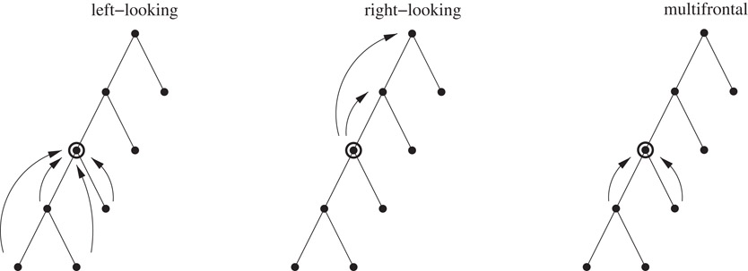
Figure 61.5Patterns of data access in the left-looking, right-looking, and multifrontal algorithms. A subtree of the elimination tree is shown, and the circled node corresponds to the current submatrix being factored.
61.2.4Scheduling Parallel Factorizations
In a parallel factorization algorithm, dependences between nonzeros in L determine the set of admissible schedules. A diagonal nonzero can only be factored after all updates to it from previous columns have been applied, a subdiagonal nonzero can be scaled only after updates to it have been applied (and after the diagonal element has been factored), and two subdiagonal nonzeros can update elements in the reduced system only after they have been scaled.
The elimination tree represents very compactly and conveniently a superset of these dependences. More specifically, the etree represents dependences between columns of L. A column can be completely factored only after all its descendants have been factored, and two columns that are not in an ancestor-descendant relationship can be factored in any order. Note that this is a superset of the element dependences, since a partially factored column can already perform some of the updates to its ancestors. But most sparse elimination algorithms treat column operations (or row operations) as atomic operations that are always performed by a single processor sequentially and with no interruption. For such algorithms, the etree represents exactly the relevant dependences.
In essence, parallel column-oriented factorizations can factor the columns associated with different children of an etree vertex simultaneously, but columns in an ancestor-descendant relationship must be processed in postorder. Different algorithms differ mainly in how updates are represented and scheduled.
By computing the number of nonzeros in each column, a parallel factorization algorithm can determine the amount of computation and storage associated with each subtree in the elimination tree. This information can be used to assign tasks to processors in a load-balanced way.
Duff was the first to observe that the column dependences represented by the elimination tree can guide a parallel factorization [25]. In that paper Duff proposed a parallel multifrontal factorization. The paper also proposed a way to deal with indefinite and asymmetric systems, similar to Duff and Reid’s sequential multifrontal approach [18]. For further references up to about 1997, see Heath’s survey [26]. Several implementations described in papers published after 1997 include PaStiX [27], PARADISO [28], WSSMP [29], and MUMPS [30], which also includes indefinite and unsymmetric factorizations. All four are message-passing codes.
61.2.5Scheduling Out-of-Core Factorizations
In an out-of-core factorization at least some of the data structures are stored on external-memory devices (today almost exclusively magnetic disks). This allows such factorization algorithms to factor matrices that are too large to factor in main memory. The factor, which is usually the largest data structure in the factorization, is the most obvious candidate for storing on disks, but other data structures, for example, the stack of update matrices in a multifrontal factorization, may also be stored on disks.
Planning and optimizing out-of-core factorization schedules require information about data dependences in the factorization and about the number of nonzeros in each column of the factor. The etree describes the required dependence information, and as explained above, it is also used to compute nonzero counts.
Following Rothberg and Schreiber [31], we classify out-of-core algorithms into robust algorithms and non-robust algorithms. Robust algorithms adapt the factorization to complete with the core memory available by performing the data movement and computations at a smaller granularity when necessary. They partition the submatrices corresponding to the supernodes and stacks used in the factorization into smaller units called panels to ensure that the factorization completes with the available memory. Non-robust algorithms assume that the stack or a submatrix corresponding to a supernode fits within the core memory provided. In general, non-robust algorithms read elements of the input matrix only once, read from disk nothing else, and they only write the factor elements to disk; Dobrian and Pothen refer to such algorithms as read-once-write-once, and to robust ones as read-many-write-many [32].
Liu proposed [33] a non-robust method that works as long as for all j = 1, …, n, all the nonzeros in the submatrix Lj:n,1:j of the factor fit simultaneously in main memory. Liu also shows in that paper how to reduce the amount of main memory required to factor a given matrix using this technique by reordering the children of vertices in the etree.
Rothberg and Schreiber [31,34] proposed a number of robust out-of-core factorization algorithms. They proposed multifrontal, left-looking, and hybrid multifrontal/left-looking methods. Rotkin and Toledo [35] proposed two additional robust methods, a more efficient left-looking method, and a hybrid right/left-looking method. All of these methods use the etree together with column-nonzero counts to organize the out-of-core factorization process.
Dobrian and Pothen [32] analyzed the amount of main memory required for read-once-write-once factorizations of matrices with several regular etree structures, and the amount of I/O that read-many-write-many factorizations perform on these matrices. They also provided simulations on problems with irregular elimination tree structures. These studies led them to conclude that an external memory sparse solver library needs to provide at least two of the factorization methods, since each method can out-perform the others on problems with different characteristics. They have provided implementations of out-of-core algorithms for all three of the multifrontal, left-looking, and right-looking factorization methods; these algorithms are included in the direct solver library OBLIO [36].
In addition to out-of-core techniques, there exist techniques that reduce the amount of main memory required to factor a matrix without using disks. Liu [37] showed how to minimize the size of the stack of update matrices in the multifrontal method by reordering the children of vertices in the etree; this method is closely related to [33]. Another approach, first proposed by Eisenstat, Schultz and Sherman [38] uses a block factorization of the coefficient matrix, but drops some of the off-diagonal blocks. Dropping these blocks reduces the amount of main memory required for storing the partial factor, but requires recomputation of these blocks when linear systems are solved using the partial factor. George and Liu [16, Chapter 6] proposed a general algorithm to partition matrices into blocks for this technique. Their algorithm uses quotient graphs, data structures that we describe later in this chapter.
61.3.1Chordal Graphs and Clique Trees
The filled graph G+(A) that results from the elimination game on the matrix A (the adjacency graph of the Cholesky factor L) is a chordal graph, that is, a graph in which every cycle on four or more vertices has an edge joining two non-consecutive vertices on the cycle [39]. (The latter edge is called a chord, whence the name chordal graph. This class of graphs has also been called triangulated or rigid circuit graphs.)
A vertex v in a graph G is simplicial if its neighbors adj(v) form a clique. Every chordal graph is either a clique, or it has two non-adjacent simplicial vertices. (The simplicial vertices in the filled graph in Figure 61.1 are 1, 2, 3, 4, 7, 8, and 9.) We can eliminate a simplicial vertex v without causing any fill by the rules of the elimination game, since adj(v) is already a clique, and no fill edge needs to be added. A chordal graph from which a simplicial vertex is eliminated continues to be a chordal graph. A perfect elimination ordering of a chordal graph is an ordering in which simplicial vertices are eliminated successively without causing any fill during the elimination game. A graph is chordal if and only if it has a perfect elimination ordering.
Suppose that the vertices of the adjacency graph G(A) of a sparse, symmetric matrix A have been re-numbered in an elimination ordering, and that G+(A) corresponds to the filled graph obtained by the elimination game on G(A) with that ordering. This elimination ordering is a perfect elimination ordering of the filled graph G+(A). Many other perfect elimination orderings are possible for G+(A), since there are at least two simplicial vertices that can be chosen for elimination at each step, until the graph has one uneliminated vertex.
It is possible to design efficient algorithms on chordal graphs whose time complexity is much less than O(|E ∪ F|), where E ∪ F denotes the set of edges in the chordal filled graph. This is accomplished by representing chordal graphs by tree data structures defined on the maximal cliques of the graph. (Recall that a clique K is maximal if K ∪ {v} is not a clique for any vertex v ∉ K.)
Theorem 61.7
Every maximal clique of a chordal filled graph G+(A) is of the form K(v) = {v} ∪ hadj+(v), with the vertices ordered in a perfect elimination ordering.
The vertex v is the lowest-numbered vertex in the maximal clique K(v), and is called the representative vertex of the clique. Since there can be at most n ≡ |V| representative vertices, a chordal graph can have at most n maximal cliques. The maximal cliques of the filled graph in Figure 61.1 are: K1 = {1, 2, 5, 10}; K2 = {3, 4, 5, 6}; K3 = {5, 6, 10, 11}; and K4 = {7, 8, 9, 10, 11}. The lowest-numbered vertex in each maximal clique is its representative; note that in our notation K2 = K(3), K1 = K(1), K3 = K(5), and K4 = K(7).
Let denote the set of maximal cliques of a chordal graph G. Define a clique intersection graph with the maximal cliques as its vertices, with two maximal cliques Ki and Kj joined by an edge (Ki, Kj) of weight |Ki ∩ Kj|. A clique tree corresponds to a maximum weight spanning tree (MST) of the clique intersection graph. Since the MST of a weighted graph need not be unique, a clique tree of a chordal graph is not necessarily unique either.
In practice, a rooted clique tree is used in sparse matrix computations. Lewis, Peyton, and Pothen [40] and Pothen and Sun [41] have designed algorithms for computing rooted clique trees. The former algorithm uses the adjacency lists of the filled graph as input, while the latter uses the elimination tree. Both algorithms identify representative vertices by a simple degree test. We will discuss the latter algorithm.
First, to define the concepts needed for the algorithm, consider that the the maximal cliques are ordered according to their representative vertices. This ordering partitions each maximal clique K(v) with representative vertex v into two subsets: new(K(v)) consists of vertices in the clique K(v) whose higher adjacency sets are contained in it but not in any earlier ordered maximal clique. The residual vertices in K(v)new(K(v)) form the ancestor set anc(K(v)). If a vertex w ∈ anc(K(v)), by definition of the ancestor set, w has a higher neighbor that is not adjacent to v; then by the rules of the elimination game, any higher-numbered vertex x ∈ K(v) also belongs to anc(K(v)). Thus the partition of a maximal clique into new and ancestor sets is an ordered partition: vertices in new(K(v)) are ordered before vertices in anc(K(v)). We denote the lowest numbered vertex f in anc(K(v)) the first ancestor of the clique K(v). A rooted clique tree may be defined as follows: the parent of a clique K(v) is the clique P in which the first ancestor vertex f of K appears as a vertex in new(P).
The reason for calling these subsets “new” and “ancestor” sets can be explained with respect to a rooted clique tree. We can build the chordal graph beginning with the root clique of the clique tree, successively adding one maximal clique at a time, proceeding down the clique tree in in-order. When a maximal clique K(v) is added, vertices in anc(K(v)) also belong to some ancestor clique(s) of K(v), while vertices in new(K(v)) appear for the first time. A rooted clique tree, with vertices in new(K) and anc(K) identified for each clique K, is shown in Figure 61.6.
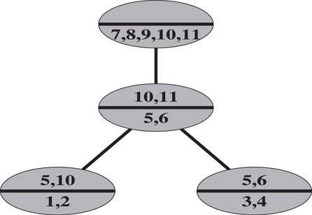
Figure 61.6A clique tree of the example filled graph, computed from its elimination tree. Within each clique K in the clique tree, the vertices in new(K) are listed below the bar, and the vertices in anc(K) are listed above the bar.
This clique tree algorithm can be implemented in O(n) time, once the elimination tree and the higher degrees have been computed. The rooted clique tree shown in Figure 61.6, is computed from the example elimination tree and higher degrees of the vertices in the example filled graph, using the clique tree algorithm described in Figure 61.7. The clique tree obtained from this algorithm is not unique. A second clique tree that could be obtained has the clique K(5) as the root clique, and the other cliques as leaves.
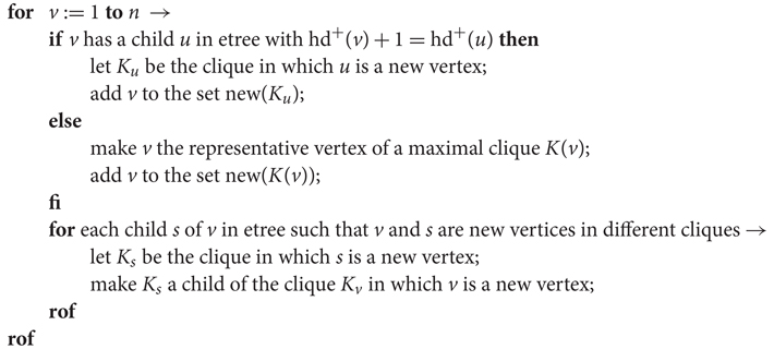
Figure 61.7An algorithm for computing a clique tree from an elimination tree, whose vertices are numbered in postorder. The variable hd+(v) is the higher degree of a vertex v in the filled graph.
A comprehensive review of clique trees and chordal graphs in sparse matrix computations, current as of 1991, is provided by Blair and Peyton [42].
61.3.2Design of Efficient Algorithms with Clique Trees
Shortest Elimination Trees. Jess and Kees [43] introduced the problem of modifying a fill-reducing elimination ordering to enhance concurrency in a parallel factorization algorithm. Their approach was to generate a chordal filled graph from the elimination ordering, and then to eliminate a maximum independent set of simplicial vertices at each step, until all the vertices are eliminated. (This is a greedy algorithm in which the largest number of pairwise independent columns that do not cause fill are eliminated in one step.) Liu and Mirzaian [44] showed that this approach computed a shortest elimination tree over all perfect elimination orderings for a chordal graph, and provided an implementation linear in the number of edges of the filled graph. Lewis, Peyton, and Pothen [44] used the clique tree to provide a faster algorithm; their algorithm runs in time proportional to the size of the clique tree: the sum of the sizes of the maximal cliques of the chordal graph.
A vertex is simplicial if and only if it belongs to exactly one maximal clique in the chordal graph; a maximum independent set of simplicial vertices is obtained by choosing one such vertex from each maximal clique that contains simplicial vertices, and thus the clique tree is a natural data structure for this problem. The challenging aspect of the algorithm is to update the rooted clique tree when simplicial vertices are eliminated and cliques that become non-maximal are absorbed by other maximal cliques.
Parallel Triangular Solution. In solving systems of linear equations by factorization methods, usually the work involved in the factorization step dominates the work involved in the triangular solution step (although the communication costs and synchronization overheads of both steps are comparable). However, in some situations, many linear systems with the same coefficient matrix but with different right-hand-side vectors need to be solved. In such situations, it is tempting to replace the triangular solution step involving the factor matrix L by explicitly computing an inverse L−1 of the factor. Unfortunately L−1 can be much less sparse than the factor, and so a more space efficient “product-form inverse” needs to be employed. In this latter form, the inverse is represented as a product of triangular matrices such that all the matrices in the product together require exactly as much space as the original factor.
The computation of the product form inverse leads to some interesting chordal graph partitioning problems that can be solved efficiently by using a clique tree data structure.
We begin by directing each edge in the chordal filled graph G+(A) from its lower to its higher numbered end point to obtain a directed acyclic graph (DAG). We will denote this DAG by G(L). Given an edge (i, j) directed from i to j, we will call i the predecessor of j, and j the successor of i. The elimination ordering must eliminate vertices in a topological ordering of the DAG such that all predecessors of a vertex must be eliminated before it can be eliminated. The requirement that each matrix in the product form of the inverse must have the same nonzero structure as the corresponding columns in the factor is expressed by the fact that the subgraph corresponding to the matrix should be transitively closed. (A directed graph is transitively closed if whenever there is a directed path from a vertex i to a vertex j, there is an edge directed from i to j in the graph.) Given a set of vertices Pi, the column subgraph of Pi includes all the vertices in Pi and vertices reached by directed edges leaving vertices in Pi; the edges in this subgraph include all edges with one or both endpoints in Pi.
The simpler of the graph partitioning problems is the following:
Find an ordered partition P1 ≺ P2 ≺ … Pm of the vertices of a directed acyclic filled graph G(L) such that
1.Every v ∈ Pi has all of its predecessors included in P1, …, Pi;
2.The column subgraph of Pi is transitively closed; and
3.The number of subgraphs m is minimum over all topological orderings of G(L).
Pothen and Alvarado [45] designed a greedy algorithm that runs in O(n) time to solve this partitioning problem by using the elimination tree.
A more challenging variant of the problem minimizes the number of transitively closed subgraphs in G(L) over all perfect elimination orderings of the undirected chordal filled graph G+(A). This variant could change the edges in the DAG G(L), (but not the edges in G+(A)) since the initial ordering of the vertices is changed by the perfect elimination ordering, and after the reordering, edges are directed from the lower numbered end point to its higher numbered end point.
This is quite a difficult problem, but two surprisingly simple greedy algorithms solve it. Peyton, Pothen, and Yuan provide two different algorithms for this problem; the first algorithm uses the elimination tree and runs in time linear in the number of edges in the filled graph [46]. The second makes use of the clique tree, and computes the partition in time linear in the size of the clique tree [47]. Proving the correctness of these algorithms requires a careful study of the properties of the minimal vertex separators (these are vertices in the intersections of the maximal cliques) in the chordal filled graph.
In analogy with skeleton graphs, we can define a space-efficient version of a clique tree representation of a chordal graph, called the compact clique tree. If K is the parent clique of a clique C in a clique tree, then it can be shown that anc(C) ⊂ K. Thus trading space for computation, we can delete the vertices in K that belong to the ancestor sets of its children, since we can recompute them when necessary by unioning the ancestor sets of the children. The partition into new and ancestor sets can be obtained by storing the lowest numbered ancestor vertex for each clique. A compact clique Kc corresponding to a clique K is:
Note that the compact clique depends on the specific clique tree from which it is computed.
A compact clique tree is obtained from a clique tree by replacing cliques by compact cliques for vertices. In the example clique tree, the compact cliques of the leaves are unchanged from the corresponding cliques; and the compact cliques of the interior cliques are Kc(5) = {11}, and Kc(7) = {7, 8, 9}.
The compact clique tree is potentially sparser (asymptotically O(n) instead of O(n2) even) than the skeleton graph on pathological examples, but on “practical” examples, the size difference between them is small. Compact clique trees were introduced by Pothen and Sun [41].
61.4Clique Covers and Quotient Graphs
Clique covers and quotient graphs are data structures that were developed for the efficient implementation of minimum-degree reordering heuristics for sparse matrices. In Gaussian elimination, an elimination step that uses aij as a pivot (the elimination of the jth unknown using the ith equation) modifies every coefficient akl for which akj ≠ 0 and ail ≠ 0. Minimum-degree heuristics attempt to select pivots for which the number of modified coefficients is small.
Recall the graph model of symmetric Gaussian elimination discussed in Section 61.1.1. The adjacency graph of the matrix to be factored is an undirected graph G = (V, E), V = {1, 2, …, n}, E = {(i, j):aij ≠ 0}. The elimination of a row/column j corresponds to eliminating vertex j and adding edges to the remaining graph so that the neighbors of j become a clique. If we represent the edge set E using a clique cover, a set of cliques such that , the vertex elimination process becomes a process of merging cliques [39]: The elimination of vertex j corresponds to merging all the cliques that j belongs to into one clique and removing j from all the cliques. Clearly, all the old cliques that j used to belong to are now covered by the new clique, so they can be removed from the cover. The clique-cover can be initialized by representing every nonzero of A by a clique of size 2. This process corresponds exactly to symbolic elimination, which we have discussed in Section 61.2, and which costs Θ(|L|) work. The cliques correspond exactly to frontal matrices in the multifrontal factorization method.
In the sparse-matrix literature, this model of Gaussian elimination has been sometimes called the generalized-element model or the super-element model, due to its relationship to finite-element models and matrices.
The significance of clique covers is due to the fact that in minimum-degree ordering codes, there is no need to store the structure of the partially computed factor, so when one clique is merged into another, it can indeed be removed from the cover. This implies that the total size of the representation of the clique cover, which starts at exactly |A| − n, shrinks in every elimination step, so it is always bounded by |A| − n. Since exactly one clique is formed in every elimination step, the total number of cliques is also bounded, by n + (|A| − n) = |A|. In contrast, the storage required to explicitly represent the symbolic factor, or even to just explicitly represent the edges in the reduced matrix, can grow in every elimination step and is not bounded by O(|A|).
Some minimum-degree codes represent cliques fully explicitly [48,49]. This representation uses an array of cliques and an array of vertices; each clique is represented by a linked list of vertex indices, and each vertex is represented by a linked list of clique indices to which it belongs. The size of this data structure never grows—linked-list elements are moved from one list to another or are deleted during elimination steps, but new elements never need to be allocated once the data structure is initialized.
Most codes, however, use a different representation for clique covers, which we describe next.
Most minimum-degree codes represent the graphs of reduced matrices during the elimination process using quotient graphs [50]. Given a graph G = (V, E) and a partition of V into disjoint sets , the quotient graph is the undirected graph where .
The representation of a graph G after the elimination of vertices 1, 2, …, j − 1, but before the elimination of vertex j, uses a quotient graph , where consists of sets Sk of eliminated vertices that form maximal connected components in G, and sets Si = {i} of uneliminated vertices i ≥ j. We denote a set Sk of eliminated vertices by the index k of the highest-numbered vertex in it.
This quotient graph representation of an elimination graph corresponds to a clique cover representation as follows. Each edge in the quotient graph between uneliminated vertices and corresponds to a clique of size 2; all the neighbors of an eliminated set Sk correspond to a clique, the clique that was created when vertex k was eliminated. Note that all the neighbors of an uneliminated set Sk are uneliminated vertices, since uneliminated sets are maximal with respect to connectivity in G.
The elimination of vertex j in the quotient-graph representation corresponds to marking Sj as eliminated and merging it with its eliminated neighbors, to maintain the maximal connectivity invariant.
Clearly, a representation of the initial graph G using adjacency lists is also a representation of the corresponding quotient graph. George and Liu [51] show how to maintain the quotient graph efficiently using this representation without allocating more storage through a series of elimination steps.
Most of the codes that implement minimum-degree ordering heuristics, such as GENMMD [52], AMD [53], and Spindle [54,55], use quotient graphs to represent elimination graphs.
It appears that the only advantage of a quotient graph over an explicit clique cover in the context of minimum-degree algorithms is a reduction by a small constant factor in the storage requirement, and possibly in the amount of work required. Quotient graphs, however, can also represent symmetric partitions of symmetric matrices in applications that are not directly related to elimination graphs. For example, George and Liu use quotient graphs to represent partitions of symmetric matrices into block matrices that can be factored without fill in blocks that only contain zeros [16, Chapter 6].
In [56], George and Liu showed how to implement the minimum degree algorithm without modifying the representation of the input graph at all. In essence, this approach represents the quotient graph implicitly using the input graph and the indices of the eliminated vertices. The obvious drawback of this approach is that vertex elimination (as well as other required operations) are expensive.
61.4.3The Problem of Degree Updates
The minimum-degree algorithm works by repeatedly eliminating the vertex with the minimum degree and turning its neighbors into a clique. If the reduced graph is represented by a clique cover or a quotient graph, then the representation does not reveal the degree of vertices. Therefore, when a vertex is eliminated from a graph represented by a clique cover or a quotient graph, the degrees of its neighbors must be recomputed. These degree updates can consume much of the running time of minimum-degree algorithms.
Practical minimum-degree codes use several techniques to address this issue. Some techniques reduce the running time while preserving the invariant that the vertex that is eliminated always has the minimum degree. For example, mass elimination, the elimination of all the vertices of a supernode consecutively without recomputing degrees, can reduce the running time significantly without violating this invariant. Other techniques, such as multiple elimination and the use of approximate degrees, do not preserve the minimum-degree invariant. This does not imply that the elimination orderings that such technique produce are inferior to true minimum-degree orderings. They are often superior to them. This is not a contradiction since the minimum-degree rule is just a heuristic which is rarely optimal. For further details, we refer the reader to George and Liu’s survey [57], to Amestoy, Davis, and Duff’s paper on approximate minimum-degree rules [53], and to Kumfert and Pothen’s work on minimum-degree variants [54,55]. Heggernes, Eisenstat, Kumfert and Pothen prove upper bounds on the running time of space-efficient minimum-degree variants [58].
61.4.4Covering the Column-Intersection Graph and Biclique Covers
Column orderings for minimizing fill in Gaussian elimination with partial pivoting and in the orthogonal-triangular (QR, where Q is an orthogonal matrix, and R is an upper triangular matrix) factorization are often based on symmetric fill minimization in the symmetric factor of ATA, whose graph is known as the the column intersection graph G∩(A) (we ignore the possibility of numerical cancellation in ATA). To run a minimum-degree algorithm on the column intersection graph, a clique cover or quotient graph of it must be constructed. One obvious solution is to explicitly compute the edge-set of G∩(A), but this is inefficient, since G∩(A) can be much denser than G(A).
A better solution is to initialize the clique cover using a clique for every row of A; the vertices of the clique are the indices of the nonzeros in that row [57]. It is easy to see that each row in A indeed corresponds to a clique in G∩(A). This approach is used in the COLMMD routine in MATLAB [49] and in COLAMD [59].
A space-efficient quotient-graph representation for G∩(A) can be constructed by creating an adjacency-list representation of the symmetric 2-by-2 block matrix
and eliminating vertices 1 through n. The graph of the Schur complement matrix
If we maintain a quotient-graph representation of the reduced graph through the first n elimination steps, we obtain a space-efficient quotient graph representation of the column-intersection graph. This is likely to be more expensive, however, than constructing the clique-cover representation from the rows of A. We learned of this idea from John Gilbert; we are not aware of any practical code that uses it.
The nonzero structure of the Cholesky factor of ATA is only an upper bound on the structure of the LU factors in Gaussian elimination with partial pivoting. If the identities of the pivots are known, the nonzero structure of the reduced matrices can be represented using biclique covers. The nonzero structure of A is represented by a bipartite graph ({1, 2, …, n} ∪ {1′, 2′, …, n′}, {(i, j′): aij ≠ 0}). A biclique is a complete bipartite graph on a subset of the vertices. Each elimination step corresponds to a removal of two connected vertices from the bipartite graph, and an addition of a new biclique. The vertices of the new biclique are the neighbors of the two eliminated vertices, but they are not the union of a set of bicliques. Hence, the storage requirement of this representation may exceed the storage required for the initial representation. Still, the storage requirement is always smaller than the storage required to represent each edge of the reduced matrix explicitly. This representation poses the same degree update problem that symmetric clique covers pose, and the same techniques can be used to address it. Version 4 of UMFPACK, an asymmetric multifrontal LU factorization code, uses this idea together with a degree approximation technique to select pivots corresponding to relatively sparse rows in the reduced matrix [60].
61.5Column Elimination Trees and Elimination DAGS
Elimination structures for asymmetric Gaussian elimination are somewhat more complex than the equivalent structures for symmetric elimination. The additional complexity arises because of two issues. First, the factorization of a sparse asymmetric matrix A, where A is factored into a lower triangular factor L and an upper triangular factor U, A = LU, is less structured than the sparse symmetric factorization process. In particular, the relationship between the nonzero structure of A and the nonzero structure of the factors is much more complex. Consequently, data structures for predicting fill and representing data-flow and control-flow dependences in elimination algorithms are more complex and more diverse.
Second, factoring an asymmetric matrix often requires pivoting, row and/or column exchanges, to ensure existence of the factors and numerical stability. For example, the 2-by-2 matrix A = [0 1; 1 0] does not have an LU factorization, because there is no way to eliminate the first variable from the first equation: that variable does not appear in the equation at all. But the permuted matrix PA does have a factorization, if P is a permutation matrix that exchanges the two rows of A. In finite precision arithmetic, row and/or column exchanges are necessary even when a nonzero but small diagonal element is encountered. Some sparse LU algorithms perform either row or column exchanges, but not both. The two cases are essentially equivalent (we can view one as a factorization of AT), so we focus on row exchanges (partial pivoting). Other algorithms, primarily multifrontal algorithms, perform both row and column exchanges; these are discussed toward the end of this section.
For completeness, we note that pivoting is also required in the factorization of sparse symmetric indefinite matrices. Such matrices are usually factored into a product LDLT, where L is lower triangular and D is a block diagonal matrix with 1-by-1 and 2-by-2 blocks. There has not been much research about specialized elimination structures for these factorization algorithms; such codes invariably use the symmetric elimination tree of A to represent dependences for structure prediction and for scheduling the factorization.
The complexity and diversity of asymmetric elimination arises not only due to pivoting, but also because asymmetric factorizations are less structured than symmetric ones, so a rooted tree can no longer represent the factors. Instead, directed acyclic graphs (dags) are used to represent the factors and dependences in the elimination process. We discuss elimination dags (edags) in Section 61.5.2.
Surprisingly, dealing with partial pivoting turns out to be simpler than dealing with the asymmetry, so we focus next on the column elimination tree, an elimination structure for LU factorization with partial pivoting.
61.5.1The Column Elimination Tree
The column elimination tree (col-etree) is the elimination tree of ATA, under the assumption that no numerical cancellation occurs in the formation of ATA. The significance of this tree to LU with partial pivoting stems from a series of results that relate the structure of the LU factors of PA, where P is some permutation matrix, to the structure of the Cholesky factor of ATA.
George and Ng observed that, for any permutation matrix P, the structure of the LU factors of PA is contained in the structure of the Cholesky factor of ATA, as long as A does not have any zeros on its main diagonal [61]. (If there are zeros on the diagonal of a nonsingular A, the rows can always be permuted first to achieve a zero-free diagonal.) Figure 61.8 illustrates this phenomenon. Gilbert [62] strengthened this result by showing that for every nonzero Rij in the Cholesky factor R of ATA = RTR, where A has a zero-free diagonal and no nontrivial block triangular form, there exists a matrix A(Uij) with the same nonzero structure as A, such that in the LU factorization of with partial pivoting, . This kind of result is known as a one-at-a-time result, since it guarantees that every element of the predicted factor can fill for some choice of numerical values in A, but not that all the elements can fill simultaneously. Gilbert and Ng [63] later generalized this result to show that an equivalent one-at-a-time property is true for the lower-triangular factor.
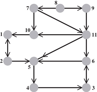
Figure 61.8The directed graph G(A) of an asymmetric matrix A. The column intersection graph of this graph G∩(B) is exactly the graph shown in Figure 61.1, so the column elimination tree of A is the elimination tree shown in Figure 61.2. Note that the graph is sparser than the column intersection graph.
These results suggest that the col-etree, which is the elimination tree of ATA, can be used for scheduling and structure prediction in LU factorizations with partial pivoting. Because the characterization of the nonzero structure of the LU factors in terms of the structure of the Cholesky factor of ATA relies on one-at-a-time results, the predicted structure and predicted dependences are necessarily only loose upper bounds, but they are nonetheless useful.
The col-etree is indeed useful in LU with partial pivoting. If Uij ≠ 0, then by the results cited above Rij ≠ 0 (recall that R is the Cholesky factor of the matrix ATA). This, in turn, implies that j is an ancestor of i in the col-etree. Since column i of L updates column j of L and U only if Uij ≠ 0, the col-etree can be used as a task-dependence graph in column-oriented LU factorization codes with partial pivoting. This analysis is due to Gilbert, who used it to schedule a parallel factorization code [62]. The same technique is used in several current factorization codes, including SuperLU [64], SuperLU_MT [65], UMFPACK 4 [60], and TAUCS [66,67]. Gilbert and Grigori [68] recently showed that this characterization is tight in a strong all-at-once sense: for every strong Hall matrix A (i.e., A has no nontrivial block-triangular form), there exists a permutation matrix P such that every edge of the col-etree corresponds to a nonzero in the upper-triangular factor of PA. This implies that the a-priori symbolic column-dependence structure predicted by the col-etree is as tight as possible.
Like the etree of a symmetric matrix, the col-etree can be computed in time almost linear in the number of nonzeros in A [69]. This is done by an adaptation of the symmetric etree algorithm, an adaptation that does not compute explicitly the structure of ATA. Instead of constructing G(ATA), the algorithm constructs a much sparser graph G′ with the same elimination tree. The main idea is that each row of A contributes a clique to G(ATA); this means that each nonzero index in the row must be an ancestor of the preceding nonzero index. A graph in which this row-clique is replaced by a path has the same elimination tree, and it has only as many edges as there are nonzeros in A. The same paper shows not only how to compute the col-etree in almost linear time, but also how to bound the number of nonzeros in each row and column of the factors L and U, using again an extension of the symmetric algorithm to compute the number of nonzeros in the Cholesky factor of ATA. The decomposition of this Cholesky factor into fundamental supernodes, which the algorithm also computes, can be used to bound the extent of fundamental supernodes that will arise in L.
The col-etree represents all possible column dependences for any sequence of pivot rows. For a specific sequence of pivots, the col-etree includes dependences that do not occur during the factorization with these pivots. There are two typical situations in which the pivoting sequence is known. The first is when the matrix is known to have a stable LU factorization without pivoting. The most common case is when AT is strictly diagonally dominant. Even if A is not diagonally dominant, its rows can be pre-permuted to bring large elements to the diagonal. The permuted matrix, even if its transpose is not diagonally dominant, is fairly likely to have a relatively stable LU factorization that can be used to accurately solve linear systems of equations. This strategy is known as static pivoting [70]. The other situation in which the pivoting sequence is known is when the matrix, or part of it, has already been factored. Since virtually all sparse factorization algorithms need to collect information from the already-factored portion of the matrix before they factor the next row and column, a compact representation of the structure of this portion is useful.
Elimination dags (edags) are directed acyclic graphs that capture a minimal or near minimal set of dependences in the factors. Several edags have been proposed in the literature. There are two reasons for this diversity. First, edags are not always as sparse and easy to compute as elimination trees, so researchers have tried to find edags that are easy to compute, even if they represent a superset of the actual dependences. Second, edags often contain information only about a specific structure in the factors or a specific dependence in a specific elimination algorithm (e.g., data dependence in a multifrontal algorithm), so different edags are used for different applications. In other words, edags are not as universal as etrees in their applications.
The simplest edag is the graph G(LT) of the transpose of the lower triangular factor, if we view every edge in this graph as directed from the lower-numbered vertex to a higher-numbered vertex. This corresponds to orienting edges from a row index to a column index in L. For example, if L6,3 ≠ 0, we view the edge (6, 3) as a directed edge in G(LT). Let us denote by the partial lower triangular factor after j − 1 columns have been factored. Gilbert and Peierls showed that the nonzeros in the jth rows of L and U are exactly the vertices reachable, in , from the nonzero indices in the jth column of A [71]. This observation allowed them to use a depth-first search (DFS) to quickly find the columns in the already-factored part of the matrix that update the jth column before it can be factored. This resulted in the first algorithm that factored a general sparse matrix in time linear in the number of arithmetic operations (earlier algorithms sometimes performed much more work to manipulate the sparse data structure than the amount of work in the actual numerical computations).
Eisenstat and Liu showed that a simple modification of the graph can often eliminate many of its edges without reducing its ability to predict fill [72]. They showed that if both Lik and Uki are nonzeros, then all the edges for ℓ > i can be safely pruned from the graph. In other words, the nonzeros in column k of L below row i can be pruned. This is true since if Uki ≠ 0, then column k of L updates column i, so all the pruned nonzeros appear in column i, and since the edge is in the graph, they are all reachable when k is reachable. This technique is called symmetric pruning. This edag is used in the SuperLU codes [64,65] to find the columns that update the next supernode (set of consecutive columns with the same nonzero structure in L). Note that the same codes use the col-etree to predict structure before the factorization begins, and an edag to compactly represent the structure of the already-factored block of A.
Gilbert and Liu went a step further and studied the minimal edags that preserve the reachability property that is required to predict fill [73]. These graphs, which they called the elimination dags are the transitive reductions of the directed graphs G(LT) and G(U). (The graph of U can be used to predict the row structures in the factors, just as G(LT) can predict the column structures.) Since these graphs are acyclic, each graph has a unique transitive reduction; If A is symmetric, the transitive reduction is the symmetric elimination tree. For the graph G(A) shown in Figure 61.8, the graph of the upper triangular factor G(U) is depicted in Figure 61.9, and its minimal edag is shown in Figure 61.10. Gilbert and Liu also proposed an algorithm to compute these transitive reductions row by row. Their algorithm computes the next row i of the transitive reduction of L by traversing the reduction of U to compute the structure of row i of L, and then reducing it. Then the algorithm computes the structure of row i of U by combining the structures of earlier rows whose indices are the nonzeros in row i of L. In general, these minimal edags are often more expensive to compute than the symmetrically-pruned edags, due to the cost of transitively reducing each row. Gupta recently proposed a different algorithm for computing the minimal edags [74]. His algorithm computes the minimal structure of U by rows and of L by columns. His algorithm essentially applies to both L and U the rule that Gilbert and Liu apply to U. By computing the structure of U by rows and of L by columns, Gupta’s algorithm can cheaply detect supernodes that are suitable for asymmetric multifrontal algorithms, where a supernode consists of a set of consecutive indices for which both the rows of U all have the same structure and the columns of L have the same structure (but the rows and columns may have different structures).
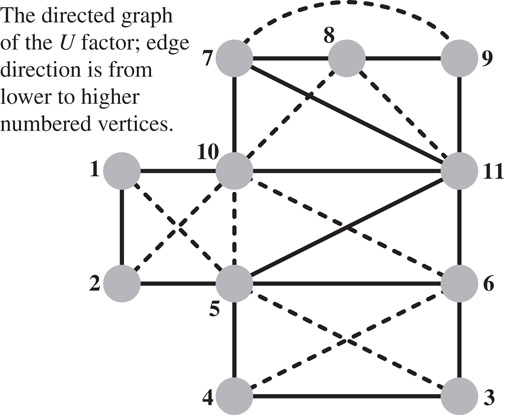
Figure 61.9The directed graph of the U factor of the matrix whose graph is shown in Figure 61.8. In this particular case, the graph of LT is exactly the same graph, only with the direction of the edges reversed. Fill is indicated by dashed lines. Note that the fill is indeed bounded by the fill in the column-intersection graph, which is shown in Figure 61.1. However, that upper bound is not realized in this case: the edge (9, 10) fills in the column-intersection graph, but not in the LU factors.
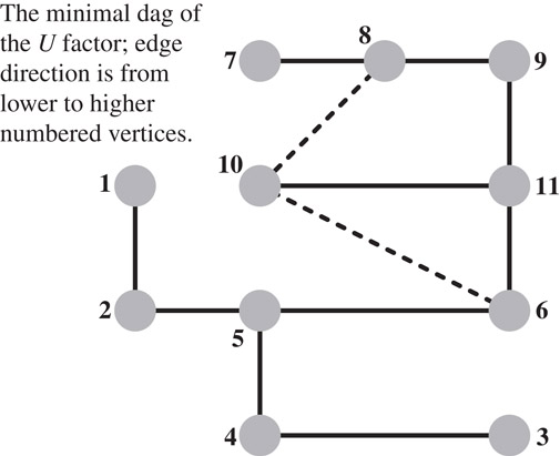
Figure 61.10The minimal edag of U; this graph is the transitive reduction of the graph shown in Figure Figure 61.9.
61.5.3Elimination Structures for the Asymmetric Multifrontal Algorithm
Asymmetric multifrontal LU factorization algorithms usually use both row and column exchanges. UMFPACK, the first such algorithm, due to Davis and Duff [75], used a pivoting strategy that factored an arbitrary row and column permutation of A. The algorithm tried to balance numerical and degree considerations in selecting the next row and column to be factored, but in principle, all row and column permutations were possible. Under such conditions, not much structure prediction is possible. The algorithm still used a clever elimination structure that we described earlier, a biclique cover, to represent the structure of the Schur complement (the remaining uneliminated equations and variables), but it did not use etrees or edags.
Recent unsymmetric multifrontal algorithms still use pivoting strategies that allow both row and column exchanges, but the pivoting strategies are restricted enough that structure prediction is possible. These pivoting strategies are based on delayed pivoting, which was originally invented for symmetric indefinite factorizations. One such code, Davis’s UMFPACK 4, uses the column elimination tree to represent control-flow dependences, and a biclique cover to represent data dependences [60]. Another code, Gupta’s WSMP, uses conventional minimal edags to represent control-flow dependences, and specialized dags to represent data dependences [74]. More specifically, Gupta shows how to modify the minimal edags so they exactly represent data dependences in the unsymmetric multifrontal algorithm with no pivoting, and how to modify the edags to represent dependences in an unsymmetric multifrontal algorithm that employs delayed pivoting.
Alex Pothen was supported, in part, by the National Science Foundation under grant CCR-0306334, and by the Department of Energy under subcontract DE-FC02-01ER25476. Sivan Toledo was supported in part by an IBM Faculty Partnership Award, by grant 572/00 from the Israel Science Foundation (founded by the Israel Academy of Sciences and Humanities), and by Grant 2002261 from the US-Israeli Binational Science Foundation.
1.A. George, J. R. Gilbert and J. W. H. Liu, editors Graph Theory and Sparse Matrix Computation. Springer-Verlag, New York, 1993. IMA Volumes in Applied Mathematics, Volume 56.
2.I. S. Duff. Sparse numerical linear algebra: direct methods and preconditioning. Technical Report RAL-TR-96-047, Department of Computation and Information, Rutherford Appleton Laboratory, Oxon OX11 0QX, England, 1996.
3.S. V. Parter. The use of linear graphs in Gaussian elimination. SIAM Review, 3:119–130, 1961.
4.R. E. Tarjan. Unpublished lecture notes. 1975.
5.M. Yannakakis. Computing the minimum fill-in is NP-complete. SIAM Journal on Algebraic and Discrete Methods, 2:77–79, 1981.
6.A. Agrawal, P. Klein, and R. Ravi. Cutting down on fill using nested dissection: Provably good elimination orderings. In [1], pages 31–55, 1993.
7.A. Natanzon, R. Shamir, and R. Sharan. A polynomial approximation algorithm for the minimum fill-in problem. In Proceedings of the 30th Annual ACM Symposium on the Theory of Computing (STOC 98), Dallas, TX, pages 41–47, 1998.
8.D. J. Rose, R. E. Tarjan, and G. S. Lueker. Algorithmic aspects of vertex elimination on graphs. SIAM Journal on Computing, 5:266–283, 1976.
9.R. S. Schreiber. A new implementation of sparse Gaussian elimination. ACM Transactions on Mathematical Software, 8:256–276, 1982.
10.J. W. H. Liu. A compact row storage scheme for Cholesky factors using elimination trees. ACM Transactions on Mathematical Software, 12(2):127–148, 1986.
11.J. W. H. Liu. The role of elimination trees in sparse factorization. SIAM Journal on Matrix Analysis and Applications, 11:134–172, 1990.
12.E. Zmijewski and J. R. Gilbert. A parallel algorithm for sparse symbolic Cholesky factorization on a multiprocessor. Parallel Computing, 7:199–210, 1988.
13.I. S. Duff. Full matrix techniques in sparse matrix factorizations. In G. A. Watson, editor, Lecture Notes in Mathematics, pages 71–84. Springer-Verlag, 1982.
14.J. W. H. Liu, E. G. Ng, and B. W. Peyton. On finding supernodes for sparse matrix computations. SIAM Journal on Matrix Analysis and Applications, 14:242–252, 1993.
15.I. S. Duff, A. M. Erisman, and J. K. Reid. Direct Methods for Sparse Matrices, Second edition. Oxford University Press, Oxford, 2017.
16.A. George and J. W. H. Liu. Computer Solution of Large Sparse Positive Definite Systems. Prentice-Hall, 1981.
17.C. Ashcraft and R. Grimes. The influence of relaxed supernode partitions on the multifrontal method. ACM Transactions on Mathematical Software, 15(4):291–309, 1989.
18.I. S. Duff and J. K. Reid. The multifrontal solution of indefinite sparse symmetric linear equations. ACM Transactions on Mathematical Software, 9:302–325, 1983.
19.M. Bern, J. R. Gilbert, B. Hendrickson, N. Nguyen, and S. Toledo. Support-graph preconditioners. SIAM Journal on Matrix Analysis and Applications, 27(4), 930–951, 2006.
20.P. M. Vaidya. Solving linear equations with symmetric diagonally dominant matrices by constructing good preconditioners. Unpublished manuscript. A talk based on the manuscript was presented at the IMA Workshop on Graph Theory and Sparse Matrix Computation, Minneapolis October 1991.
21.A. George and J. W. H. Liu. An optimal algorithm for symbolic factorization of symmetric matrices. SIAM Journal on Computing, 9:583–593, 1980.
22.G. F. Whitten. Computation of fill-in for sparse symmetric positive definite matrices. Technical report, Computer Science Department, Vanderbilt University, Nashville, TN, 1978.
23.R. E. Tarjan and M. Yannakakis. Simple linear-time algorithms to test chordality of graphs, test acyclicity of hypergraphs and selectively reduce acyclic hypergraphs. SIAM Journal of Computing, 13:566–579, 1984. Addendum in 14:254–255, 1985.
24.J. R. Gilbert, E. G. Ng, and B. W. Peyton. An efficient algorithm to compute row and column counts for sparse Cholesky factorization. SIAM Journal on Matrix Analysis and Applications, 15(4):1075–1091, 1994.
25.I. S. Duff. Parallel implementation of multifrontal schemes. Parallel Computing, 3:193–204, 1986.
26.M. T. Heath. Parallel direct methods for sparse linear systems. In D. E. V. Keyes, A. Sameh, and Venkatakrishnan, editors, Parallel Numerical Algorithms, pages 55–90. Kluwer, 1997.
27.P. Hénon, P. Ramet, and J. Roman. PaStiX: A high-performance parallel direct solver for sparse symmetric definite systems. Parallel Computing, 28(2):301–321, 2002.
28.O. Schenk and K. Gärtner. Sparse factorization with two-level scheduling in PARADISO. In Proceedings of the 10th SIAM Conference on Parallel Processing for Scientific Computing, Portsmouth, Virginia, March 2001SEP. 10 pp. on CDROM.
29.A. Gupta, M. V. Joshi, and V. Kumar. WSSMP: A high-performance serial and parallel symmetric sparse linear solver. In B. Kågström, J. Dongarra, E. Elmroth, and J. Wasniewski, editors, Proceedings of the 4th International Workshop on Applied Parallel Computing, Large Scale Scientific and Industrial Problems (PARA ’98), volume 1541 of Lecture Notes in Computer Science, pages 182–194, Umeå, Sweden, June 1998. Springer.
30.P. R. Amestoy, I. S. Duff, J.-Yves L’Excellent, and J. Koster. A fully asynchronous multifrontal solver using distributed dynamic scheduling. SIAM Journal on Matrix Analysis and Applications, 23(1):15–41, 2001.
31.E. Rothberg and R. S. Schreiber. Efficient methods for out-of-core sparse Cholesky factorization. SIAM Journal on Scientific Computing, 21:129–144, 1999.
32.F. Dobrian and A. Pothen. The design of I/O-efficient sparse direct solvers. In Proceedings of the 2001 ACM/IEEE conference on Supercomputing. Denver, ACM Press, 2001. 21 pp. on CDROM.
33.J. W. H. Liu. An adaptive general sparse out-of-core Cholesky factorization scheme. SIAM Journal on Scientific and Statistical Computing, 8(4):585–599, 1987.
34.E. Rothberg and R. S. Schreiber. An alternative approach to sparse out-of-core factorization presented at the 2nd SIAM Conference on Sparse Matrices, Coeur d’Alene, Idaho, October 1996.
35.V. Rotkin and S. Toledo. The design and implementation of a new out-of-core sparse Cholesky factorization method. ACM Transactions on Mathematical Software, 30(1), pp. 19–46, 2004.
36.F. Dobrian and A. Pothen. A comparison of three external memory algorithms for factoring sparse matrices. In Proceedings of the SIAM Conference on Applied Linear Algebra, Williamsburg, VA, 11 pages, SIAM, 2003.
37.J. W. H. Liu. On the storage requirement in the out-of-core multifrontal method for sparse factorization. ACM Transactions on Mathematical Software, 12(3):249–264, 1986.
38.S. C. Eisenstat, M. H. Schultz, and A. H. Sherman. Software for sparse Gaussian elimination with limited core memory. In I. S. Duff and G. W. Stewart, editors, Sparse Matrix Proceedings, pages 135–153. SIAM, Philadelphia, 1978.
39.D. J. Rose. A graph-theoretic study of the numerical solution of sparse positive definite systems of linear equations. In R. C. Read, editor, Graph Theory and Computing, pages 183–217. Academic Press, New York, 1972.
40.J. G. Lewis, B. W. Peyton, and A. Pothen. A fast algorithm for reordering sparse matrices for parallel factorization. SIAM Journal on Scientific Computing, 6:1147–1173, 1989.
41.A. Pothen and C. Sun. Compact clique tree data structures for sparse matrix factorizations. In T. F. Coleman and Y. Li, editors, Large Scale Numerical Optimization, pages 180–204. SIAM, Philadelphia, 1990.
42.J. R. S. Blair and B. W. Peyton. An introduction to chordal graphs and clique trees. In [1], pages 1–30, 1993.
43.J. Jess and H. Kees. A data structure for parallel LU decomposition. IEEE Transactions on Computers, C-31:231–239, 1982.
44.J. W. H. Liu and A. Mirzaian. A linear reordering algorithm for parallel pivoting of chordal graphs. SIAM Journal on Discrete Mathematics, 2:100–107, 1989.
45.A. Pothen and F. Alvarado. A fast reordering algorithm for parallel sparse triangular solution. SIAM Journal on Scientific and Statistical Computation, 13:645–653, 1992.
46.B. W. Peyton, A. Pothen, and X. Yuan. Partitioning a chordal graph into transitive subgraphs for parallel sparse triangular solution. Linear Algebra and its Applications, 192:329–354, 1993.
47.B. W. Peyton, A. Pothen, and X. Yuan. A clique tree algorithm for partitioning a chordal graph into transitive subgraphs. Linear Algebra and its Applications, 223:553–588, 1995.
48.T.-Yi Chen, J. R. Gilbert, and S. Toledo. Toward an efficient column minimum degree code for symmetric multiprocessors. In Proceedings of the 9th SIAM Conference on Parallel Processing for Scientific Computing, San Antonio, Texas, 1999. 11 pp. on CDROM.
49.J. R. Gilbert, C. Moler, and R. S. Schreiber. Sparse matrices in MATLAB: Design and implementation. SIAM Journal on Matrix Analysis and Applications, 13(1):333–356, 1992.
50.A. George and J. W. H. Liu. A quotient graph model for symmetric factorization. In I. S. G. W. Duff and Stewart, editors, Sparse Matrix Proceedings, pages 154–175. SIAM, Philadelphia, 1978.
51.A. George and J. W. H. Liu. A fast implementation of the minimum degree algorithm using quotient graphs. ACM Transactions on Mathematical Software, 6(3):337–358, 1980.
52.J. W. H. Liu. Modification of the minimum-degree algorithm by multiple elimination. ACM Transactions on Mathematical Software, 11(2):141–153, 1985.
53.P. R. Amestoy, T. A. Davis, and I. S. Duff. An approximate minimum degree ordering algorithm. SIAM Journal on Matrix Analysis and Applications, 17(4):886–905, 1996.
54.F. Dobrian, G. Kumfert, and A. Pothen. The design of a sparse direct solver library using object-oriented techniques. In A. M. Bruaset, H. P. Langtangen, and E. Quak, editors, Modern Software Tools in Scientific Computing, pages 89–131. Springer-Verlag, Birkhauser, Basel, 2000.
55.G. Karl Kumfert. An object-oriented algorithmic laboratory for ordering sparse matrices. PhD thesis, Old Dominion University, December 2000.
56.A. George and J. W. H. Liu. A minimal storage implementation of the minimum degree algorithm. SIAM Journal on Numerical Analysis, 17:283–299, 1980.
57.A. George and J. W. H. Liu. The evolution of the minimum-degree ordering algorithm. SIAM Review, 31:1–19, 1989.
58.P. Heggernes, S. C. Eisenstat, G. Kumfert, and A. Pothen. The computational complexity of the minimum degree algorithm. In Proceedings of the 14th Norwegian Computer Science Conference (NIK 2001), Tromso, Norway, November 2001, 12 pages. Also available as ICASE Report 2001-42, NASA/CR-2001-211421, NASA Langley Research Center.
59.T. A. Davis, J. R. Gilbert, S. I. Larimore, and E. G. Ng. A column approximate minimum degree ordering algorithm. Technical Report TR-00-005, Department of Computer and Information Science and Engineering, University of Florida, 2000.
60.T. A. Davis. A column pre-ordering strategy for the unsymmetric-pattern multifrontal method. Technical Report TR-03-006, Department of Computer and Information Science and Engineering, University of Florida, May 2003.
61.A. George and E. G. Ng. An implementation of Gaussian elimination with partial pivoting for sparse systems. SIAM Journal on Scientific and Statistical Computing, 6:390–409, 1985.
62.J. R. Gilbert. An efficient parallel sparse partial pivoting algorithm. Technical Report 88/45052-1, Christian Michelsen Institute, Bergen, Norway, 1988.
63.J. R. Gilbert and E. G. Ng. Predicting structure in nonsymmetric sparse matrix factorizations. In [1], pages 107–139, 1993.
64.J. W. Demmel, S. C. Eisenstat, J. R. Gilbert, X. S. Li, J. W. H. Liu. A supernodal approach to sparse partial pivoting. SIAM Journal on Matrix Analysis and Applications, 20:720–755, 1999.
65.J. W. Demmel, J. R. Gilbert, and X. S. Li. An asynchronous parallel supernodal algorithm for sparse Gaussian elimination. SIAM Journal on Matrix Analysis and Applications, 20:915–952, 1999.
66.J. R. Gilbert and S. Toledo. High-performance out-of-core sparse LU factorization. In Proceedings of the 9th SIAM Conference on Parallel Processing for Scientific Computing, San Antonio, Texas, 1999. 10 pp. on CDROM.
67.H. Avron, G. Shklarski, and S. Toledo. Parallel unsymmetric-pattern multifrontal sparse LU with column preordering, ACM Transactions on Mathematical Software, 34(2): 8:1–8:31, 2008.
68.J. R. Gilbert and L. Grigori. A note on the column elimination tree. SIAM Journal on Matrix Analysis and Applications, 25:143–151, 2003.
69.J. R. Gilbert, X. S. Li, E. G. Ng, and B. W. Peyton. Computing row and column counts for sparse QR and LU factorization. BIT, 41:693–710, 2001.
70.X. S. Li and J. W. Demmel. SuperLU_DIST: A scalable distributed memory sparse direct solver for unsymmetric linear systems. ACM Transactions on Mathematical Software, 29:110–140, 2003.
71.J. R. Gilbert and T. Peierls. Sparse partial pivoting in time proportional to arithmetic operations. SIAM Journal on Scientific and Statistical Computing, 9:862–874, 1988.
72.S. C. Eisenstat, J. W. H. Liu. Exploiting structural symmetry in unsymmetric sparse symbolic factorization. SIAM Journal on Matrix Analysis and Applications, 13:202–211, January 1992.
73.J. R. Gilbert and J. W. H. Liu. Elimination structures for unsymmetric sparse LU factors. SIAM Journal on Matrix Analysis and Applications, 14:334–352, 1993.
74.A. Gupta. Improved symbolic and numerical factorization algorithms for unsymmetric sparse matrices. SIAM Journal on Matrix Analysis and Applications, 24:529–552, 2002.
75.T. A. Davis and I. S. Duff. An unsymmetric-pattern multifrontal method for sparse LU factorization. SIAM Journal on Matrix Analysis and Applications, 18:140–158, 1997.
*This chapter has been reprinted from first edition of this Handbook, without any content updates.