
Sumeet Dua
Louisiana Tech University
S. S. Iyengar
Florida International University
23.1Introduction and Background
Spatiotemporal Indexing Techniques
23.2Overlapping Linear Quadtree
Insertion of an Object in MVLQ•Deletion of an Object in MVLQ•Updating an Object in MVLQ
Answering Spatiotemporal Queries Using the Unified Schema•Spatiotemporal Query Types•Performance Analysis of 3D R-Trees•Handling Queries with Open Transaction Times
23.7Indexing Structures for Continuously Moving Objects
TPR-Tree•REXP-tree•STAR-Tree•TPR*-Tree
23.1Introduction and Background
The term spatiotemporal incorporates the two indispensable phenomena of space and time that characterize many objects in the real world. Spatial databases represent, store, and manipulate spatial data in the form of points, lines, areas, surfaces, and hypervolumes in multidimensional space. Most of these databases suffer from, what is commonly called, the “Curse of Dimensionality” [1]. In the literature, curse of dimensionality refers to a performance degradation of similarity queries with increasing dimensionality of these databases. One way to reduce this curse is to develop data structures for indexing such databases for efficient similarity query handling. Specialized data structures such as R-trees and its variants (see Chapter 22) have been proposed for this purpose which have demonstrated multifold performance gains in access time on this data over sequential search. On the other hand, temporal databases store time-variant data.
Traditional spatial data structures can store only one “copy” of the data, latest at the “present time,” while we frequently encounter applications where we need to store more than one copy of the data. While spatial data structures typically handle objects having spatial components and temporal data structures handle time-variant objects, research in spatiotemporal data structures (STDS) and data models have concentrated around storing moving points and moving objects, or objects with geometries changing over time.
Some examples of domains generating spatiotemporal data include but are not limited to the following: geographical information systems, urban planning systems, communication systems, multimedia systems, and traffic planning systems. Moreover [2], advanced spatiotemporal analyses based on trajectory indexing techniques are used in such areas as behavioral pattern analysis and intelligent transportation decisions. While the assemblage of spatiotemporal data is growing, the development of efficient data structures for storage and retrieval of these data types has not kept pace with this increase. Research in spatiotemporal data abstraction is strewn but there are some important research results in this area that have laid elemental foundation for the development of novel structures for these data types. In this chapter, we will present an assortment of key modeling strategies for spatiotemporal data types.
In spatiotemporal databases (STB), two concepts of times are usually considered: transaction and valid time. According to Jensen et al. [3], transaction time is the time during which a piece of data is recorded in a relation and may be retrieved. Valid time is a time during which a fact is true in the modeled reality. The valid time can be in the future or in the past.
There are two major directions [4] in the development of STDS. The first direction is space-driven structures, which have indexing based upon the partitioning of the embedding multidimensional space into cells, independent of the distribution of the data in this space. An example of such a space-driven data structure is multiversion linear quadtree (MVLQ) for storing spatiotemporal data. The other direction for storing spatiotemporal data is data-driven structures. These structures partition the set of the data objects rather than the embedding space. Examples of data-driven structures include those based upon R-trees and its variants.
23.1.1Spatiotemporal Indexing Techniques
A key concept that is worth mentioning earlier in our discussion is indexing in STDS. Generally, indexing methods are influenced by a series of factors such as index generation efficiency, storage utilization, query performance, query type, and caching mechanisms. Theoretically, traditional indexing techniques can be used to access spatiotemporal data, for example, a one-dimensional compound indexes based on B-tree variants can be built for multidimensional data like spatiotemporal data where multidimensional spatiotemporal data are transformed into one-dimensional sorting codes. R-tree and Octree can be extended into spatiotemporal indexes, in which time is viewed as another dimension in addition to spatial dimensions. However, concerns over such issues as index generation performance degradation and overall query processing efficiency have led to the quest for hybrid type of indexing methods, such as HBSTR-tree [2], which combines Hash table, B*-tree, and spatiotemporal R-tree to handle trajectory data processing. Currently, three groups of indexes can be identified. The first group is based on multiversion structures in which each timestamp corresponds to a spatial index structure and unchanged nodes are shared between versions, such as HR-tree and MV3R-tree [5]; next are those based on spatial partition methods, such as SETI and CSE, in which trajectory points are firstly divided into respective spatial partitions and then a temporal index is generated for points in each partition [6]; and lastly, those indexes such as STR-tree and TB-tree that are extensions from traditional spatial indexes such as R-tree with the unique ability to adaptively adjust index structures according to generation performance [7]. A more recently proposed technique in Reference 8 utilizes a parallel indexing technique to extend a two-dimensional spatial interval representation of intervals to a multidimensional parallel space and uses a set of formulas to transform spatiotemporal queries into parallel interval set operations. This transformation results in reducing the problem of multidimensional object relationships to simpler two-dimensional spatial intersection problems. In their survey work on predictive spatiotemporal queries, Hendawi and Mokbel [9] mention a data structure-based spatiotemporal indexing as the most popular technique in the literature, with the following categories:
1.R-tree based: These include time parameterized R-tree, TPR-tree, and TPR*-tree which are formed by the addition of a time parameter that supports querying current and projected future positions of moving objects, and others based on convex hull property for indexing objects with nonlinear trajectories using a traditional index structure.
2.B-tree based: Examples here include Bx-tree that uses a linear technique to index changes in the underlying data values such as moving objects locations and utilized in algorithms for predictive range queries and KNN queries on near-future positions of the indexed objects; others in this category include the self-tunable spatiotemporal B + -tree (SP2 B-tree) for handling frequent updates for objects locations by allowing automatic online rebuilding of its subtrees using a different set of reference points and different grid size without significant overhead.
3.kd-tree based: This category is based on the kd-tree data structure presented in Reference 7 and its main idea to create new indexes for the most updated pieces of the main index and then throw them away from the main memory after some short time period. An example of this is the MOVIES, for (MOVing objects Indexing using frequent Snapshops) technique [10,11] that is characterized as providing support for time-parameterized predictive queries with the qualities of been space-, query-, update-, and multi-CPU efficient.
4.Quadtree based: This is a dual scheme that is used to index the predicted trajectories of moving objects in a dual transformed space such that trajectories for objects in d-dimensional space become points in a higher 2D-dimensional space, where this dual transformed space is then indexed using a regular hierarchical grid decomposition indexing structure.
In this chapter, we will discuss both space-driven and data-driven data structures for storing spatiotemporal data. We will initiate our discussion with MVLQ space-driven data structure.
23.2Overlapping Linear Quadtree
Tzouramanis et al. [12] proposed multiversion linear quadtrees (MVLQ), also called overlapping linear quadtrees, which are analogous to multiversion B-trees (MVBT) [13], but with significant differences. Instead of storing transaction time for each individual object in MVBT, an MVLQ consolidates object descriptors that share a common transaction time. As it will be evident from the following discussion, these object descriptors are code words derived from a linear representation of multiversion quadtrees.
The idea of storing temporal information about the objects is based upon including a parameter for transaction time for these objects. Each object is given a unique timestamp Ti (transaction time), where i ∈ [1…n] and n is the number of objects in the database. This timestamp implicitly associates a time value to each record representing the object. Initially, when the object is created in the database, this time interval is set equal to [Ti,*). Here, “*” refers to as-of-now, a usage indicating that the current object is valid until a unspecified time in the future, when it would be terminated (at that time, * will be replaced by the Tj, j ∈ [1…n] and j > i, the timestamp for when the object is terminated).
Before we proceed further, let us gather some brief background in regional Quadtrees, commonly called quadtrees, a spatial data structure. In the following discussion, it is assumed that an STDS is required to be developed for a sequence of evolving regional images, which are stored in an image database. Each image is assumed to be represented as a 2N × 2N matrix of pixel values, where N is a positive integer.
Quadtree is a modification of T-pyramid. Every node of the tree, except the leaves, has four children (NW: north-western, NE: north-eastern, SW: south-western, SE: south-eastern). The image is divided into four equal quadrants at each hierarchical level, but it is not necessary to store nodes at all levels. If a parent node has four children of the same homogeneous (e.g., intensity) value, it is not necessary to record them. Figure 23.1 represents an image and its corresponding quadtree representation. Quadtree is a memory-resident data structure, with each node being stored as a record pointing to its children. However, when the represented object becomes too large it may not be possible to store the entire quadtree in the main memory. The strategy that is followed at this point is that the homogeneous components of the quadtrees are stored in a B+ tree, a secondary memory data structure, eliminating the need of pointers in quadtree representation. In this case, addresses representing the location of the homogeneous node and its size constitute a record. Such a version of Quadtree is called linear region quadtree [14].
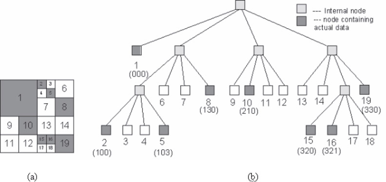
Figure 23.1(a) A binary 23 × 23 image and (b) its corresponding region quadtree. The location codes for the homogeneous codes are indicated in brackets.
Several linear representations of regional quadtrees have been proposed, but fixed length (FL), fixed length-depth (FD), and variable length (VL) versions have attracted most attention. We refer the interested reader to Reference 14 for details on these representations, while we concentrate on the FD representation. In this representation, each homogeneous node is represented by a pair of two codes, location code and level number. Location node C denotes the correct path to this node when traversing the Quadtree from its root till the appropriate leaf is reached and a level number L refers to the level at which the node is located. This makes up the FD linear implementation of Quadtree. The quadrants NW, NE, SW, and SE are represented as 0, 1, 2, and 3, respectively. The location codes for the homogeneous nodes of a quadtree are presented in Figure 23.1.
A persistent data structure (see Chapter 33) [15] is one in which a change to the structure can be made without eliminating the old version, so that all versions of the structure persist and can at least be accessed (the structure is said to be partially persistent) or even modified (the structure is said to be fully persistent). MVLQ is an example of a persistent data structure, in contrast to Linear Quadtree, a transient data structure. In MVLQ, each object in the database is labeled with a time for maintaining the past states. MVLQ couples time intervals with spatial objects in each node.
The leaf of the MVLQ contains the data records of the format:
where
C is the location code of the homogeneous node of the region quadtree,
L is the level of the region quadtree at which the homogeneous node is present,
T represents the time interval when the homogeneous node appears in the image sequence,
EndTime is transaction time when the homogeneous leaf node becomes historical.
The nonleaf nodes contain entries of the form [12]:
where
C′ is the smallest C recorded in that descendant node,
P′ is the time interval that expresses the lifespan of the latter node,
Ptr is a pointer to a descendant node,
StartTime is the time instant when the node was created.
The MVLQ structure after the insertion of image given in Figure 23.1a is given in Figure 23.2.
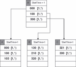
Figure 23.2MVLQ structure after the insertion of image given in Figure 23.1a.
In addition to the main memory structure of the MVLQ described earlier, it also contains two additional main memory substructures: Root*table and Depth First expression (DF-expression) of the last inserted object.
Root*table: MVLQ has one tree for each version of the data. Consequently, each version can be reached through its root which can be identified by the time interval of the version that it represents and a pointer to its location. If T′′ is the time interval of the root, given by T′′= [Ti, Tj), where i, j ∈ [1…n], i < j, and ptr′ is a pointer to the physical address of the root, then each record in the Root*table identifying a root is represented in the following form:
DF-expression of the last inserted object [12,16]: The purpose of Depth first expression (DF-expression) is to contain the prefetched location of the homogeneous nodes of last insert data object. The advantage of this storage is that when a new data object is being inserted, the stored information can be used to calculate the cost of deletions, insertions, and/or updates. If the DF-expression is not stored, then there is an input/output cost associated with locating the last insert object’s homogeneous nodes locations. The DF-expression is an array representation of preorder traversal of the last inserted object’s Quadtree.
23.2.1Insertion of an Object in MVLQ
The first step in insertion of a quadcode of a new object involves identifying the corresponding leaf node. If the corresponding leaf node is full, then a node overflow [12] occurs. Two possibilities may arise at this stage, and depending on the StartTime field of the leaf, a split may be initiated. If NC is the node capacity, k and c are integer constants (greater than zero), then the insertion is performed based on the algorithm presented in Figure 23.3.
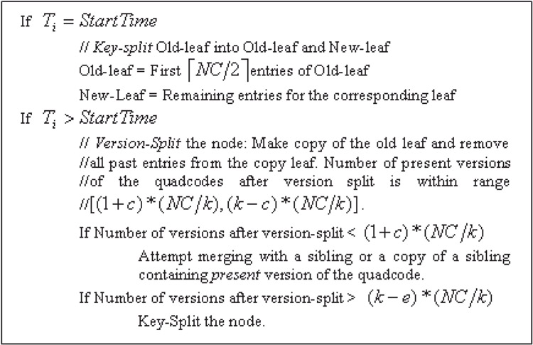
Figure 23.3Algorithm for an insertion of an object in MVLQ.
23.2.2Deletion of an Object in MVLQ
The algorithm for the deletion of an object from MVLQ is straightforward. If Ti = StartTime, then physical deletion occurs and the appropriate entry of the object is deleted from the leaf. If number of entries in the leaf < ⌈NC/k⌉ (threshold), then a node-underflow is handled as in B+ tree with an additional step of checking for a sibling’s StartTime for key redistribution. If Ti > StartTime, then logical deletion occurs and the temporal information of an entry between range ([Ti, * ), [Ti, Tj)) is updated. If an entry is logically deleted in a leaf with exactly ⌈NC/k⌉ present quadcode versions, then a version underflow [13] occurs that causes a version split of the node, copying the present versions of its quadcodes into a new node. After version split, the number of present versions of quadcodes is below (1 + e) ⌈NC/k⌉ and a merge is then attempted with a sibling or a copy of that sibling.
23.2.3Updating an Object in MVLQ
Updating a leaf entry refers to update of the field L (level) of the object’s code. This is implemented in a two-step fashion. First, a logical deletion of the entry is performed. Second, the new version is inserted in place of that entry through the steps outlined above.
In the previous section, a space-driven, MVLQ-based STDS was presented. In this section, we discuss a data-driven data structure that partitions the set of objects for efficient spatiotemporal representation.
Theodoridis et al. [17] have proposed a data structure termed 3D R-tree for indexing spatiotemporal information for large multimedia applications. The data structure is a derivation of R-trees (see Chapter 22) whose variants have been demonstrated to be an efficient indexing schema for high-dimensional spatial objects.
Theodoridis et al. [17] have adopted a set of operators defined by Papadias and Theodoridis [18] to represent possible topological–directional spatial relationships between two 2-dimensional objects. An anthology of 169 relationships Ri_j (i ∈ [1…13], j ∈ [1…13]) can represent a complete set of spatial operators. Figure 23.4 represents these relations. An interested reader can find a complete illustration of these topographical relationships in Reference 18. To represent the temporal relationships, a set of temporal operators defined in Reference 19 are employed. Any spatiotemporal relationships among objects can be found using these operators. For example, object Q to appear 7 seconds after the object P, 14 cm to the right and 2 cm down the right bottom vertex of object P can be represented as the following composition tuple:
where r13_13 is the corresponding spatial relationship, ( − 7 − > ) is the temporal relationship between the objects, v3 and v4 are the named vertices of the objects while (14, 2) are their spatial distances on the two axes.
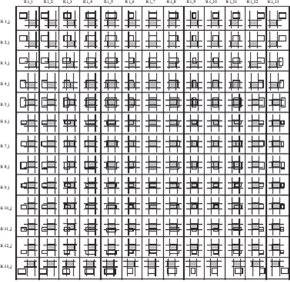
Figure 23.4Spatial relationships between two objects covering directional–topological information. (From M. Abdelguerfi et al., ACM-GIS, pp. 29–34, 2002.)
Theodoridis et al. have employed the following typical spatiotemporal relationships to illustrate their indexing schema [17]. These relationships can be defined as spatiotemporal operators.
•overlap_during(a, b): returns the catalogue of objects a that spatially overlap object b during its execution.
•overlap_before(a, b): returns the catalogue of objects a that spatially overlap object b and their execution terminates before the start of execution of b.
•above_during(a, b): returns the catalogue of objects a that spatially lie above object b during the course of its execution.
•above_before(a, b): returns the catalogue of objects a that spatially lie above object b and their execution terminates before the start of execution of b.
Spatial and temporal features of objects are typically identified by six dimensions (each spatiotemporal object can be perceived as a point in a six-dimensional space):
(x1, x2, y1, y2, t1, t2), where
(x1, x2): Projection of the object on the horizontal plane
(y1, y2): Projection of the object on the vertical plane
(t1, t2): Projection of the object on the time plane.
In a naïve approach, these object descriptors coupled by the object id (unique for the object that they represent) can be stored sequentially in a database. An illustration of such an organization is demonstrated in Figure 23.5.
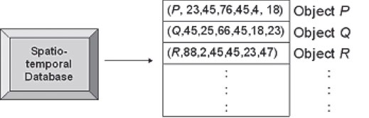
Figure 23.5Schema for sequential organization of spatiotemporal data.
Such a sequential schema has obvious demerits. Answering of spatial–temporal queries, such as one described earlier, would require a full scan of the data organization, at least once. As indicated before, most STB suffer from the curse of dimensionality and sequential organization of data exhibits this curse through depreciated performance, rather than reducing it.
In another schema, two indices can be maintained to store spatial and temporal components separately. Specifically, they can be organized as follows.
1.Spatial index: an index to store the size and coordinates of the objects in two dimensions;
2.Temporal index: a one-dimensional index for storing the duration and start/stop time for objects in one dimension.
R-trees and their variants have been demonstrated to be efficient for storing n-dimensional data. Generally speaking, they could be used to store the spatial space components in a 2D R-tree and temporal components in a 1D R-tree. This schema is better than sequential search, since a tree structure provides a hierarchical organization of data leading to a logarithmic time performance. More details on R-trees and its variants can be found in Chapter 22.
Although this schema is better than sequential searching, it still suffers from a limitation [17]. Consider the query overlap_during, which would require that both the indices (spatial 2D R-tree and temporal 1D R-tree) are searched individually (in the first phase) and then the intersection of the recovered answer sets from each of the indices is reported as the index’s response to the query. Access to both the indices individually and then postintersection can cumulatively be a computationally expensive procedure, especially when each of these indices is dense. Spatial joins [17,20] have been proposed to handle queries on two indexes, provided these indexing schemas adopt the same spatial data structure. It is not straightforward to extend these to handle joins in two varieties of spatial data structures. Additionally, there might be possible inherent relationships between the spatial descriptors and the temporal descriptors resident in two different indexes which can be learned and exploited for enhanced performance. Arranging and searching these descriptors separately may not be able to exploit these relationships. Hence, a unified framework is needed to present spatiotemporal components preferably in a same indexing schema.
Before we proceed further, let us briefly discuss the similarity search procedure in R-trees. In R-trees, minimum bounding boxes (MBB or minimum bounding rectangles in two dimensions) are used to assign geometric descriptors to objects for similarity applications, especially in data mining [21]. The idea behind the usage of MBB in R-trees is the following. If two objects are disjoint, then their MBBs should be disjoint, and if two objects overlap, then their MBB should definitely overlap. Typically, a spatial query on an MBB-based index involves the following steps.
(1) Searching the index: This step is used to select the answer and some possible false alarms from a given data set, ignoring those records that cannot possibly satisfy the query criterion. (2) Dismissals of false alarms: The input to this step is the resultant of the index searching step. In this step, the false alarms are eliminated to identify correct answers, which are reported as the query response. Designing an indexing schema for a multimedia application requires design of a spatiotemporal indexing structure to support spatiotemporal queries. Consider the following scenario.
Example 23.1
An application starts with a video clip A located at point (1,7) relative to the application origin Θ. After 2 minutes, an image B appears inside A with 1 unit above its lower horizontal edge and 3 units after its left vertical edge. B disappears after 2 minutes of its presence, while A continues. After 2 minutes of B’s disappearance, an text window C appears 3 units below the lower edge of A and 4 units to the right of left edge of it. A then disappears after 1 minute of C’s appearance. The moment A disappears, a small image D appears 2 units to the right of right edge of C and 3 units above the top edge of C. C disappears after 2 minutes of D’s appearance. As soon as C disappears, a text box E appears 2 units below the lower edge of D and left aligned with it. E lasts for 4 minutes after which it disappears. D disappears 1 minute after E’s disappearance. The application ends with D’s disappearance. The spatial layout of the above scenario is presented in Figure 23.6a and the temporal layout is presented in Figure 23.6b.
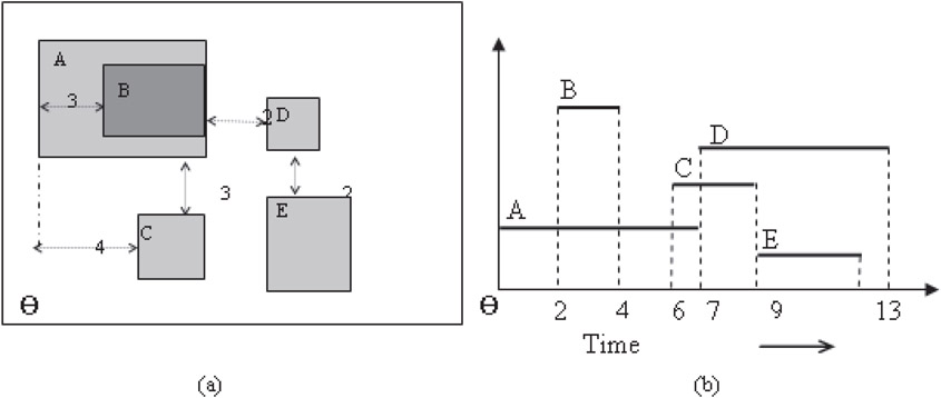
Figure 23.6(a) Spatial layout of the multimedia database and (b) temporal layout of the multimedia database.
A typical query that can be posed on such a database of objects described earlier is “Which objects overlap the object A during its presentation?” In Reference 17, the authors have proposed a unified schema to handle queries on an STB, such as the one stated above. The schema amalgamates the spatial and temporal components in a single data structure such as R-trees to exhibit advantages and performance gains over the other schemas described earlier. This schema amalgamates need of spatial joins on two spatial data structures besides aggregating both attributes under a unified framework. The idea for representation of spatiotemporal attributes is as follows. If an object which initially lies at point (xa, ya) during time [ta, tb) and at (xb, yb) during [tb, tc), it can be modeled by two lines and . These lines can be presented in a hierarchical R-tree index in three dimensions. Figure 23.7 presents the unified spatial–temporal schema for the spatial and temporal layouts of the example presented above.
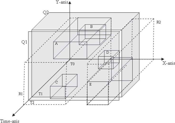
Figure 23.7A unified R-tree-based schema for storing spatial and temporal components.
23.3.1Answering Spatiotemporal Queries Using the Unified Schema
Answering queries on the above presented unified schema is similar to handling similarity queries using R-trees. Consider the following queries [17]:
Query 1: “Find all the objects on the screen at time T2” (spatial layout query). This query can be answered by considering a rectangle Q1 (Figure 23.7) intersecting the time axis at exactly one point, T2.
Query 2: “Find all the objects and their corresponding temporal duration between the time interval (T0, T1)” (temporal layout query). This query can be answered by considering a box Q2 (Figure 23.7) intersecting the time axis between the intervals (T0, T1).
After we have obtained the objects enclosed by the rectangle Q1 and box Q2, these objects are filtered (in main memory) to obtain the answer set.
Query 3: “Find all the objects and their corresponding spatial layout at time T = 3 minutes.” This query can be answered by looking at the screenshot of spatial layout of objects that were present at the given instant of time. The resultant would be the list of objects and their corresponding spatial descriptors. The response to this query is given in Figure 23.8a.
Query 4: Find the temporal layout of all the objects between the time interval (T1 = 2, T2 = 9). This query can be answered by drawing a rectangle on the unified index with dimensions (Xmax − 0) × (Ymax − 0) × (T2 − T1). The response of the query is shown in Figure 23.8b.
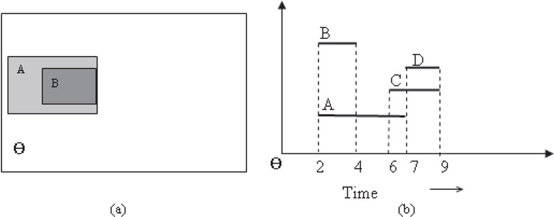
Figure 23.8(a) Response to Query 3 and (b) response to Query 4.
23.3.2Spatiotemporal Query Types
Here, we consider some major query types that are commonly performed on spatiotemporal data. Existing algorithms for these are mostly predictive in nature [9].
•Range queries [22,23]: This has a query range R and a future time t, and requests about the objects expected to be inside R after time t. This utilizes a mobility model that is based on a time parameterized bounding rectangle as a moving region that intersects or otherwise, a moving circle that represents a range query.
•K-nearest-neighbor queries [23,24]: This has a location point P, a future time t, and requests about the K objects expected to be closest to P after time t. Two algorithms, RangeSearch and KNNSearchBF, work by traversing spatiotemporal index tree (TPR/TPR*-tree) to find the nodes that intersect with the query circular region for Range and KNN queries, respectively.
•Reverse-nearest-neighbor queries [23,25]: Contrary to the predictive KNN query, predictive reverse-nearest-neighbor query finds out the objects expected to have the query region as their nearest neighbor.
•Aggregate queries [26]: This type has a query region R, future time t, and requests about the number of objects N predicted to be inside R after time t. Sun et al. [26] present a comprehensive technique that employs adaptive multidimensional histogram (AMH), historical synopsis, and stochastic method to provide approximate answers for aggregate spatiotemporal queries for the future, in addition to the past, and the present.
•Continuous queries [27,28]: Continuous query Q, mostly server-side algorithm that is stored until the end of its life, could be any of the above discussed types but with the additional condition that it needs to be continuously reevaluated many times throughout its life in the underlying system. The rate of reevaluation depends on the time gap, tgap between each two consecutive reported answers specified in the received query Q.
23.3.3Performance Analysis of 3D R-Trees
Theodoridis et al. [17] analyzed the performance of the proposed R-trees using the expected retrieval cost metric that they presented in Reference 15. An interested reader is referred to References 17 and 29 for details on this metric. Based on the analytical model of this metric, it is asserted that one can estimate the retrieval cost of an overlap query based on the information attainable from the query window and data set only. In the performance analysis, it was demonstrated that since the expected retrieval cost metric expresses the expected performance of R-trees on overlapping queries, the retrieval of spatiotemporal operators using R-trees is cost equivalent to the cost of retrieval of an overlap query using an appropriate query window Q. Rigorous analysis with 10,000 objects asserted the following conclusions as described in Reference 17:
1.For the operators with high selectivity (overlap, during, overlap_during), the proposed 3D R-trees outperformed sequential search at a level of 1 to 2 orders of magnitude.
2.For operators with low selectivity (above, before, above_before), the proposed 3D R-trees outperformed sequential search by factors ranging between 0.25 and 0.50 fraction of the sequential cost.
23.3.4Handling Queries with Open Transaction Times
In the previous section although 3D R-trees were demonstrated to be very efficient compared to sequential search, it suffers from a limitation. The transaction times presented as creation and termination time of an object are expected to be known a priori before they can be stored and queried from the index. However, in most practical circumstances, the duration of existence of an object is not known. In other words, when the object is created, all we know is that it would remain valid until changed. The concept of until changes is a well-discussed issue [30,31]. Data structures like R-trees and also its modified form of 3D R-tree are typically not capable of handling such queries having open transaction times. In the following section, we discuss two STDS capable of handling queries with open transaction times.
Nascimento et al. [31] have proposed a solution to the problem of handling objects with open transaction times. The idea is to split the indexing of these objects into two parts: one for two-dimensional points and other for three-dimensional lines. Two-dimensional points store the spatial information about the objects and their corresponding start time. Three-dimensional lines store the historical information about the data. Once the “started” point stored in 2D R-tree becomes closed, a corresponding line is constructed to be stored in the 3D R-tree and the point entry is deleted from the 2D R-tree. It should be understood that both trees are expected to be searched depending on the timestamp at which the query is posed. If the end times for each of the spatial points is known a priori, then the need of a 2D can be completely eliminated reducing the structure to a 3D R-tree.
One possible way to index spatiotemporal data is to build one R-tree for each timestamp, which is certainly space inefficient. The demerit of 2 + 3 R-tree is that it requires two stores to be searched to answer a query. The HR-tree [32] or Historical R-tree “compresses” multiple R-trees, so that R-tree nodes which are common in two timestamps are shared by the corresponding R-trees. The main idea is based on the expectation that a vast majority of indexed points do not change their positions at every timestamp. In other words, it is reasonable to expect that a vast majority of spatial points will “share” common nodes in respective R-trees. The HR-tree exploits this property by keeping a “logical” linkage to a previously present spatial point if it is referenced again in the new R-tree. Consider two R-trees in Figures 23.9 and 23.10 at two different timestamps (T0, T1). An HR-tree for these R-trees is given in Figure 23.11.
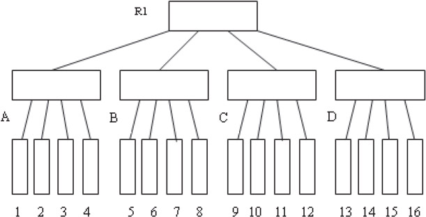
Figure 23.9An R-tree at time T0.
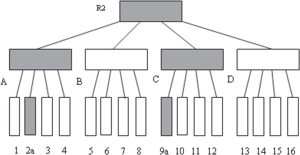
Figure 23.10An R-tree at time T1. The modified nodes are in dark boxes.
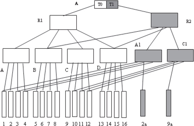
Figure 23.11The HR-tree.
Recently, Ni and Ravishankar [33] proposed the PA-tree as an indexing scheme for historical trajectory data. PA-tree is a parametric space indexing method that uses approximating sequence of movement functions with single continuous polynomial approximations, and demonstrated how this could support both offline and online query processing of historical trajectories. Their work showed that although existing schemes such as MVR-trees and SETI are faster for index construction and timestamp queries, PA-trees are an order of magnitude faster to construct and incur lower I/O cost for spatiotemporal range queries which makes it an excellent choice for both offline and online processing of historical trajectories.
The MV3R-tree was proposed by Tao and Papadias [34] and is demonstrated to process timestamp and interval queries efficiently. Timestamp queries discover all objects that intersect a window query at a particular timestamp. On the other hand, interval queries include multiple timestamps in the discovered response. While the spatial data structures proposed before have been demonstrated [17,34] to be suitable for either of these queries (or a subset of it), none of them have been established to process both timestamp and interval queries efficiently. MV3R-tree has addressed limitations in terms of efficiency of the above trees in handling both of these queries. MV3R-tree consists of a multiversion R-tree (MVR-tree) and an auxiliary 3D R-tree built on the leaves of the MVR-tree. Although the primary motivation behind the development of MV3R-tree is MVBT [13] (which are extended from B+ trees), they are significantly different from these versions. Before we proceed further, let us understand the working of an MVBT.
A typical entry of an MVBT takes the following form: < id, timestart, timeend, P >. For nonleaf nodes, timestart and timeend are the minimum and maximum values, respectively, in this node and P is a pointer to the next level node. For a leaf node, the timestamps timestart and timeend indicate when the object was inserted and deleted from the index and pointer P points to the actual record with a corresponding id value. At time timecurrent, the entry is said to be alive if timestart < timecurrent, otherwise dead [34]. There can be multiple roots in an MVBT, where each root has a distinguishing time range it represents. A search on the tree begins at identifying the root within which the timestamp of the query belongs. The search is continued based on the id, timestart, and timeend. A weak version condition specifies that for each node, except the root, at least K.T entries are alive at time t, where K is the node capacity and T is the tree parameter. This condition ensures that entries alive at the identical timestamps are in a majority of the cases assembled together to allow easy timestamp queries.
3D R-trees are very space efficient and can handle long interval queries efficiently. However, timestamp and short-interval queries using 3D R-trees are expensive. In addition to this, 3D R-trees do not include a methodology such as the weak version condition to ensure that each node has a minimum number of live entries at a given timestamp. HR-trees [32], on the other hand, maintain an R-tree (or its derivative) for each timestamp and the timestamp query is directed to the corresponding R-tree to be searched within it. In other words, the query disintegrates into an ordinary window query and is handled very efficiently. However, in case of an interval query, several timestamps should search the corresponding trees of all the timestamps constituting the interval. The original work in HR-tree did not present a schema for handling interval queries; however, Tao and Papadias [34] have proposed a solution to this problem by the use of negative and positive pointers. The performance of this schema is then compared with MV3R-tree in Reference 34. It is demonstrated that MV3R-trees outperform HR-trees and 3D R-trees even in extreme cases of only timestamp and interval-based queries.
Multiversion 3D R-trees (MV3R-trees) combine a multiversion R-tree (MVR-tree) and a small auxiliary 3D R-tree built on the leaf nodes of the MVR-tree as shown in Figure 23.12. MVR-trees maintain multiple R-trees and have entries of the form < MBR, timestart, timeend, P > , where MBR refers to minimum bounding rectangle and other entries are similar to B+ trees. An example of a 3D visualization of an MVR-tree of height 2 is shown in Figure 23.13. The tree consists of Object cubes (A–G), leaf nodes (H–J) and root of the tree K. Detailed algorithms for insertion and deletion in these trees are provided in Reference 34. Timestamp queries can be answered efficiently using MVR-trees. An auxiliary 3D R-tree is built on the leaves of the MVR-tree in order to process interval queries. It is suggested that for a moderate node capacity, the number of leaf nodes in an MVR-tree is much lower than the actual number of objects, hence this tree is expected to be small compared to a complete 3D R-tree.
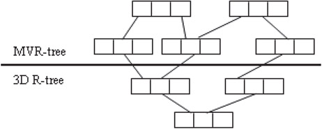
Figure 23.12An MV3R-tree.
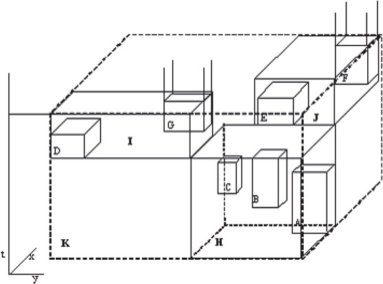
Figure 23.13A 3D visualization of MVR-tree.
Performance analysis has shown that the MV3R-tree offers better trade-off between query performance and structure size than the HR-tree and 3D R-tree. For typical situations where workloads contain both timestamp and interval queries, MV3R-trees outperform HR-trees and 3D R-trees significantly. The incorporation of the auxiliary 3D R-tree not only accelerates interval queries but also provides flexibilities toward other query processing, such as spatiotemporal joins.
23.7Indexing Structures for Continuously Moving Objects
Continuously moving objects pose new challenges to indexing technology for large databases. Sources for such data include GPS systems, wireless networks, air-traffic controls, and so on. In the previous sections, we have outlined some indexing schemas that could efficiently index spatiotemporal data types but some other schemas have been developed specifically for answering predictive queries in a database of continuously moving objects. In this section, we discuss an assortment of such indexing schemas.
Databases of continuously moving objects have two kinds of indexing issues: storing the historical movements in time of objects and predicting the movement of objects based on previous positional and directional information. Such predictions can be made more reliably for a future time Tf, not far from the current timestamp Tf. As Tf increases, the predictions become less and less reliable since the change of trajectory by a moving object results in inaccurate prediction. Traditional indexing schemas such as R*-trees are successful in storing multidimensional data points but are not directly useful for storing moving objects. An example [35] of such kind of system is shown in Figure 23.14. For simplicity, a two-dimensional space is illustrated, but practical systems can have larger dimensions. First part of the figure shows multiple objects moving in different directions. If traditional R*-trees are used for indexing these data, the MBB for the leaf level of the tree are demonstrated in Figure 23.14b. But these objects might be following different trajectories (as shown by arrows in Figure 23.14a) and at subsequent timestamps, the leaf level MBB might change in size and position, as demonstrated in Figure 23.14c and d.
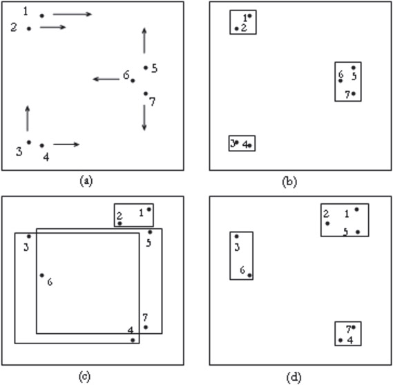
Figure 23.14Moving data points and their leaf-level MBBs at subsequent points.
Since traditional indexing methods are not designed for such kind of applications, some novel indexing schemas are described in References 35–38 to handle such data types and queries imposed on them.
Saltenis et al. [35] proposed TPR-tree, an acronym for Time-Parameterized R*-tree, based on the underlying principles of R-tree. TPR-tree indexes the current and future anticipated positions of moving objects in one, two, and three dimensions. The basic algorithms of R*-trees are employed for TPR-tree with a modification that the leaf and nonleaf minimum bounding rectangles are now augmented with velocity vectors for these rectangles. The velocity vector for an edge of the rectangle is chosen so that the object remains inside the moving rectangle. TPR-tree can typically handle the following three types of queries:
•Timeslice Query: A query Q specified by hyperrectangle R located at time point t.
•Window Query: A query Q specified by hyperrectangle R covering an interval from [Ta,Tb].
•Moving Query: A query Q specified by hyperrectangles Ra and Rb at different times Ta and Tb, forming a trapezoid.
Figure 23.15 shows objects o1, o2, o3, and o4 moving in time. The trajectories of these objects are shifting, as shown in the figure. The three types of queries as described earlier are illustrated in this figure. Q0 and Q1 are timeslice queries, Q2 and Q3 are window queries, and Q4 is a moving query.
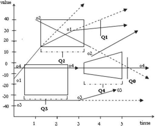
Figure 23.15Types of queries on one-dimensional data.
The structure of TPR-tree is very similar to R*-tree with leaves consisting of position and pointer of the moving object. The nodes of the tree consist of pointers to subtree and bounding rectangles for the entries in subtree. TPR-trees store the moving objects as linear function of time with time-parameterized bounding rectangles. The index does not consist of points and rectangles for timestamp older than current time. TPR-tree differs from the R*-trees in how its insertion algorithms group points into nodes. While in R*-trees, the heuristics of the minimized area, overlap, and margin of bounding rectangles are used to assign points to the nodes of the tree, in case of TPR-trees these heuristics are replaced by their respective integrals, which are representative of their temporal components. Given an objective function F(t), the following integral is expected to be minimized [35].
where tc is the current time and H is the time horizon.
The objective function can be area or perimeters of the bounding rectangles, or could represent the overlap between these rectangles. Figure 23.16 represents a bounding interval and a query in the TPR-tree. The area of the shaded region in Figure 23.16 represents the time integral of the length of the bounding interval.
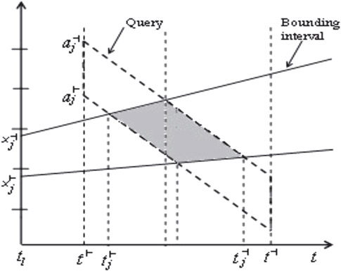
Figure 23.16A bounding interval and a query imposed on the TPR-tree.
Saltenis et al. [35] compared the performance of TPR-trees with load-time bounding rectangles, TPR-tree with update-time bounding rectangles, and R-tree with a set of experiments with varying workloads. The results demonstrated that TPR-tree outperforms other approaches by considerable improvement. It was also demonstrated that TPR-tree does not degrade severely in performance with increasing time and it can be tuned to take advantage of a specific update rate.
Saltenis and Jensen [36] proposed REXP-tree as a balanced, multiway tree with a structure of R*-tree. REXP-tree is an improvement over TPR-tree, assuming that some objects used in indexing expires after a certain period. These trees can handle realistic scenario where certain objects are no longer required, that is when they expire. By removing the expired entries and recomputing bounding rectangles, the index organizes itself to handle subsequent queries efficiently. This tree structure finds its application where the objects do not report their positions for a certain period, possibly implying that they are no more interested in the service.
The index structure of REXP-tree differs from TPR-tree in insertion and deletion algorithms for disposing the expired nodes. REXP-tree uses a “lazy strategy” for deleting the expired entries. Another possible strategy is scheduled deletion of entries in TPR-trees. During the search, insertion, and deletion operations, only the live entries are searched and expired entries are physically removed when the content of the node is modified and is written to the disk. Whenever an entry in internal node is deleted, the entire subtree is reallocated. The performance results demonstrated in Reference 36 show that choosing the right bounding rectangles and corresponding algorithms for grouping entries is not straightforward and depends on the characteristics of the workloads.
Procopiuc et al. [37] propose a Spatio-Temporal Self-Adjusting R-tree or STAR-tree. STAR-tree indexing schema is similar to TPR trees with few differences. Specifically, STAR-tree groups point according to their current locations and may result in points moving with different velocities being included in the same rectangle. Scheduled events are used to regroup points to control the growth of such bounding rectangles. It improves the structure of TPR-tree by self-adjusting the index, whenever index performance degrades. Intervention of user is not needed for adjustment of the index and the query time is kept low even without continuously updating the index by positions of the objects. STAR-tree does not need periodic rebuilding of indexing and estimation of time horizon. It provides trade-offs between storage and query performance and between time spent in updating the index and in answering queries. STAR-tree can handle not only the timeslice and range queries as those handled by TPR-trees but also nearest neighbor queries for continuously moving objects.
TPR*-tree proposed by Tao et al. [38] is an optimized spatiotemporal indexing method for predictive queries. TPR-tree, described in the previous section, does not propose an analytical model for cost estimation and query optimization and quantification of its performance. TPR*-tree assumes a probabilistic model that accurately estimates the number of disk accesses in answering a window query in a spatiotemporal index. Tao et al. [38] investigate the optimal performance of any data partition index using the proposed model.
The TPR*-tree improves the performance of TPR-tree by employing a new set of insertion and deletion algorithms that minimize the average number of node accesses for answering a window query, whose MBB uniformly distributes in the data space. The static point interval query with the following constraints has been optimized [38] using the TPR*-tree:
•MBB has a length |QR| = 0 on each axis.
•Velocity bounding rectangle is {0,0,0,0}.
•Query interval QI = [0, H], where H is the horizon parameter.
It is demonstrated that the above choice of parameters leads to nearly optimal performance independently of the query parameters. The experiments have also shown that TPR*-trees significantly outperform the conventional TPR-tree under all conditions.
1.B.-U. Pagel, F. Korn, C. Faloutsos, “Deflating the Dimensionality Curse using Multiple Fractal Dimensions,” In 16th International Conference on Data Engineering (ICDE), San Diego, CA, 2000.
2.S. Ke, J. Gong, S. Li, Q. Zhu, X. Liu, Y. Zhang, “A Hybrid Spatio-Temporal Data Indexing Method for Trajectory Databases,” Sensors, Vol. 14, 2014, pp. 12990–13005.
3.C. S. Jensen, J. Clifford, R. Elmarsi et al., “A Consensus Glossary of Temporal Database Concepts,” SIGMOD Record, 23 (1), pp. 52–64, 1994.
4.M. Abdelguerfi, J. Givaudan, K. Shaw, R. Ladner, “The 2–3TR-Tree, a Trajectory-Oriented Index Structure for Fully Evolving Valid-Time Spatio-Temporal Datasets,” Proceedings of the 10th ACM international Symposium on Advances in Geographic Information Systems (GIS ’02). ACM, New York, NY, USA, pp. 29–34, 2002. https://dl.acm.org/citation.cfm?id=585155
5.M. Mokbel, T. Ghanem, W. Aref, “Spatio-Temporal Access Methods,” IEEE Data Engineering Bulletin, Vol. 26, 2003, pp. 40–49.
6.V. Chakka, A. Everspaugh, J. Patel, “Indexing Large Trajectory Data Sets with SETI,” In Proceedings of the 2003 CIDR Conference, Asiloma, USA, 2003.
7.L.-V. Nguyen-Dinh, W. G. Aref, M. Mokbel, “Spatio-Temporal Access Methods: Part 2 (2003–2010),” Purdue University Libraries—Purdue e-Pubs: Cyber Center Publications, Paper 19, 2010.
8.Z. He, M. J. Kraak, O. Huisman, X. Ma, J. Xiao, “Parallel Indexing Technique for Spatio-Temporal Data,” ISPRS Journal of Photogrammetry and Remote Sensing, Vol. 78, 2013, pp. 116–128.
9.A. M. Hendawi, M. F. Mokbel, “Predictive Spatio-Temporal Queries: A Comprehensive Survey and Future Directions,” In ACM SIGSPATIAL MobiGIS’12, Redondo Beach, CA, 2012.
10.J. Dittrich, L. Blunschi, M. A. V. Salles, “MOVIES: Indexing Moving Objects by Shooting Index Images,” International Journal on Advances of Computer Science for Geographic Information Systems, GeoInformatica, Vol. 15, No. 4, pp. 727–767, 2011.
11.J. D. L. Blunschi, M. A. V. Salles, “Indexing Moving Objects Using Short-Lived Throwaway Indexes,” In Proceedings of the 11th International Symposium on Advances in Spatial and Temporal Databases, July 08–10, Aalborg, Denmark, 2007. Doi: 10.1007/978-3-642-02982-0_14.
12.T. Tzouramanis, M. Vassilakopoulos, Y. Manolopoulos, “Multiversion linear quadtree for spatiotemporal Data,” In Proceedings 4th East-European Conference on Advanced Databases and Information Systems (ADBIS-DASFAA’00), 279–292, Prague, Czech Republic, 2000.
13.B. Becker, S. Gschwind, T. Ohler, B. Seeger, P. Widmayer, “An Asymptotically Optimal Multiversion B-tree,” The VLDB Journal, Vol. 5, pp. 264–275, 1996.
14.H. Samet, The Design and Analysis of Spatial Data Structures, Addison-Wesley, Reading, MA, 1990.
15.J. R. Driscoll, N. Sarnak, D. D. Sleator, R. E. Tarjan, “Making Data Structures Persistent,” Journal of Computer and System Sciences, Vol. 38, pp. 86–124, 1989.
16.E. Kawaguchi, T. Endo, “On a Method of Binary Picture Representation and its Application to Data Compression,” IEEE Transactions on Pattern Analysis and Machine Intelligence, Vol. 2, No. 1, pp. 27–35, 1980.
17.Y. Theodoridis, M. Vazirgiannis, T. Sellis, “Spatio-Temporal Indexing for Large Multimedia Applications,” In Proceedings of the Third IEEE International Conference on Multimedia Computing and Systems, Hiroshima, Japan, pp. 441–448, 1996.
18.D. Papadias, Y. Theodoridis, “Spatial Relations, Minimum Bounding Rectangles, and Spatial Data Structures,” International Journal of Geographic Information Systems, Vol. 11, No. 2, 1997.
19.M. Vazirgiannis, Y. Theodoridis, T. Sellis, “Spatio-Temporal Composition in Multimedia Applications,” Technical Report KDBSLAB-TR-95-09, Knowledge, Database Systems Laboratory, National Technical University of Athens, 1995.
20.M. G. Martynov, “Spatial Joins and R-trees.” In J. Eder, L.A. Kalinichenko (eds.), Advances in Databases and Information Systems. Workshops in Computing. Springer, London, 1996.
21.Y. Theodoridis, D. Papadias, “Range Queries Involving Spatial Relations: A Performance Analysis,” In A.U. Frank, W. Kuhn (eds.), Spatial Information Theory A Theoretical Basis for GIS. COSIT 1995. Lecture Notes in Computer Science, vol 988. Springer, Berlin, Heidelberg, 1995.
22.H. Jeung, M. L. Yiu, X. Zhou, C. S. Jensen, “Path Prediction, Predictive Range Querying in Road Network Databases,” VLDB Journal, Vol. 19, pp. 585–602, 2010.
23.R. Zhang, H. V. Jagadish, B. T. Dai, K. Ramamohanarao, “Optimized Algorithms for Predictive Range and KNN Queries on Moving Objects,” Information Systems, Vol. 35, pp. 911–932, 2010.
24.R. Benetis, C. S. Jensen, G. Karciauskas, S. Saltenis, “Nearest and Reverse Nearest Neighbor Queries for Moving Objects,” VLDB Journal, Vol. 15, pp. 229–249, 2006.
25.T. Xia, D. Zhang, “Continuous Reverse Nearest Neighbor Monitoring,” In Proceedings of the International Conference on Data Engineering, ICDE, Georgia, USA, 2006.
26.J. Sun, D. Papadias, Y. Tao, B. Liu, “Querying about the Past, the Present, and the Future in Spatio-Temporal,” In Proceedings of the International Conference on Data Engineering, ICDE, Massachusetts, USA, 2004.
27.J. Kang, M. F. Mokbel, S. Shekhar, T. Xia, D. Zhang, “Continuous Evaluation of Monochromatic and Bichromatic Reverse Nearest Neighbors,” In Proceedings of the International Conference on Data Engineering, ICDE, Istanbul, Turkey, 2007.
28.H. Wang, R. Zimmermann, W.-S. Ku, “Distributed Continuous Range Query Processing on Moving Objects,” In Proceedings of the International Conference on Database and Expert Systems Applications, DEXA, Krakow, Poland, 2006.
29.Y. Theodoridis, T. Sellis, “On the Performance Analysis of Multidimensional R-tree-based Data Structures,” Technical Report KDBSLABTR-95-03, Knowledge, Database Systems Laboratory, National Technical University of Athens, Greece, 1995.
30.J. Clifford, C. E. Dyreson, T. Isakowitz, C. S. Jensen, R. T. Snodgrass, “On the Semantics of “Now” in Databases,” ACM Transactions on Database Systems, 22, pp. 171–214, 1997.
31.M. Nascimento, R. Silva, Y. Theodoridis, “Evaluation of Access Structures for Discretely Moving Points,” In M.H. Böhlen, C.S. Jensen, and M. Scholl (eds.), Proceedings of the International Workshop on Spatio-Temporal Database Management (STDBM ’99), Springer-Verlag, London, UK, pp. 171–188, 1999.
32.M. Nascimento, J. Silvia, “Towards Historical Rtrees,” In Proceedings of the 1998 ACM symposium on Applied Computing (SAC ’98). ACM, New York, NY, USA, pp. 235–240, 1998.
33.J. Ni, C. V. Ravishankar, “Indexing Spatio-Temporal Trajectories with Efficient Polynomial Approximations,” IEEE Transactions on Knowledge and Data Engineering, Vol. 19, pp. 663–678, 2007.
34.Y. Tao, D. Papadias, “MV3R-Tree: A Spatio-Temporal Access Method for Timestamp and Interval Queries,” In Proceedings of the 27th International Conference on Very Large Data Bases, September 11–14, pp. 431–440, 2001.
35.S. Saltenis, C. Jensen, S. Leutenegger, M. Lopez, “Indexing the Positions of Continuously Moving Objects,” In Proceedings of the 19th ACM-SIGMOD International Conference on Management of Data, Dallas, TX, 2000.
36.S. Saltenis, C. S. Jensen, “Indexing of Moving Objects for Location-Based Services,” TimeCenter (2001), TR-63, 24 pages.
37.C.M. Procopiuc, P. K. Agarwal, S. Har-Peled, “STAR-Tree: An Efficient Self-Adjusting Index for Moving Objects,” In D.M. Mount, C. Stein (eds.), Revised Papers from the 4th International Workshop on Algorithm Engineering and Experiments (ALENEX ’02). Springer-Verlag, London, UK, pp. 178–193, 2002.
38.Y. Tao, D. Papadias, J. Sun, “The TPR*-Tree: An Optimized Spatio-Temporal Access Method for Predictive Queries,” Proceedings of the 29th International Conference on Very Large Data Bases, September 09–12, Berlin, Germany, pp. 790–801, 2003.