14. Randomized Dictionary Structures

In the last couple of decades, there has been a tremendous growth in using randomness as a powerful source of computation. Incorporating randomness in computation often results in a much simpler and more easily implementable algorithms. A number of problem domains, ranging from sorting to stringology, from graph theory to computational geometry, from parallel processing system to ubiquitous internet, have benefited from randomization in terms of newer and elegant algorithms. In this chapter we shall see how randomness can be used as a powerful tool for designing simple and efficient data structures. Solving a real-life problem often involves manipulating complex data objects by variety of operations. We use abstraction to arrive at a mathematical model that represents the real-life objects and convert the real-life problem into a computational problem working on the mathematical entities specified by the model. Specifically, we define Abstract Data Type (ADT) as a mathematical model together with a set of operations defined on the entities of the model. Thus, an algorithm for a computational problem will be expressed in terms of the steps involving the corresponding ADT operations. In order to arrive at a computer based implementation of the algorithm, we need to proceed further taking a closer look at the possibilities of implementing the ADTs. As programming languages support only a very small number of built-in types, any ADT that is not a built-in type must be represented in terms of the elements from built-in type and this is where the data structure plays a critical role. One major goal in the design of data structure is to render the operations of the ADT as efficient as possible. Traditionally, data structures were designed to minimize the worst-case costs of the ADT operations. When the worst-case efficient data structures turn out to be too complex and cumbersome to implement, we naturally explore alternative design goals. In one of such design goals, we seek to minimize the total cost of a sequence of operations as opposed to the cost of individual operations. Such data structures are said to be designed for minimizing the amortized costs of operations. Randomization provides yet another avenue for exploration. Here, the goal will be to limit the expected costs of operations and ensure that costs do not exceed certain threshold limits with overwhelming probability.

In this chapter we discuss about the Dictionary ADT which deals with sets whose elements are drawn from a fixed universe U and supports operations such as insert, delete and search. Formally, we assume a linearly ordered universal set U and for the sake of concreteness we assume U to be the set of all integers. At any time of computation, the Dictionary deals only with a finite subset of U. We shall further make a simplifying assumption that we deal only with sets with distinct values. That is, we never handle a multiset in our structure, though, with minor modifications, our structures can be adjusted to handle multisets containing multiple copies of some elements. With these remarks, we are ready for the specification of the Dictionary ADT.

Definition 14.1: (Dictionary ADT)

Let U be a linearly ordered universal set and S denote a finite subset of U. The Dictionary ADT, defined on the class of finite subsets of U, supports the following operations.

Insert (x, S) : For an x ∈ U, S ⊂ U, generate the set $S \cup {x}$ $S \cup {x}$ .

Delete (x, S) : For an x ∈ U, S ⊂ U, generate the set S − {x}.

Search (x, S) : For an x ∈ U, S ⊂ U, return TRUE if x ∈ S and return FALSE if x ∉ S.

Remark : When the universal set is evident in a context, we will not explicitly mention it in the discussions. Notice that we work with sets and not multisets. Thus, Insert (x,S) does not produce new set when x is in the set already. Similarly Delete (x, S) does not produce a new set when x ∉ S.

Due to its fundamental importance in a host of applications ranging from compiler design to data bases, extensive studies have been done in the design of data structures for dictionaries. Refer to Chapters 3 and 11 for data structures for dictionaries designed with the worst-case costs in mind, and Chapter 13 of this handbook for a data structure designed with amortized cost in mind. In Chapter 16 of this book, you will find an account of B-Trees which aim to minimize the disk access. All these structures, however, are deterministic. In this sequel, we discuss two of the interesting randomized data structures for Dictionaries. Specifically

•We describe a data structure called Skip Lists and present a comprehensive probabilistic analysis of its performance.

•We discuss an interesting randomized variation of a search tree called Randomized Binary Search Tree and compare and contrast the same with other competing structures.

14.2Preliminaries

In this section we collect some basic definitions, concepts and the results on randomized computations and probability theory. We have collected only the materials needed for the topics discussed in this chapter. For a more comprehensive treatment of randomized algorithms, refer to the book by Motwani and Raghavan [1].

14.2.1Randomized Algorithms

Every computational step in an execution of a deterministic algorithm is uniquely determined by the set of all steps executed prior to this step. However, in a randomized algorithm, the choice of the next step may not be entirely determined by steps executed previously; the choice of next step might depend on the outcome of a random number generator. Thus, several execution sequences are possible even for the same input. Specifically, when a randomized algorithm is executed several times, even on the same input, the running time may vary from one execution to another. In fact, the running time is a random variable depending on the random choices made during the execution of the algorithm. When the running time of an algorithm is a random variable, the traditional worst case complexity measure becomes inappropriate. In fact, the quality of a randomized algorithm is judged from the statistical properties of the random variable representing the running time. Specifically, we might ask for bounds for the expected running time and bounds beyond which the running time may exceed only with negligible probability. In other words, for the randomized algorithms, there is no bad input; we may perhaps have an unlucky execution.

The type of randomized algorithms that we discuss in this chapter is called Las Vegas type algorithms. A Las Vegas algorithm always terminates with a correct answer although the running time may be a random variable exhibiting wide variations. There is another important class of randomized algorithms, called Monte Carlo algorithms, which have fixed running time but the output may be erroneous. We will not deal with Monte Carlo algorithms as they are not really appropriate for basic building blocks such as data structures. We shall now define the notion of efficiency and complexity measures for Las Vegas type randomized algorithms.

Since the running time of a Las Vegas randomized algorithm on any given input is a random variable, besides determining the expected running time it is desirable to show that the running time does not exceed certain threshold value with very high probability. Such threshold values are called high probability bounds or high confidence bounds. As is customary in algorithmics, we express the estimation of the expected bound or the high-probability bound as a function of the size of the input. We interpret an execution of a Las Vegas algorithm as a failure if the running time of the execution exceeds the expected running time or the high-confidence bound.

Definition 14.2: (Confidence Bounds)

Let α, β and c be positive constants. A randomized algorithm A requires resource bound f(n) with

1.n − exponential probability or very high probability, if for any input of size n, the amount of the resource used by A is at most αf(n) with probability 1 − O(β⁻ⁿ), β > 1. In this case f(n) is called a very high confidence bound.

2.n − polynomial probability or high probability, if for any input of size n, the amount of the resource used by A is at most αf(n) with probability 1 − O(n^−c). In this case f(n) is called a high confidence bound.

3.n − log probability or very good probability, if for any input of size n, the amount of the resource used by A is at most αf(n) with probability 1 − O((log n)^−c). In this case f(n) is called a very good confidence bound.

4.high − constant probability, if for any input of size n, the amount of the resource used by A is at most αf(n) with probability 1 − O(β^−α), β > 1.

The practical significance of this definition can be understood from the following discussions. For instance, let A be a Las Vegas type algorithm with f(n) as a high confidence bound for its running time. As noted before, the actual running time T(n) may vary from one execution to another but the definition above implies that, for any execution, on any input, Pr(T(n) > f(n)) = O(n^−c). Even for modest values of n and c, this bound implies an extreme rarity of failure. For instance, if n = 1000 and c = 4, we may conclude that the chance that the running time of the algorithm A exceeding the threshold value is one in zillion.

14.2.2Basics of Probability Theory

We assume that the reader is familiar with basic notions such as sample space, event and basic axioms of probability. We denote as Pr(E) the probability of the event E. Several results follow immediately from the basic axioms, and some of them are listed in Lemma 14.1.

Lemma 14.1

The following laws of probability must hold:

1.Pr(ϕ) = 0

2.Pr(Ec) = 1 − Pr(E)

3.Pr(E1) ≤ Pr(E2) if E1 ⊆ E2

4.Pr(E1 ∪ E2) = Pr(E1) + Pr(E2) − Pr(E1∩ E2) ≤ Pr(E1) + Pr(E2)

Extending item 4 in Lemma 14.1 to countable unions yields the property known as sub additivity. Also known as Boole’s Inequality, it is stated in Theorem 14.1.

Theorem 14.1: (Boole’s Inequality)

$P r (\cup_{i = 1}^{\infty} E_{i}) \leq \sum_{i = 1}^{\infty} P r (E_{i})$ $P r (\cup_{i = 1}^{\infty} E_{i}) \leq \sum_{i = 1}^{\infty} P r (E_{i})$

A probability distribution is said to be discrete if the sample space S is finite or countable. If E = {e1, e2, …, e_k} is an event, $P r (E) = \sum_{i = 1}^{k} P r ({e_{i}})$ $P r (E) = \sum_{i = 1}^{k} P r ({e_{i}})$ because all elementary events are mutually exclusive. If |S| = n and $P r ({e}) = \frac{1}{n}$ $P r ({e}) = \frac{1}{n}$ for every elementary event e in S, we call the distribution a uniform distribution of S. In this case,

\begin{array}{l} P r (E) = \sum_{e \in E} P r (e) \\ = \sum_{e \in E} \frac{1}{n} \\ = | E | / | S | \end{array}

$\begin{array}{l} P r (E) = \sum_{e \in E} P r (e) \\ = \sum_{e \in E} \frac{1}{n} \\ = | E | / | S | \end{array}$

which agrees with our intuitive and a well-known definition that probability is the ratio of the favorable number of cases to the total number of cases, when all the elementary events are equally likely to occur.

14.2.3Conditional Probability

In several situations, the occurrence of an event may change the uncertainties in the occurrence of other events. For instance, insurance companies charge higher rates to various categories of drivers, such as those who have been involved in traffic accidents, because the probabilities of these drivers filing a claim is altered based on these additional factors.

Definition 14.3: (Conditional Probability)

The conditional probability of an event E1 given that another event E2 has occurred is defined by Pr(E1/E2) (“Pr(E1/E2)” is read as “the probability of E1 given E2.”).

Lemma 14.2

$P r (E_{1} / E_{2}) = \frac{P r (E_{1} \cap E_{2})}{P r (E_{2})}$ $P r (E_{1} / E_{2}) = \frac{P r (E_{1} \cap E_{2})}{P r (E_{2})}$ , provided Pr(E2) ≠ 0.

Lemma 14.2 shows that the conditional probability of two events is easy to compute. When two or more events do not influence each other, they are said to be independent. There are several notions of independence when more than two events are involved. Formally,

Definition 14.4: (Independence of two events)

Two events are independent if Pr(E1 ∩ E2) = Pr(E1)Pr(E2), or equivalently, Pr(E1/E2) = Pr(E1).

Definition 14.5: (Pairwise independence)

Events E1, E2, …E_k are said to be pairwise independent if Pr(E_i ∩ E_j) = Pr(E_i)Pr(E_j), 1 ≤ i ≠ j ≤ n.

Given a partition S1, …, S_k of the sample space S, the probability of an event E may be expressed in terms of mutually exclusive events by using conditional probabilities. This is known as the law of total probability in the conditional form.

Lemma 14.3: (Law of total probability in the conditional form)

For any partition S1, …, S_k of the sample space S, $P r (E) = \sum_{i = 1}^{k} P r (E / S_{i}) P r (S_{i})$ $P r (E) = \sum_{i = 1}^{k} P r (E / S_{i}) P r (S_{i})$ .

The law of total probability in the conditional form is an extremely useful tool for calculating the probabilities of events. In general, to calculate the probability of a complex event E, we may attempt to find a partition S1, S2, …, S_k of S such that both Pr(E/S_i) and Pr(S_i) are easy to calculate and then apply Lemma 14.3. Another important tool is Bayes’ Rule.

Theorem 14.2: (Bayes’ Rule)

For events with non-zero probabilities,

1. $P r (E_{1} / E_{2}) = \frac{P r (E_{2} / E_{1}) P r (E_{1})}{P r (E_{2})}$ $P r (E_{1} / E_{2}) = \frac{P r (E_{2} / E_{1}) P r (E_{1})}{P r (E_{2})}$

2.If S1, S2, …, S_k is a partition, $P r (S_{i} / E) = \frac{P r (E / S_{i}) P r (S_{i})}{\sum_{j = 1} P r (E / S_{j}) P r (S_{j})}$ $P r (S_{i} / E) = \frac{P r (E / S_{i}) P r (S_{i})}{\sum_{j = 1} P r (E / S_{j}) P r (S_{j})}$

Proof. Part (1) is immediate by applying the definition of conditional probability; Part (2) is immediate from Lemma 14.3.■

14.2.3.1Random Variables and Expectation

Most of the random phenomena are so complex that it is very difficult to obtain detailed information about the outcome. Thus, we typically study one or two numerical parameters that we associate with the outcomes. In other words, we focus our attention on certain real-valued functions defined on the sample space.

Definition 14.6

A random variable is a function from a sample space into the set of real numbers. For a random variable X, R(X) denotes the range of the function X.

Having defined a random variable over a sample space, an event of interest may be studied through the values taken by the random variables on the outcomes belonging to the event. In order to facilitate such a study, we supplement the definition of a random variable by specifying how the probability is assigned to (or distributed over) the values that the random variable may assume. Although a rigorous study of random variables will require a more subtle definition, we restrict our attention to the following simpler definitions that are sufficient for our purposes.

A random variable X is a discrete random variable if its range R(X) is a finite or countable set (of real numbers). This immediately implies that any random variable that is defined over a finite or countable sample space is necessarily discrete. However, discrete random variables may also be defined on uncountable sample spaces. For a random variable X, we define its probability mass function (pmf) as follows:

Definition 14.7: (Probability mass function)

For a random variable X, the probability mass function p(x) is defined as p(x) = Pr(X = x), ∀x ∈ R(X).

The probability mass function is also known as the probability density function. Certain trivial properties are immediate, and are given in Lemma 14.4.

Lemma 14.4

The probability mass function p(x) must satisfy

1.p(x) ≥ 0, ∀x ∈ R(X)

2. $\sum_{x \in R (X)} p (x) = 1$ $\sum_{x \in R (X)} p (x) = 1$

Let X be a discrete random variable with probability mass function p(x) and range R(X). The expectation of X (also known as the expected value or mean of X) is its average value. Formally,

Definition 14.8: (Expected value of a discrete random variable)

The expected value of a discrete random variable X with probability mass function p(x) is given by $E (X) = μ_{X} = \sum_{x \in R (X)} x p (x)$ $E (X) = μ_{X} = \sum_{x \in R (X)} x p (x)$ .

Lemma 14.5

The expected value has the following properties:

1.E(cX) = cE(X) if c is a constant

2.(Linearity of expectation) E(X + Y) = E(X) + E(Y), provided the expectations of X and Y exist

Finally, a useful way of computing the expected value is given by Theorem 14.3.

Theorem 14.3

If R(X) = {0, 1, 2, …}, then $E (X) = \sum_{i = 1}^{\infty} P r (X \geq i)$ $E (X) = \sum_{i = 1}^{\infty} P r (X \geq i)$ .

Proof.

\begin{matrix} E (X) & = & \sum_{i = 0}^{\infty} i P r (X = i) \\ = & \sum_{i = 0}^{\infty} i (P r (X \geq i) - P r (X \geq i + 1)) \\ = & \sum_{i = 1}^{\infty} P r (X \geq i) \end{matrix}

$\begin{matrix} E (X) & = & \sum_{i = 0}^{\infty} i P r (X = i) \\ = & \sum_{i = 0}^{\infty} i (P r (X \geq i) - P r (X \geq i + 1)) \\ = & \sum_{i = 1}^{\infty} P r (X \geq i) \end{matrix}$

■

14.2.4Some Basic Distributions

14.2.4.1Bernoulli Distribution

We have seen that a coin flip is an example of a random experiment and it has two possible outcomes, called success and failure. Assume that success occurs with probability p and that failure occurs with probability q = 1 − p. Such a coin is called p-biased coin. A coin flip is also known as Bernoulli Trial, in honor of the mathematician who investigated extensively the distributions that arise in a sequence of coin flips.

Definition 14.9

A random variable X with range R(X) = {0, 1} and probability mass function Pr(X = 1) = p, Pr(X = 0) = 1 − p is said to follow the Bernoulli Distribution. We also say that X is a Bernoulli random variable with parameter p.

14.2.4.2Binomial Distribution

Let $(\begin{matrix} n \\ k \end{matrix})$ $(\begin{matrix} n \\ k \end{matrix})$ denote the number of k-combinations of elements chosen from a set of n elements. Recall that $(\begin{matrix} n \\ k \end{matrix}) = \frac{n!}{k! (n - k)!}$ $(\begin{matrix} n \\ k \end{matrix}) = \frac{n!}{k! (n - k)!}$ and $(\begin{matrix} n \\ 0 \end{matrix}) = 1$ $(\begin{matrix} n \\ 0 \end{matrix}) = 1$ since 0! = 1. $(\begin{matrix} n \\ k \end{matrix})$ $(\begin{matrix} n \\ k \end{matrix})$ denotes the binomial coefficients because they arise in the expansion of (a + b)n.

Define the random variable X to be the number of successes in n flips of a p-biased coin. The variable X satisfies the binomial distribution. Specifically,

Definition 14.10: (Binomial distribution)

A random variable with range R(X) = {0, 1, 2, …, n} and probability mass function

P r (X = k) = b (k, n, p) = (\begin{matrix} n \\ k \end{matrix}) p^{k} q^{n - k}, f o r k = 0, 1, \dots, n

$P r (X = k) = b (k, n, p) = (\begin{matrix} n \\ k \end{matrix}) p^{k} q^{n - k}, f o r k = 0, 1, \dots, n$

satisfies the binomial distribution. The random variable X is called a binomial random variable with parameters n and p.

Theorem 14.4

For a binomial random variable X, with parameters n and p, E(X) = np and V ar(X) = npq.

14.2.4.3Geometric Distribution

Let X be a random variable X denoting the number of times we toss a p-biased coin until we get a success. Then, X satisfies the geometric distribution. Specifically,

Definition 14.11: (Geometric distribution)

A random variable with range R(X) = {1, 2, …, ∞} and probability mass function Pr(X = k) = q^k−1p, for k = 1, 2, …, ∞ satisfies the geometric distribution. We also say that X is a geometric random variable with parameter p.

The probability mass function is based on k − 1 failures followed by a success in a sequence of k independent trials. The mean and variance of a geometric distribution are easy to compute.

Theorem 14.5

For a geometrically distributed random variable X, $E (X) = \frac{1}{p}$ $E (X) = \frac{1}{p}$ and $V a r (X) = \frac{q}{p^{2}}$ $V a r (X) = \frac{q}{p^{2}}$ .

14.2.4.4Negative Binomial distribution

Fix an integer n and define a random variable X denoting the number of flips of a p-biased coin to obtain n successes. The variable X satisfies a negative binomial distribution. Specifically,

Definition 14.12

A random variable X with R(X) = {0, 1, 2, …} and probability mass function defined by

$\begin{aligned} P r (X = k) & = (\begin{matrix} k - 1 \\ n - 1 \end{matrix}) p^{n} q^{k - n} i f k \geq n \\ = 0 i f 0 \leq k < n \end{aligned}$ $\begin{aligned} P r (X = k) & = (\begin{matrix} k - 1 \\ n - 1 \end{matrix}) p^{n} q^{k - n} i f k \geq n \\ = 0 i f 0 \leq k < n \end{aligned}$	(14.1)

is said to be a negative binomial random variable with parameters n and p.

Equation 14.1 follows because, in order for the nth success to occur in the kth flip there should be n − 1 successes in the first k − 1 flips and the kth flip should also result in a success.

Definition 14.13

Given n identically distributed independent random variables X1, X2, …, X_n, the sum

S_{n} = X_{1} + X_{2} + \dots + X_{n}

$S_{n} = X_{1} + X_{2} + \dots + X_{n}$

defines a new random variable. If n is a finite, fixed constant then S_n is known as the deterministic sum of n random variables.

On the other hand, if n itself is a random variable, S_n is called a random sum.

Theorem 14.6

Let X = X1 + X2 + ··· + X_n be a deterministic sum of n identical independent random variables. Then

1.If X_i is a Bernoulli random variable with parameter p then X is a binomial random variable with parameters n and p.

2.If X_i is a geometric random variable with parameter p, then X is a negative binomial with parameters n and p.

3.If X_i is a (negative) binomial random variable with parameters r and p then X is a (negative) binomial random variable with parameters nr and p.

Deterministic sums and random sums may have entirely different characteristics as the following theorem shows.

Theorem 14.7

Let X = X1 + ··· + X_N be a random sum of N geometric random variables with parameter p. Let N be a geometric random variable with parameter α. Then X is a geometric random variable with parameter αp.

14.2.5Tail Estimates

Recall that the running time of a Las Vegas type randomized algorithm is a random variable and thus we are interested in the probability of the running time exceeding a certain threshold value.

Typically we would like this probability to be very small so that the threshold value may be taken as the figure of merit with high degree of confidence. Thus we often compute or estimate quantities of the form Pr(X ≥ k) or Pr(X ≤ k) during the analysis of randomized algorithms. Estimates for the quantities of the form Pr(X ≥ k) are known as tail estimates. The next two theorems state some very useful tail estimates derived by Chernoff. These bounds are popularly known as Chernoff bounds. For simple and elegant proofs of these and other related bounds you may refer [2].

Theorem 14.8

Let X be a sum of n independent random variables X_i with R(X_i) ⊆ [0, 1]. Let E(X) = μ. Then,

$P r (X \geq k) \leq {(\frac{μ}{k})}^{k} {(\frac{n - μ}{n - k})}^{n - k} for k > μ$ $P r (X \geq k) \leq {(\frac{μ}{k})}^{k} {(\frac{n - μ}{n - k})}^{n - k} for k > μ$	(14.2)

$\leq {(\frac{μ}{k})}^{k} e^{k - μ} for k > μ$ $\leq {(\frac{μ}{k})}^{k} e^{k - μ} for k > μ$	(14.3)

$P r (X \geq (1 + ϵ) μ) \leq {[\frac{e^{ϵ}}{{(1 + ϵ)}^{(1 + ϵ)}}]}^{μ} for ϵ \geq 0$ $P r (X \geq (1 + ϵ) μ) \leq {[\frac{e^{ϵ}}{{(1 + ϵ)}^{(1 + ϵ)}}]}^{μ} for ϵ \geq 0$	(14.4)

Theorem 14.9

Let X be a sum of n independent random variables X_i with R(X_i) ⊆ [0, 1]. Let E(X) = μ. Then,

$P r (X \leq k) \leq {(\frac{μ}{k})}^{k} {(\frac{n - μ}{n - k})}^{n - k} k < μ$ $P r (X \leq k) \leq {(\frac{μ}{k})}^{k} {(\frac{n - μ}{n - k})}^{n - k} k < μ$	(14.5)

$\leq {(\frac{μ}{k})}^{k} e^{k - μ} k < μ$ $\leq {(\frac{μ}{k})}^{k} e^{k - μ} k < μ$	(14.6)

$P r (X \leq (1 - ϵ) μ) \leq e^{- \frac{μ ϵ^{2}}{2}}, for ϵ \in (0, 1)$ $P r (X \leq (1 - ϵ) μ) \leq e^{- \frac{μ ϵ^{2}}{2}}, for ϵ \in (0, 1)$	(14.7)

Recall that a deterministic sum of several geometric variables results in a negative binomial random variable. Hence, intuitively, we may note that only the upper tail is meaningful for this distribution. The following well-known result relates the upper tail value of a negative binomial distribution to a lower tail value of a suitably defined binomial distribution. Hence all the results derived for lower tail estimates of the binomial distribution can be used to derive upper tail estimates for negative binomial distribution. This is a very important result because finding bounds for the right tail of a negative binomial distribution directly from its definition is very difficult.

Theorem 14.10

Let X be a negative binomial random variable with parameters r and p. Then, Pr(X > n) = Pr(Y < r) where Y is a binomial random variable with parameters n and p.

14.3Skip Lists

Linked list is the simplest of all dynamic data structures implementing a Dictionary. However, the complexity of Search operation is O(n) in a Linked list. Even the Insert and Delete operations require O(n) time if we do not specify the exact position of the item in the list. Skip List is a novel structure, where using randomness, we construct a number of progressively smaller lists and maintain this collection in a clever way to provide a data structure that is competitive to balanced tree structures. The main advantage offered by skip list is that the codes implementing the dictionary operations are very simple and resemble list operations. No complicated structural transformations such as rotations are done and yet the expected time complexity of Dictionary operations on Skip Lists are quite comparable to that of AVL trees or splay trees. Skip Lists are introduced by Pugh [3].

Throughout this section let S = {k1, k2, …, k_n} be the set of keys and assume that k1 < k2 < ··· < k_n.

Definition 14.14

Let S0, S1, S2, …, S_r be a collection of sets satisfying

S = S_{0} \supseteq S_{1} \supseteq S_{2} \supseteq \dots \supset S_{r} = ϕ

$S = S_{0} \supseteq S_{1} \supseteq S_{2} \supseteq \dots \supset S_{r} = ϕ$

Then, we say that the collection S0, S1, S2, …, S_r defines a leveling with r levels on S. The keys in S_i are said to be in level i, 0 ≤ i ≤ r. The set S0 is called the base level for the leveling scheme. Notice that there is exactly one empty level, namely S_r. The level number l(k) of a key k ∈ S is defined by

l (k) = m a x {i ∣ k \in L_{i}} .

$l (k) = m a x {i ∣ k \in L_{i}} .$

In other words, k ∈ S0, S1, S2, …, S_l(k) but k ∉ S_l(k)+1…S_r.

For an efficient implementation of the dictionary, instead of working with the current set S of keys, we would rather work with a leveling of S. The items of S_i will be put in the increasing order in a linked list denoted by L_i. We attach the special keys − ∞ at the beginning and + ∞ at the end of each list L_i as sentinels. In practice, − ∞ is a key value that is smaller than any key we consider in the application and + ∞ denotes a key value larger than all the possible keys. A leveling of S is implemented by maintaining all the lists L0, L1, L2, …, L_r with some more additional links as shown in Figure 14.1. Specifically, the box containing a key k in L_i will have a pointer to the box containing k in L_i−1. We call such pointers descent pointers. The links connecting items of the same list are called horizontal pointers. Let B be a pointer to a box in the skip list. We use the notations Hnext[B], and Dnext[B], for the horizontal and descent pointers of the box pointed by B respectively. The notation key[B] is used to denote the key stored in the box pointed by B. The name of the skip list is nothing but a pointer to the box containing − ∞ in the rth level as shown in the figure. From the Figure 14.1 it is clear that L_i has horizontal pointers that skip over several intermediate elements of L_i−1. That is why this data structure is called the Skip List.

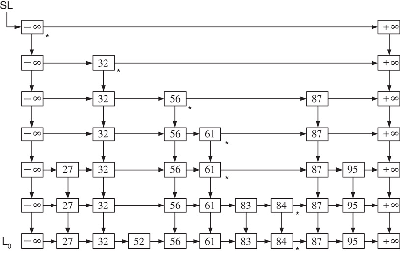
Figure 14.1A Skip List. The starred nodes are marked by Mark(86,SL).

How do we arrive at a leveling for a given set? We may construct S_i+1 from S_i in a systematic, deterministic way. While this may not pose any problem for a static search problem, it will be extremely cumbersome to implement the dynamic dictionary operations. This is where randomness is helpful. To get S_i+1 from S_i, we do the following. For each element k of S_i toss a coin and include k in S_i+1 iff we get success in the coin toss. If the coin is p-biased, we expect |S_i+1| to be roughly equal to p|S_i|. Starting from S, we may repeatedly obtain sets corresponding to successive levels. Since the coin tosses are independent, there is another useful, and equivalent way to look at our construction. For each key k in S, keep tossing a coin until we get a failure. Let h be the number of successes before the first failure. Then, we include k in h further levels treating S = S0 as the base level. In other words, we include k in the sets S1, S2, …, S_h. This suggests us to define a random variable Z_i for each key k_i ∈ S0 to be the number of times we toss a p-biased coin before we obtain a failure. Since Z_i denotes the number of additional copies of k_i in the skip list, the value maximum{Z_i:1 ≤ i ≤ n} defines the highest nonempty level. Hence, we have,

$\begin{aligned} r & = 1 + m a x i m u m {Z_{i} : 1 \leq i \leq n} \end{aligned}$ $\begin{aligned} r & = 1 + m a x i m u m {Z_{i} : 1 \leq i \leq n} \end{aligned}$	(14.8)

$\begin{aligned} ∣ S L ∣ & = n + Z_{1} + Z_{2} + \dots + Z_{n} + 2 r + 2 \end{aligned}$ $\begin{aligned} ∣ S L ∣ & = n + Z_{1} + Z_{2} + \dots + Z_{n} + 2 r + 2 \end{aligned}$	(14.9)

where r is the number of levels and |SL| is the number of boxes or the space complexity measure of the Skip List. In the expression for |SL| we have added n to count the keys in the base level and 2r + 2 counts the sentinel boxes containing + ∞ and − ∞ in each level.

14.4Structural Properties of Skip Lists

14.4.1Number of Levels in Skip List

Recall that r = 1 + max_i{Z_i}. Notice that Z_i ≥ k iff the coin tossed for k_i gets a run of at least k successes right from the beginning and this happens with probability pk. Since r ≥ k iff at least one of Z_i ≥ k − 1 , we easily get the following fact from Boole’s inequality

P r (r \geq k) \leq n p^{k - 1}

$P r (r \geq k) \leq n p^{k - 1}$

Choosing k = 4 log_1/p n + 1, we immediately obtain a high confidence bound for the number of levels. In fact,

$\begin{aligned} P r (r \geq 4 \log n + 1) & \leq n n^{- 4} \\ = \frac{1}{n^{3}} \end{aligned}$ $\begin{aligned} P r (r \geq 4 \log n + 1) & \leq n n^{- 4} \\ = \frac{1}{n^{3}} \end{aligned}$	(14.10)

We obtain an estimation for the expected value of r, using the formula stated in theorem (14.3) as follows:

\begin{array}{l} E (r) & = \sum_{i = 1}^{\infty} P r (r \geq i) \\ = \sum_{i = 1}^{4 \log n} P r (r \geq i) + \sum_{i > 4 \log n} P r (r \geq i) \\ \leq \sum_{i = 1}^{4 \log n} 1 + \sum_{i > 4 \log n}^{\infty} n p^{i - 1} \\ = 4 \log n + n p^{4 \log n} (1 + p + p^{2} + \dots) \\ = 4 \log n + n \cdot \frac{1}{n^{4}} \cdot (1 - p)^{- 1} if base of the \log is 1 / p \\ \leq 4 \log n + 1 for sufficiently large n \end{array}

$\begin{array}{l} E (r) & = \sum_{i = 1}^{\infty} P r (r \geq i) \\ = \sum_{i = 1}^{4 \log n} P r (r \geq i) + \sum_{i > 4 \log n} P r (r \geq i) \\ \leq \sum_{i = 1}^{4 \log n} 1 + \sum_{i > 4 \log n}^{\infty} n p^{i - 1} \\ = 4 \log n + n p^{4 \log n} (1 + p + p^{2} + \dots) \\ = 4 \log n + n \cdot \frac{1}{n^{4}} \cdot (1 - p)^{- 1} if base of the \log is 1 / p \\ \leq 4 \log n + 1 for sufficiently large n \end{array}$

Thus E(r) = O(log n)

Hence,

Theorem 14.11

The expected number of levels in a skip list of n elements is O(log n). In fact, the number is O(log n) with high probability.

14.4.2Space Complexity

Recall that the space complexity, |SL| is given by

∣ S L ∣= Z_{1} + Z_{2} + \dots + Z_{n} + n + 2 r + 2.

$∣ S L ∣= Z_{1} + Z_{2} + \dots + Z_{n} + n + 2 r + 2.$

As we know that r = O(log n) with high probability, let us focus on the sum

Z = Z_{1} + Z_{2} + \dots + Z_{n} .

$Z = Z_{1} + Z_{2} + \dots + Z_{n} .$

Since Z_i is a geometric random variable with parameter p, Z is a negative binomial random variable by theorem 14.6.

Thus $E (Z) = \frac{n}{p} = O (n)$ $E (Z) = \frac{n}{p} = O (n)$ .

We can in fact show that Z is O(n) with very high probability.

Now, from theorem (14.10) Pr(Z > 4n) = Pr(X < n) where X is a binomial distribution with parameters 4n and p. We now assume that p = 1/2 just for the sake of simplicity in arithmetic.

In the first Chernoff bound mentioned in theorem (14.9), replacing n, μ and k respectively with 4n, 2n and n, we obtain,

\begin{aligned} P r (X < n) & \leq {(\frac{2 n}{n})}^{n} {(\frac{2 n}{3 n})}^{3 n} \\ = {(2 \cdot \frac{2^{3}}{3^{3}})}^{n} \\ = {(\frac{16}{27})}^{n} \\ = {(\frac{27}{16})}^{- n} \end{aligned}

$\begin{aligned} P r (X < n) & \leq {(\frac{2 n}{n})}^{n} {(\frac{2 n}{3 n})}^{3 n} \\ = {(2 \cdot \frac{2^{3}}{3^{3}})}^{n} \\ = {(\frac{16}{27})}^{n} \\ = {(\frac{27}{16})}^{- n} \end{aligned}$

This implies that 4n is in fact a very high confidence bound for Z. Since |SL| = Z + n + 2r + 2, we easily conclude that

Theorem 14.12

The space complexity of a skip list for a set of size n is O(n) with very high probability.

14.5Dictionary Operations

We shall use a simple procedure called Mark in all the dictionary operations. The procedure Mark takes an arbitrary value x as input and marks in each level the box containing the largest key that is less than x. This property implies that insertion, deletion or search should all be done next to the marked boxes. Let M_i(x) denote the box in the ith level that is marked by the procedure call Mark(x, SL). Recall the convention used in the linked structure that name of a box in a linked list is nothing but a pointer to that box. The keys in the marked boxes M_i(x) satisfy the following condition :

$k e y [M_{i} (x)] < x \leq k e y [H n e x t [M_{i} (x)]] for all 0 \leq i \leq r .$ $k e y [M_{i} (x)] < x \leq k e y [H n e x t [M_{i} (x)]] for all 0 \leq i \leq r .$	(14.11)

The procedure Mark begins its computation at the box containing − ∞ in level r. At any current level, we traverse along the level using horizontal pointers until we find that the next box is containing a key larger or equal to x. When this happens, we mark the current box and use the descent pointer to reach the next lower level and work at this level in the same way. The procedure stops after marking a box in level 0. See Figure 14.1 for the nodes marked by the call Mark(86,SL).

 Algorithm Mark(x,SL)
 -- x is an arbitrary value.
 -- r is the number of levels in the skip list SL.
 1. Temp = SL.
 2. For i = r down to 0 do
    While (key[Hnext[Temp]] < x)
        Temp = Hnext[Temp];
    Mark the box pointed by Temp;
    Temp = Dnext[Temp];
 3. End.

We shall now outline how to use marked nodes for Dictionary operations. Let M0(x) be the box in level 0 marked by Mark(x). It is clear that the box next to M0(x) will have x iff x ∈ S. Hence our algorithm for Search is rather straight forward.

To insert an item in the Skip List, we begin by marking the Skip List with respect to the value x to be inserted. We assume that x is not already in the Skip List. Once the marking is done, inserting x is very easy. Obviously x is to be inserted next to the marked boxes. But in how many levels we insert x? We determine the number of levels by tossing a coin on behalf of x until we get a failure. If we get h successes, we would want x to be inserted in all levels from 0 to h. If h ≥ r, we simply insert x at all the existing levels and create a new level consisting of only − ∞ and + ∞ that corresponds to the empty set. The insertion will be done starting from the base level. However, the marked boxes are identified starting from the highest level. This means, the Insert procedure needs the marked boxes in the reverse order of its generation. An obvious strategy is to push the marked boxes in a stack as and when they are marked in the Mark procedure. We may pop from the stack as many marked boxes as needed for insertion and then insert x next to each of the popped boxes.

The deletion is even simpler. To delete a key x from S, simply mark the Skip List with respect to x. Note that if x is in L_i, then it will be found next to the marked box in L_i. Hence, we can use the horizontal pointers in the marked boxes to delete x from each level where x is present. If the deletion creates one or more empty levels, we ignore all of them and retain only one level corresponding to the empty set. In other words, the number of levels in the Skip List is reduced in this case. In fact, we may delete an item “on the fly” during the execution of the Mark procedure itself. As the details are simple we omit pseudo codes for these operations.

14.6Analysis of Dictionary Operations

It is easy to see that the cost of Search, Insert and Delete operations are dominated by the cost of Mark procedure. Hence we shall analyze only the Mark procedure. The Mark procedure starts at the ‘r’th level and proceeds like a downward walk on a staircase and ends at level 0. The complexity of Mark procedure is clearly proportional to the number of edges it traversed. It is advantageous to view the same path as if it is built from level 0 to level r. In other words, we analyze the building of the path in a direction opposite to the direction in which it is actually built by the procedure. Such an analysis is known as backward analysis.

Henceforth let P denote the path from level 0 to level r traversed by Mark(x) for the given fixed x. The path P will have several vertical edges and horizontal edges. (Note that at every box either P moves vertically above or moves horizontally to the left). Clearly, P has r vertical edges. To estimate number of horizontal edges, we need the following lemmas.

Lemma 14.6

Let the box b containing k at level i be marked by Mark(x). Let a box w containing k be present at level i + 1. Then, w is also marked.

Proof. Since b is marked, from Equation 14.11, we get that there is no value between k and x in level i. This fact holds good for L_i+1 too because S_i+1 ⊆ S_i. Hence the lemma.■

Lemma 14.7

Let the box b containing k at level i be marked by Mark(x). Let k ∉ L_i+1. Let u be the first box to the left of b in L_i having a “vertical neighbor” w. Then w is marked.

Proof. Let w.key = u.key = y. Since b is marked, k satisfies condition (14.11). Since u is the first node in the left of b having a vertical neighbor, none of the keys with values in between y and x will be in L_i+1. Also, k ∉ L_i+1 according to our assumption in the lemma. Thus y is the element in L_i+1 that is just less than x. That is, y satisfies the condition (14.11) at level i + 1. Hence the w at level i + 1 will be marked.■

Lemmas (14.6 and 14.7) characterize the segment of P between two successive marked boxes. This allows us to give an incremental description of P in the following way.

P starts from the marked box at level 0. It proceeds vertically as far as possible (Lemma 14.6) and when it cannot proceed vertically it proceeds horizontally. At the “first” opportunity to move vertically, it does so (Lemma 14.7), and continues its vertical journey. Since for any box a vertical neighbor exists only with a probability p, we see that P proceeds from the current box vertically with probability p and horizontally with probability (1 − p).

Hence, the number of horizontal edges of P in level i is a geometric random variable, say, Y_i, with parameter (1 − p). Since the number of vertical edges in P is exactly r, we conclude,

Theorem 14.13

The number of edges traversed by Mark(x) for any fixed x is given by |P| = r + (Y0 + Y1 + Y2 + ··· + Y_{r − 1}) where Y_i is a geometric random variable with parameters 1 − p and r is the random variable denoting the number of levels in the Skip List.

Our next mission is to obtain a high confidence bound for the size of P. As we have already derived high confidence bound for r, let focus on the sum H_r = Y0 + Y1 + ··· + Y_r−1 for a while. Since r is a random variable H_r is not a deterministic sum of random variables but a random sum of random variables.

Hence we cannot directly apply theorem (14.6) and the bounds for negative binomial distributions.

Let X be the event of the random variable r taking a value less than or equal to 4 log n. Note that $P (\bar{X}) < \frac{1}{n^{3}}$ $P (\bar{X}) < \frac{1}{n^{3}}$ by (14.10).

From the law of total probability, Boole’s inequality and equation (14.10) we get,

\begin{aligned} P r (H_{r} > 16 \log n) & = P r ([H_{r} > 16 \log n] \cap X) + P r ([H_{r} > 16 \log n] \cap \bar{X}) \\ = P r ([H_{r} > 16 \log n] \cap r \leq 4 \log n) + P r ([H_{r} > 16 \log n] \cap \bar{X}) \\ \leq \sum_{k = 0}^{4 \log n} P r (H_{k} > 16 \log n) + P r (\bar{X}) \\ \leq (1 + 4 \log n) P r (H_{4 \log n} > 16 \log n) + \frac{1}{n^{3}} \end{aligned}

$\begin{aligned} P r (H_{r} > 16 \log n) & = P r ([H_{r} > 16 \log n] \cap X) + P r ([H_{r} > 16 \log n] \cap \bar{X}) \\ = P r ([H_{r} > 16 \log n] \cap r \leq 4 \log n) + P r ([H_{r} > 16 \log n] \cap \bar{X}) \\ \leq \sum_{k = 0}^{4 \log n} P r (H_{k} > 16 \log n) + P r (\bar{X}) \\ \leq (1 + 4 \log n) P r (H_{4 \log n} > 16 \log n) + \frac{1}{n^{3}} \end{aligned}$

Now Pr(H_{4 log n} > 16 log n) can be computed in a manner identical to the one we carried out in the space complexity analysis. Notice that H_{4 log n} is a deterministic sum of geometric random variables. Hence we can apply theorems (14.9) and (14.10) to derive a high confidence bound. Specifically, by theorem (14.10),

P r (H_{4 \log n} > 16 \log n) = P r (X < 4 \log n),

$P r (H_{4 \log n} > 16 \log n) = P r (X < 4 \log n),$

where X is a binomial random variable with parameters 16 log n and p. Choosing p = 1/2 allows us to set μ = 8 log n, k = 4 log n and replace n by 16 log n in the first inequality of theorem (14.9). Putting all these together we obtain,

\begin{aligned} P r (H_{4 \log n} > 16 \log n) & = P r (X < 4 \log n) \\ \leq {(\frac{8 \log n}{4 \log n})}^{4 \log n} {(\frac{8 \log n}{12 \log n})}^{12 \log n} \\ = {(2 \cdot \frac{2^{3}}{3^{3}})}^{4 \log n} \\ = {(\frac{16}{27})}^{4 \log n} \\ < {(\frac{1}{8})}^{\log n} \\ = \frac{1}{n^{3}} \end{aligned}

$\begin{aligned} P r (H_{4 \log n} > 16 \log n) & = P r (X < 4 \log n) \\ \leq {(\frac{8 \log n}{4 \log n})}^{4 \log n} {(\frac{8 \log n}{12 \log n})}^{12 \log n} \\ = {(2 \cdot \frac{2^{3}}{3^{3}})}^{4 \log n} \\ = {(\frac{16}{27})}^{4 \log n} \\ < {(\frac{1}{8})}^{\log n} \\ = \frac{1}{n^{3}} \end{aligned}$

Therefore

\begin{aligned} P r (H_{r} > 16 \log n) & < (1 + 4 \log n) (\frac{1}{n^{3}}) + \frac{1}{n^{3}} \\ < \frac{1}{n^{2}} i f n \geq 32 \end{aligned}

$\begin{aligned} P r (H_{r} > 16 \log n) & < (1 + 4 \log n) (\frac{1}{n^{3}}) + \frac{1}{n^{3}} \\ < \frac{1}{n^{2}} i f n \geq 32 \end{aligned}$

This completes the derivation of a high confidence bound for H_r. From this, we can easily obtain a bound for expected value of H_r. We use theorem (14.3) and write the expression for E(H_r) as

E (H_{r}) = \sum_{i = 1}^{16 \log n} P r (H_{r} \geq i) + \sum_{i > 16 \log n} P r (H_{r} \geq i) .

$E (H_{r}) = \sum_{i = 1}^{16 \log n} P r (H_{r} \geq i) + \sum_{i > 16 \log n} P r (H_{r} \geq i) .$

The first sum is bounded above by 16 log n as each probability value is less than 1 and by the high confidence bound that we have established just now, we see that the second sum is dominated by $\sum_{i = 1}^{\infty} 1 / i^{2}$ $\sum_{i = 1}^{\infty} 1 / i^{2}$ which is a constant. Thus we obtain,

E (H_{r}) \leq 16 \log n + c = O (\log n) .

$E (H_{r}) \leq 16 \log n + c = O (\log n) .$

Since P = r + H_r we easily get that E(|P|) = O(log n) and |P| = O(log n) with probability greater than $1 - O (\frac{1}{n^{2}})$ $1 - O (\frac{1}{n^{2}})$ . Observe that we have analyzed Mark(x) for a given fixed x. To show that the high confidence bound for any x, we need to proceed little further. Note that there are only n + 1 distinct paths possible with respect to the set { − ∞ = k0, k1, …, k_n, k_{n + 1} = + ∞}, each corresponding to the x lying in the internal [k_i, k_i+1), i = 0, 1, …, n.

Therefore, for any x, Mark(x) walks along a path P satisfying E(|P|) = O(log n) and |P| = O(log n) with probability greater than $1 - O (\frac{1}{n})$ $1 - O (\frac{1}{n})$ .

Summarizing,

Theorem 14.14

The Dictionary operations Insert, Delete, and Search take O(log n) expected time when implemented using Skip Lists. Moreover, the running time for Dictionary operations in a Skip List is O(log n) with high probability.

14.7Randomized Binary Search Trees

A Binary Search Tree (BST) for a set S of keys is a binary tree satisfying the following properties.

a.Each node has exactly one key of S. We use the notation v.key to denote the key stored at node v.

b.For all node v and for all nodes u in the left subtree of v and for all nodes w in the right subtree of v, the keys stored in them satisfy the so called search tree property:

u . k e y < v . k e y < w . k e y

$u . k e y < v . k e y < w . k e y$

The complexity of the dictionary operations are bounded by the height of the binary search tree. Hence, ways and means were explored for controlling the height of the tree during the course of execution. Several clever balancing schemes were discovered with varying degrees of complexities. In general, the implementation of balancing schemes are tedious and we may have to perform a number of rotations which are complicated operations. Another line of research explored the potential of possible randomness in the input data. The idea was to completely avoid balancing schemes and hope to have “short” trees due to randomness in input. When only random insertion are done, we obtain so called Randomly Built Binary Tree (RBBT). RBBTs have been shown to have O(log n) expected height.

What is the meaning of random insertion? Suppose we have already inserted the values a1, a2, a3, …, a_k−1. These values, when considered in sorted order, define k intervals on the real line and the new value to be inserted, say x, is equally likely to be in any of the k intervals.

The first drawback of RBBT is that this assumption may not be valid in practice and when this assumption is not satisfied, the resulting tree structure could be highly skewed and the complexity of search as well as insertion could be as high as O(n). The second major drawback is when deletion is also done on these structures, there is a tremendous degradation in the performance. There is no theoretical results available and extensive empirical studies show that the height of an RBBT could grow to $O (\sqrt{n})$ $O (\sqrt{n})$ when we have arbitrary mix of insertion and deletion, even if the randomness assumption is satisfied for inserting elements. Thus, we did not have a satisfactory solution for nearly three decades.

In short, the randomness was not preserved by the deletion operation and randomness preserving binary tree structures for the dictionary operations was one of the outstanding open problems, until an elegant affirmative answer is provided by Martinez and Roura in their landmark paper [4].

In this section, we shall briefly discuss about structure proposed by Martinez and Roura.

Definition 14.15: (Randomized Binary Search Trees)

Let T be a binary search tree of size n. If n = 0, then T = NULL and it is a random binary search tree. If n > 0, T is a random binary search tree iff both its left subtree L and right subtree R are independent random binary search trees and

Pr {S i z e (L) = i | S i z e (T) = n} = \frac{1}{n}, 0 \leq i \leq n .

$Pr {S i z e (L) = i | S i z e (T) = n} = \frac{1}{n}, 0 \leq i \leq n .$

The above definition implies that every key has the same probability of $\frac{1}{n}$ $\frac{1}{n}$ for becoming the root of the tree. It is easy to prove that the expected height of a RBST with n nodes is O(log n). The RBSTs possess a number of interesting structural properties and the classic book by Mahmoud [5] discusses them in detail. In view of the above fact, it is enough if we prove that when insert or delete operation is performed on a RBST, the resulting tree is also an RBST.

14.7.1Insertion in RBST

When a key x is inserted in a tree T of size n, we obtain a tree T′ of size n + 1. For T′, as we observed earlier, x should be in the root with probability $\frac{1}{n + 1}$ $\frac{1}{n + 1}$ . This is our starting point.

 Algorithm Insert(x, T)
 - L is the left subtree of the root
 - R is the right subtree of the root
 1. n = size(T);
 2. r = random(0, n);
 3. If (r = n) then
      Insert_at_root(x, T);
 4. If (x < key at root of T) then
      Insert(x, L);
    Else
      Insert(x, R);

To insert x as a root of the resulting tree, we first split the current tree into two trees labeled T_< and T_>, where T_< contains all the keys in T that are smaller than x and T_> contains all the keys in T that are larger than x. The output tree T′ is constructed by placing x at the root and attaching T_< as its left subtree and T_> as its right subtree. The algorithm for splitting a tree T into T_< and T_> with respect to a value x is similar to the partitioning algorithm done in quicksort. Specifically, the algorithm split(x,T) works as follows. If T is empty, nothing needs to be done; both T_< and T_> are empty. When T is non-empty we compare x with Root(T).key. If x < Root(T).key, then root of T as well as the right subtree of T belong to T_>. To compute T_< and the remaining part of T_> we recursively call split(x, L), where L is the left subtree for the root of T. If x > Root(T).key, T_< is built first and recursion proceeds with split(x, R). The details are left as easy exercise.

We shall first prove that T_< and T_> are independent Random Binary Search Trees. Formally,

Theorem 14.15

Let T_< and T_> be the BSTs produced by split(x, T). If T is a random BST containing the set of keys S, then T_< and T_> are RBBTs containing the keys S< = {y ∈ S|y < x} and S> = {y ∈ S|y > x}, respectively.

Proof. Let size(T) = n > 0, x > Root(T).key, we will show that for any z ∈ S<, the probability that z is the root of T_< is 1/m where m = size(T_<). In fact,

\begin{aligned} Pr (z is root of T_{<} ∣ root of T is less than x) \\ = \frac{Pr (z is root of T_{<} and root of T is less than x)}{Pr(root of T is less than x)} \\ = \frac{1 / n}{m / n} = \frac{1}{m} . \end{aligned}

$\begin{aligned} Pr (z is root of T_{<} ∣ root of T is less than x) \\ = \frac{Pr (z is root of T_{<} and root of T is less than x)}{Pr(root of T is less than x)} \\ = \frac{1 / n}{m / n} = \frac{1}{m} . \end{aligned}$

The independence of T_< and T_> follows from the independence of L and R of T and by induction. ■

We are now ready to prove that randomness is preserved by insertion. Specifically,

Theorem 14.16

Let T be a RBST for the set of keys S and x ∉ S, and assume that insert(s, T) produces a tree, say T′ for S ∪ {x}. Then, T′ is a RBST.

Proof. A key y ∈ S will be at the root of T′ iff

1.y is at root of T.

2.x is not inserted at the root of T′

As (1) and (2) are independent events with probability $\frac{1}{n}$ $\frac{1}{n}$ and $\frac{n}{n + 1}$ $\frac{n}{n + 1}$ , respectively, it follows that Prob(y is at root of T′) $= \frac{1}{n} \cdot \frac{n}{n + 1} = \frac{1}{n + 1}$ $= \frac{1}{n} \cdot \frac{n}{n + 1} = \frac{1}{n + 1}$ . The key x can be at the root of T′ only when insert(x, T) invokes insert-at-root(x, T) and this happens with probability $\frac{1}{n + 1}$ $\frac{1}{n + 1}$ . Thus, any key in S ∪ {x} has the probability of $\frac{1}{n + 1}$ $\frac{1}{n + 1}$ for becoming the root of T′. The independence of left and right subtrees of T′ follows from independence of left and right subtrees of T, induction, and the previous theorem. ■

14.7.2Deletion in RBST

Suppose x ∈ T and let T_x denote the subtree of T rooted at x. Assume that L and R are the left and right subtrees of T_x. To delete x, we build a new BST T_x = Join(L, R) containing the keys in L and R and replace T_x by T_x. Since pseudocode for deletion is easy to write, we omit the details.

We shall take a closer look at the details of the Join routine. We need couple of more notations to describe the procedure Join. Let L_l and L_r denote the left and right subtrees of L and R_l and R_r denote the left and right subtrees of R, respectively. Let a denote the root of L and b denote the root of R. We select either a or b to serve as the root of T_x with appropriate probabilities. Specifically, the probability for a becoming the root of T_x is $\frac{m}{m + n}$ $\frac{m}{m + n}$ and for b it is $\frac{n}{n + m}$ $\frac{n}{n + m}$ where m = size(L) and n = size(R).

If a is chosen as the root, the its left subtree L_l is not modified while its right subtree L_r is replaced with Join(L_r, R). If b is chosen as the root, then its right subtree R_r is left intact but its left subtree R_l is replaced with Join(L, R_l). The join of an empty tree with another tree T is T it self and this is the condition used to terminate the recursion.

 Algorithm Join(L,R)
 -- L and R are RBSTs with roots a and b and size m and n respectively.
 -- All keys in L are strictly smaller than all keys in R.
 -- $L_l$ and $L_r$ respectively denote the left and right subtree of L.
 -- $R_l$ and $R_r$ are similarly defined for R.

 1. If ( L is NULL) return R.
 2. If ( R is NULL) return L.
 3. Generate a random integer i in the range [0, n+m-1].
 4. If ( i < m ) {* the probability for this event is m/(n+m).*}
      L_r = Join(L_l,R);
      return L;
    else   {* the probability for this event is n/(n+m).*}
      R_l = Join(L,R_l);
      return R;

It remains to show that Join of two RBSTs produces RBST and deletion preserves randomness in RBST.

Theorem 14.17

The Algorithm Join(L,R) produces a RBST under the conditions stated in the algorithm.

Proof. We show that any key has the probability of 1/(n + m) for becoming the root of the tree output by Join(L,R). Let x be a key in L. Note that x will be at the root of Join(L,R) iff

•x was at the root of L before the Join operation, and,

•The root of L is selected to serve as the root of the output tree during the Join operation.

The probability for the first event is 1/m and the second event occurs with probability m/(n + m). As these events are independent, it follows that the probability of x at the root of the output tree is $\frac{1}{m} \cdot \frac{m}{n + m} = \frac{1}{n + m}$ $\frac{1}{m} \cdot \frac{m}{n + m} = \frac{1}{n + m}$ . A similar reasoning holds good for the keys in R. ■

Finally,

Theorem 14.18

If T is a RBST for a set K of keys, then Delete(x,T) outputs a RBST for K − {x}.

Proof. We sketch only the chance counting argument. The independence of the subtrees follows from the properties of Join operation and induction. Let T′ = Delete(x, T). Assume that x ∈ K and size of K is n. We have to prove that for any y ∈ K, y ≠ x, the probability for y in root of T′ is 1/(n − 1). Now, y will be at the root of T′ iff either x was at the root of T and its deletion from T brought y to the root of T′ or y was at the root of T(so that deletion of x from T did not dislocate y). The former happens with a probability $\frac{1}{n} \cdot \frac{1}{n - 1}$ $\frac{1}{n} \cdot \frac{1}{n - 1}$ and the probability of the later is $\frac{1}{n}$ $\frac{1}{n}$ . As these events are independent, we add the probabilities to obtain the desired result.■

14.8Bibliographic Remarks

In this chapter we have discussed two randomized data structures for Dictionary ADT. Skip Lists are introduced by Pugh in 1990 [3]. A large number of implementations of this structure by a number of people available in the literature, including the one by the inventor himself. Sedgewick gives an account of the comparison of the performances of Skip Lists with the performances of other balanced tree structures [6]. See [7] for a discussion on the implementation of other typical operations such as merge. Pugh argues how Skip Lists are more efficient in practice than balanced trees with respect to Dictionary operations as well as several other operations. Pugh has further explored the possibilities of performing concurrent operations on Skip Lists in Reference [8]. For a more elaborate and deeper analysis of Skip Lists, refer the PhD thesis of Papadakis [9]. In his thesis, he has introduced deterministic skip lists and compared and contrasted the same with a number of other implementations of Dictionaries. Sandeep Sen [10] provides a crisp analysis of the structural properties of Skip Lists. Our analysis presented in this chapter is somewhat simpler than Sen’s analysis and our bounds are derived based on different tail estimates of the random variables involved.

The randomized binary search trees are introduced by Martinez and Roura in their classic paper [4] which contains many more details than discussed in this chapter. In fact, we would rate this paper as one of the best written papers in data structures. Seidel and Aragon have proposed a structure called probabilistic priority queues [11] and it has a comparable performance. However, the randomness in their structure is achieved through randomly generated real numbers (called priorities) while the randomness in Martinez and Roura’s structure is inherent in the tree itself. Besides this being simpler and more elegant, it solves one of the outstanding open problems in the area of search trees.

References

1.P. Raghavan and R. Motwani, Randomized Algorithms, Cambridge University Press, USA, 1995.

2.T. Hagerup and C. Rub, A guided tour of Chernoff bounds, Information Processing Letters, 33:305–308, 1990.

3.W. Pugh, Skip Lists: A probabilistic alternative to balanced trees, Communications of the ACM, 33:668–676, 1990.

4.C. Martinez and S. Roura, Randomized binary search trees, Journal of the ACM, 45:288–323, 1998.

5.H. M. Mahmoud, Evolution of Random Search Trees, Wiley Interscience, USA, 1992.

6.R. Sedgewick, Algorithms, Third edition, Addison-Wesley, USA, 1998.

7.W. Pugh, A Skip List cook book, Technical report, CS-TR-2286.1, University of Maryland, USA, 1990.

8.W. Pugh, Concurrent maintenance of Skip Lists, Technical report, CS-TR-2222, University of Maryland, USA, 1990.

9.Th. Papadakis, Skip List and probabilistic analysis of algorithms, PhD Thesis, University of Waterloo, Canada, 1993. (Available as Technical Report CS-93-28).

10.S. Sen, Some observations on Skip Lists, Information Processing Letters, 39:173–176, 1991.

11.R. Seidel and C. Aragon, Randomized Search Trees, Algorithmica, 16:464–497, 1996.

^* This chapter has been reprinted from first edition of this Handbook, without any content updates.

..................Content has been hidden....................

You can't read the all page of ebook, please click here login for view all page.

Table of Contents for 14. Randomized Dictionary Structures

Create new playlist

Sign In

Sign Up

Table of Contents for
14. Randomized Dictionary Structures