
Narsingh Deo
University of Central Florida
4.3Connectivity, Distance, and Spanning Trees
Depth-First Search•Breadth-First Search
4.5Simple Applications of DFS and BFS
Depth-First Search on a Digraph•Topological Sorting
Kruskal’s MST Algorithm•Prim’s MST Algorithm•Boruvka’s MST Algorithm•Constrained MST
Single-Source Shortest Paths, Nonnegative Weights•Single-Source Shortest Paths, Arbitrary Weights•All-Pairs Shortest Paths
4.8Eulerian and Hamiltonian Graphs
Trees, as data structures, are somewhat limited because they can only represent relations of a hierarchical nature, such as that of parent and child. A generalization of a tree so that a binary relation is allowed between any pair of elements would constitute a graph—formally defined as follows:
A graph G = (V, E) consists of a finite set of vertices V = {υ1, υ2,…, υn} and a finite set E of edges E = {e1, e2,…, em} (see Figure 4.1). To each edge e there corresponds a pair of vertices (u, υ) which e is said to be incident on. While drawing a graph we represent each vertex by a dot and each edge by a line segment joining its two end vertices. A graph is said to be a directed graph (or digraph for short) (see Figure 4.2) if the vertex pair (u, υ) associated with each edge e (also called arc) is an ordered pair. Edge e is then said to be directed from vertex u to vertex υ, and the direction is shown by an arrowhead on the edge. A graph is undirected if the end vertices of all the edges are unordered (i.e., edges have no direction). Throughout this chapter we use the letters n and m to denote the number of vertices |V| and number of edges |E| respectively, in a graph. A vertex is often referred to as a node (a term more popular in applied fields).

Figure 4.1Undirected graph with 5 vertices and 6 edges.

Figure 4.2Digraph with 6 vertices and 11 edges.
Two or more edges having the same pair of end vertices are called parallel edges or multi edges, and a graph with multi edges is sometimes referred to as a multigraph. An edge whose two end vertices are the same is called a self-loop (or just loop). A graph in which neither parallel edges nor self loops are allowed is often called a simple graph. If both self-loops and parallel edges are allowed we have a general graph (also referred to as pseudograph). Graphs in Figures 4.1 and 4.2 are both simple but the graph in Figure 4.3 is pseudograph. If the graph is simple we can refer to each edge by its end vertices. The number of edges incident on a vertex v, with self-loops counted twice, is called the degree, deg(v), of vertex v. In directed graphs a vertex has in-degree (number of edges going into it) and out-degree (number of edges going out of it).

Figure 4.3A pseudograph of 6 vertices and 10 edges.
In a digraph if there is a directed edge (x, y) from x to y, vertex y is called a successor of x and vertex x is called a predecessor of y. In case of an undirected graph two vertices are said to be adjacent or neighbors if there is an edge between them.
A weighted graph is a (directed or undirected) graph in which a real number is assigned to each edge. This number is referred to as the weight of that edge. Weighted directed graphs are often referred to as networks. In a practical network this number (weight) may represent the driving distance, the construction cost, the transit time, the reliability, the transition probability, the carrying capacity, or any other such attribute of the edge [1–4].
Graphs are the most general and versatile data structures. Graphs have been used to model and solve a large variety of problems in the discrete domain. In their modeling and problem solving ability graphs are to the discrete world what differential equations are to the world of the continuum.
For a given graph a number of different representations are possible. The ease of implementation, as well as the efficiency of a graph algorithm depends on the proper choice of the graph representation. The two most commonly used data structures for representing a graph (directed or undirected) are adjacency lists and adjacency matrix. In this section we discuss these and other data structures used in representing graphs.
Adjacency lists: The adjacency lists representation of a graph G consists of an array Adj of n linked lists, one for each vertex in G, such that Adj[υ] for vertex υ consists of all vertices adjacent to υ. This list is often implemented as a linked list. (Sometimes it is also represented as a table, in which case it is called the star representation [3].)
Adjacency Matrix: The adjacency matrix of a graph G = (V, E) is an n × n matrix A = [aij] in which aij = 1 if there is an edge from vertex i to vertex j in G; otherwise aij = 0. Note that in an adjacency matrix a self-loop can be represented by making the corresponding diagonal entry 1. Parallel edges could be represented by allowing an entry to be greater than 1, but doing so is uncommon, since it is usually convenient to represent each element in the matrix by a single bit. The adjacency lists and adjacency matrix of an undirected graph are shown in Figure 4.4, and the corresponding two representations for a digraph are shown in Figure 4.5.
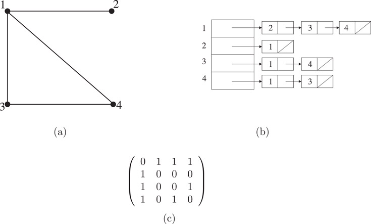
Figure 4.4An undirected graph (a) with four vertices and four edges; (b) its adjacency lists representation, and (c) its adjacency matrix representation.

Figure 4.5Two representations: (a) A digraph with five vertices and eight edges; (b) its adjacency lists representation, and (c) its adjacency matrix representation.
Clearly the memory required to store a graph of n vertices in the form of adjacency matrix is O(n2), whereas for storing it in the form of its adjacency lists is O(m + n). In general if the graph is sparse, adjacency lists are used but if the graph is dense, adjacency matrix is preferred. The nature of graph processing is an important factor in selecting the data structure.
There are other less frequently used data structures for representing graphs, such as forward or backward star, the edge-list, and vertex-edge incidence matrix [1–5].
4.2.1Weighted Graph Representation
Both adjacency lists and adjacency matrix can be adapted to take into account the weights associated with each edge in the graph. In the former case an additional field is added in the linked list to include the weight of the edge; and in the latter case the graph is represented by a weight matrix in which the (i, j)th entry is the weight of edge (i, j) in the weighted graph. These two representations for a weighted graph are shown in Figure 4.6. The boxed numbers next to the edges in Figure 4.6a are the weights of the corresponding edges.
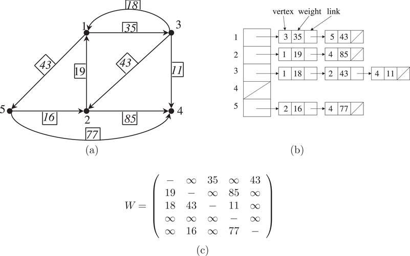
Figure 4.6Two representations: (a) A weighted digraph with five vertices and nine edges; (b) its adjacency lists, and (c) its weight matrix.
It should be noted that in a weight matrix, W, of a weighted graph, G, if there is no edge (i, j) in G, the corresponding element wij is usually set to ∞ (in practice, some very large number). The diagonal entries are usually set to ∞ (or to some other value depending on the application and algorithm). It is easy to see that the weight matrix of an undirected graph (like the adjacency matrix) is symmetric.
4.3Connectivity, Distance, and Spanning Trees
Just as two vertices x and y in a graph are said to be adjacent if there is an edge joining them, two edges are said to be adjacent if they share (i.e., are incident on) a common vertex. A simple path, or path for short, is a sequence of adjacent edges (υ1, υ2), (υ2, υ3), …, (υk − 2, υk − 1), (υk − 1, υk), sometimes written (υ1, υ2,…, υk), in which all the vertices υ1, υ2,…, υk are distinct except possibly υ1 = υk. In a digraph this path is said to be directed from υ1 to υk; in an undirected graph this path is said to be between υ1 and υk. The number of edges in a path, in this case, k − 1, is called the length of the path. In Figure 4.3 sequence (υ6, υ4), (υ4, υ1), (υ1, υ2) = (υ6, υ4, υ1, υ2) is a path of length 3 between υ6 and υ2. In the digraph in Figure 4.6 sequence (3, 1), (1, 5), (5, 2), (2, 4) = (3, 1, 5, 2, 4) is a directed path of length 4 from vertex 3 to vertex 4. A cycle or circuit is a path in which the first and the last vertices are the same. In Figure 4.3 (υ3, υ6, υ4, υ1, υ3) is a cycle of length 4. In Figure 4.6 (3, 2, 1, 3) is a cycle of length 3. A graph that contains no cycle is called acyclic.
A subgraph of a graph G = (V, E) is a graph whose vertices and edges are in G. A subgraph g of G is said to be induced by a subset of vertices S ⊆ V if g results when the vertices in V − S and all the edges incident on them are removed from G. For example, in Figure 4.3, the subgraph induced by {υ1, υ3, υ4} would consists of these three vertices and four edges {e3, e5, e6, e7}.
An undirected graph G is said to be connected if there is at least one path between every pair of vertices υi and υj in G. Graph G is said to be disconnected if it has at least one pair of distinct vertices u and v such that there is no path between u and v. Two vertices x and y in an undirected graph G = (V, E) are said to be connected if there exists a path between x and y. This relation of being connected is an equivalence relation on the vertex set V, and therefore it partitions the vertices of G into equivalence classes. Each equivalence class of vertices induces a subgraph of G. These subgraphs are called connected components of G. In other words, a connected component is a maximal connected subgraph of G. A connected graph consists of just one component, whereas a disconnected graph consists of several (connected) components. Each of the graphs in Figures 4.1, 4.3, and 4.4 is connected. But the graph given in Figure 4.7 is disconnected, consisting of four components.

Figure 4.7A disconnected graph of 10 vertices, 8 edges, and 4 components.
Notice that a component may consist of just one vertex such as j in Figure 4.7 with no edges. Such a component (subgraph or graph) is called an isolated vertex. Equivalently, a vertex with zero degree is called an isolated vertex. Likewise, a graph (subgraph or component) may consist of just one edge, such as edge (i, d) in Figure 4.7.
One of the simplest and often the most important and useful questions about a given graph G is: Is G connected? And if G is not connected what are its connected components? This question will be taken up in the next section, and an algorithm for determining the connected components will be provided; but first a few more concepts and definitions.
Connectivity in a directed graph G is more involved. A digraph is said to be connected if the undirected graph obtained by ignoring the edge directions in G is connected. A directed graph is said to be strongly connected if for every pair of vertices υi and υj there exists at least one directed path from υi to υj and at least one from υj to υi. A digraph which is connected but not strongly connected is called weakly connected. A disconnected digraph (like a disconnected undirected graph) consists of connected components; and a weakly-connected digraph consists of strongly-connected components. For example, the connected digraph in Figure 4.5 consists of four strongly-connected components—induced by each of the following subsets of vertices {1, 2},{3},{4}, and {5}.
Another important question is that of distance from one vertex to another. The distance from vertex a to b is the length of the shortest path (i.e., a path of the smallest length) from a to b, if such a path exists. If no path from a to b exists, the distance is undefined and is often set to ∞. Thus, the distance from a vertex to itself is 0; and the distance from a vertex to an adjacent vertex is 1. In an undirected graph distance from a to b equals the distance from b to a, that is, it is symmetric. It is also not difficult to see that the distances in a connected undirected graph (or a strongly connected digraph) satisfy the triangle inequality. In a connected, undirected (unweighted) graph G, the maximum distance between any pair of vertices is called the diameter of G.
A connected, undirected, acyclic (without cycles) graph is called a tree, and a set of trees is called a forest. We have already seen rooted trees and forests of rooted trees in the preceding chapter, but the unrooted trees and forests discussed in this chapter are graphs of a very special kind that play an important role in many applications.
In a connected undirected graph G there is at least one path between every pair of vertices and the absence of a cycle implies that there is at most one such path between any pair of vertices in G. Thus if G is a tree, there is exactly one path between every pair of vertices in G. The argument is easily reversed, and so an undirected graph G is a tree if and only if there is exactly one path between every pair of vertices in G. A tree with n vertices has exactly (n − 1) edges. Since (n − 1) edges are the fewest possible to connect n points, trees can be thought of as graphs that are minimally connected. That is, removing any edge from a tree would disconnect it by destroying the only path between at least one pair of vertices.
A spanning tree for a connected graph G is a subgraph of G which is a tree containing every vertex of G. If G is not connected, a set consisting of one spanning tree for each component is called a spanning forest of G. To construct a spanning tree (forest) of a given undirected graph G, we examine the edges of G one at a time and retain only those that do not not form a cycle with the edges already selected. Systematic ways of examining the edges of a graph will be discussed in the next section.
It is evident that for answering almost any nontrivial question about a given graph G we must examine every edge (and in the process every vertex) of G at least once. For example, before declaring a graph G to be disconnected we must have looked at every edge in G; for otherwise, it might happen that the one edge we had decided to ignore could have made the graph connected. The same can be said for questions of separability, planarity, and other properties [5,6].
There are two natural ways of scanning or searching the edges of a graph as we move from vertex to vertex: (i) once at a vertex v we scan all edges incident on v and then move to an adjacent vertex w, then from w we scan all edges incident on w. This process is continued till all the edges reachable from v are scanned. This method of fanning out from a given vertex v and visiting all vertices reachable from v in order of their distances from v (i.e., first visit all vertices at a distance one from v, then all vertices at distances two from v, and so on) is referred to as the breadth-first search (BFS) of the graph. (ii) An opposite approach would be, instead of scanning every edge incident on vertex v, we move to an adjacent vertex w (a vertex not visited before) as soon as possible, leaving v with possibly unexplored edges for the time being. In other words, we trace a path through the graph going on to a new vertex whenever possible. This method of traversing the graph is called the depth-first search (DFS). Breadth-first and depth-first searches are fundamental methods of graph traversal that form the basis of many graph algorithms [5–8]. The details of these two methods follow.
Depth-first search on an undirected graph G = (V, E) explores the graph as follows. When we are “visiting” a vertex v ∈ V, we follow one of the edges (v, w) incident on v. If the vertex w has been previously visited, we return to v and choose another edge. If the vertex w (at the other end of edge (v, w) from v) has not been previously visited, we visit it and apply the process recursively to w. If all the edges incident on v have been thus traversed, we go back along the edge (u, v) that had first led to the current vertex v and continue exploring the edges incident on u. We are finished when we try to back up from the vertex at which the exploration began.
Figure 4.8 illustrates how depth-first search examines an undirected graph G represented as an adjacency lists. We start with a vertex a. From a we traverse the first edge that we encounter, which is (a, b). Since b is a vertex never visited before, we stay at b and traverse the first untraversed edge encountered at b, which is (b, c). Now at vertex c, the first untraversed edge that we find is (c, a). We traverse (c, a) and find that a has been previously visited. So we return to c, marking the edge (c, a) in some way (as a dashed line in Figure 4.8c) to distinguish it from edges like (b, c), which lead to new vertices and shown as the thick lines. Back at vertex c, we look for another untraversed edge and traverse the first one that we encounter, which is (c, d). Once again, since d is a new vertex, we stay at d and look for an untraversed edge. And so on. The numbers next to the vertices in Figure 4.8c show the order in which they were visited; and the numbers next to the edges show the order in which they were traversed.

Figure 4.8A graph (a); its adjacency lists (b); and its depth-first traversal (c). The numbers are the order in which vertices were visited and edges traversed. Edges whose traversal led to new vertices are shown with thick lines, and edges that led to vertices that were already visited are shown with dashed lines.
Depth-first search performed on a connected undirected graph G = (V, E), partitions the edge set into two types: (i) Those that led to new vertices during the search constitute the branches of a spanning tree of G and (ii) the remaining edges in E are called back edges because their traversal led to an already visited vertex from which we backed down to the current vertex.
A recursive depth-first search algorithm is given in Figure 4.9. Initially, every vertex x is marked unvisited by setting num[x] to 0. Note that in the algorithm shown in Figure 4.9, only the tree edges are kept track of. The time complexity of the depth-first search algorithm is O(m + n), provided the input is in the form of an adjacency matrix.

Figure 4.9Algorithm for depth-first search on an undirected graph G.
In breadth-first search we start exploring from a specified vertex s and mark it “visited.” All other vertices of the given undirected graph G are marked as “unvisited” by setting num[] = 0. Then we visit all vertices adjacent to s (i.e., in the adjacency list of s). Next, we visit all unvisited vertices adjacent to the first vertex in the adjacency list of s. Unlike the depth-first search, in breadth-first search we explore (fan out) from vertices in order in which they themselves were visited. To implement this method of search, we maintain a queue (Q) of visited vertices. As we visit a new vertex for the first time, we place it in (i.e., at the back of) the queue. We take a vertex v from front of the queue and traverse all untraversed edges incident at v—adding to the list of tree edges those edges that lead to unvisited vertices from v ignoring the rest. Once a vertex v has been taken out of the queue, all the neighbors of v have been visited and v is completely explored.
Thus, during the execution of a breadth-first search we have three types of vertices: (i) unvisited, those that have never been in the queue; (ii) completely explored, those that have been in the queue but are not now in the queue; and (iii) visited but not completely explored, that is, those that are currently in the queue.
Since every vertex (reachable from the start vertex s) enters and exits the queue exactly once and every edge in the adjacency list of a vertex is traversed exactly once, the time complexity of the breadth-first search is O(n + m).
An algorithm for performing a breadth-first search on an undirected connected graph G from a specified vertex s is given in Figure 4.10. It produces a breadth-first tree in G rooted at vertex s. For example, the spanning tree produced by BFS conducted on the graph in Figure 4.8 starting at vertex a, is shown in Figure 4.11. The numbers next to the vertices show the order in which the vertices were visited during the BFS.

Figure 4.10Algorithm for breadth-first search on an undirected graph G from vertex s.

Figure 4.11Spanning tree produced by breadth-first search on graph in Figure 4.8 starting from vertex a. The numbers show the order in which vertices were visited.
4.5Simple Applications of DFS and BFS
In the preceding section we discussed two basic but powerful and efficient techniques for systematically searching a graph such that every edge is traversed exactly once and every vertex is visited once. With proper modifications and embellishments these search techniques can be used to solve a variety of graph problems. Some of the simple ones are discussed in this section.
Cycle Detection: The existence of a back edge (i.e., a nontree edge) during a depth-first search indicates the existence of cycle. To test this condition we just add an else clause to the if num[w] = 0 statement in DFS-Visit(v) procedure in Figure 4.9. That is, if num[w] ≠ 0, (v, w) is a back edge, which forms a cycle with tree edges in the path from w to v.
Spanning Tree: If the input graph G for the depth-first (or breadth-first) algorithm is connected, the set TreeEdges at the termination of the algorithm in Figure 4.9 (or in Figure 4.10, for breadth-first) produces a spanning tree of G.
Connected Components: If, on the other hand, the input graph G = (V, E) is disconnected we can use depth-first search to identify each of its connected components by assigning a unique component number compnum[v] to every vertex belonging to one component. The pseudocode of such an algorithm is given below (Figure 4.12).

Figure 4.12Depth-first search algorithm for finding connected components of a graph.
4.5.1Depth-First Search on a Digraph
Searching a digraph is somewhat more involved because the direction of the edges is an additional feature that must be taken into account. In fact, a depth-first search on a digraph produces four kinds of edges (rather than just two types for undirected graphs): (i) Tree edges—lead to an unvisited vertex (ii) Back edges—lead to an (visited) ancestor vertex in the tree (iii) Down-edges (also called forward edges) lead to a (visited) descendant vertex in the tree, and (iv) Cross edges, lead to a visited vertex, which is neither ancestor nor descendant in the tree [3,5,6,8,9].
The simplest use of the depth-first search technique on digraphs is to determine a labeling of the vertices of an acyclic digraph G = (V, E) with integers 1, 2,…,|V|, such that if there is a directed edge from vertex i to vertex j, then i < j; such a labeling is called topological sort of the vertices of G. For example, the vertices of the digraph in Figure 4.13a are topologically sorted but those of Figure 4.13b are not. Topological sorting can be viewed as the process of finding a linear order in which a given partial order can be embedded. It is not difficult to show that it is possible to topologically sort the vertices of a digraph if and only if it is acyclic. Topological sorting is useful in the analysis of activity networks where a large, complex project is represented as a digraph in which the vertices correspond to the goals in the project and the edges correspond to the activities. The topological sort gives an order in which the goals can be achieved [1,3,10].
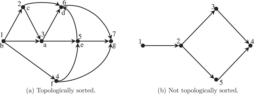
Figure 4.13Acyclic digraphs.
Topological sorting begins by finding a vertex of G = (V, E) with no outgoing edge (such a vertex must exist if G is acyclic) and assigning this vertex the highest number—namely, |V|. This vertex is then deleted from G, along with all its incoming edges. Since the remaining digraph is also acyclic, we can repeat the process and assign the next highest number, namely |V| − 1, to a vertex with no outgoing edges, and so on. To keep the algorithm O(|V| + |E|), we must avoid searching the modified digraph for a vertex with no outgoing edges.
We do so by performing a single depth-first search on the given acyclic digraph G. In addition to the usual array num, we will need another array, label, of size |V| for recording the topologically sorted vertex labels. That is, if there is an edge (u, v) in G, then label[u] < label[v]. The complete search and labeling procedure TOPSORT is given in Figure 4.14. Use the acyclic digraph in Figure 4.13a with vertex set V = {a, b, c, d, e, f, g} as the input to the topological sort algorithm in Figure 4.14; and verify that the vertices get relabeled 1 to 7, as shown next to the original names—in a correct topological order.

Figure 4.14Algorithm for topological sorting.
How to connect a given set of points with lowest cost is a frequently-encountered problem, which can be modeled as the problem of finding a minimum-weight spanning tree T in a weighted, connected, undirected graph G = (V, E). Methods for finding such a spanning tree, called a minimum spanning tree (MST), have been investigated in numerous studies and have a long history [11]. In this section we will discuss the bare essentials of the two commonly used MST algorithms—Kruskal’s and Prim’s—and briefly mention a third one.
An algorithm due to J. B. Kruskal, which employs the smallest-edge-first strategy, works as follows: First we sort all the edges in the given network by weight, in nondecreasing order. Then one by one the edges are examined in order, smallest to the largest. If an edge ei, upon examination, is found to form a cycle (when added to edges already selected) it is discarded. Otherwise, ei is selected to be included in the minimum spanning tree T. The construction stops when the required n − 1 edges have been selected or when all m edges have been examined. If the given network is disconnected, we would get a minimum spanning forest (instead of tree). More formally, Kruskal’s method may be stated as follows:
  T ← ϕ
  while |T| < (n−1) and E ≠ ϕ do
    e ← smallest edge in E
    E ← E − {e}
    if T ∪ {e} has no cycle then
      T ← T ∪ {e}
    end if
  end while
  if |T| < (n−1) then
     write ‘network disconnected’
  end if
Although the algorithm just outlined is simple enough, we do need to work out some implementation details and select an appropriate data structure for achieving an efficient execution.
There are two crucial implementations details that we must consider in this algorithm. If we initially sort all m edges in the given network, we may be doing a lot of unnecessary work. All we really need is to be able to to determine the next smallest edge in the network at each iteration. Therefore, in practice, the edges are only partially sorted and kept as a heap with smallest edge at the root of a min heap. In a graph with m edges, the initial construction of the heap would require O(m) computational steps; and the next smallest edge from a heap can be obtained in O (log m) steps. With this improvement, the sorting cost is O(m + p log m), where p is the number of edges examined before an MST is constructed. Typically, p is much smaller than m.
The second crucial detail is how to maintain the edges selected (to be included in the MST) so far, such that the next edge to be examined can be efficiently tested for a cycle formation.
As edges are examined and included in T, a forest of disconnected trees (i.e., subtrees of the final spanning tree) is produced. The edge e being examined will form a cycle if and only if both its end vertices belong to the same subtree in T. Thus to ensure that the edge currently being examined does not form a cycle, it is sufficient to check if it connects two different subtrees in T. An efficient way to accomplish this is to group the n vertices of the given network into disjoint subsets defined by the subtrees (formed by the edges included in T so far). Thus if we maintain the partially constructed MST by means of subsets of vertices, we can add a new edge by forming the UNION of two relevant subsets, and we can check for cycle formation by FINDing if the two end vertices of the edge, being examined, are in the same subset. These subsets can themselves be kept as rooted trees. The root is an element of the subset and is used as a name to identify that subset. The FIND subprocedure is called twice—once for each end vertex of edge e—to determine the sets to which the two end vertices belong. If they are different, the UNION subprocedure will merge the two subsets. (If they are the same subset, edge e will be discarded.)
The subsets, kept as rooted trees, are implemented by keeping an array of parent pointers for each of the n elements. Parent of a root, of course, is null. (In fact, it is useful to assign parent[root] = − number of vertices in the tree.) While taking the UNION of two subsets, we merge the smaller subset into the larger one by pointing the parent pointer in the root of the smaller subset to the root of the larger subset. Some of these details are shown in Figure 4.15. Note that r1 and r2 are the roots identifying the sets to which vertices u and v belong.

Figure 4.15Kruskal’s minimum spanning tree algorithm.
When algorithm in Figure 4.15 is applied to the weighted graph in Figure 4.16, the order in which edges are included one by one to form the MST are (3, 5), (4, 6), (4, 5), (4, 2), (6, 7), (3, 1). After the first five smallest edges are included in the MST, the 6th and 7th and 8th smallest edges are rejected. Then the 9th smallest edge (1, 3) completes the MST and the last two edges are ignored.
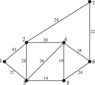
Figure 4.16A connected weighted graph for MST algorithm.
A second algorithm, discovered independently by several people (Jarnik in 1936, Prim in 1957, Dijkstra in 1959) employs the “nearest neighbor” strategy and is commonly referred to as Prim’s algorithm. In this method one starts with an arbitrary vertex s and joins it to its nearest neighbor, say y. That is, of all edges incident on vertex s, edge (s, y), with the smallest weight, is made part of the MST. Next, of all the edges incident on s or y we choose one with minimum weight that leads to some third vertex, and make this edge part of the MST. We continue this process of “reaching out” from the partially constructed tree (so far) and bringing in the “nearest neighbor” until all vertices reachable from s have been incorporated into the tree.
As an example, let us use this method to find the minimum spanning tree of the weighted graph given in Figure 4.16. Suppose that we start at vertex 1. The nearest neighbor of vertex 1 is vertex 3. Therefore, edge (1, 3) becomes part of the MST. Next, of all the edges incident on vertices 1 and 3 (and not included in the MST so far) we select the smallest, which is edge (3, 5) with weight 14. Now the partially constructed tree consists of two edges (1, 3) and (3, 5). Among all edges incident at vertices 1, 3, and 5, edge (5, 4) is the smallest, and is therefore included in the MST. The situation at this point is shown in Figure 4.17. Clearly, (4, 6), with weight 18 is the next edge to be included. Finally, edges (4, 2) and (6, 7) will complete the desired MST.

Figure 4.17Partially constructed MST for the network of Figure 4.16.
The primary computational task in this algorithm is that of finding the next edge to be included into the MST in each iteration. For each efficient execution of this task we will maintain an array near[u] for each vertex u not yet in the tree (i.e., u ∈ V − VT). near[u] is that vertex in VT which is closest to u. (Note that V is the set of all vertices in the network and VT is the subset of V included in MST thus far.) Initially, we set to indicate that s is in the tree, and for every other vertex v, .
For convenience, we will maintain another array dist[u] of the actual distance (i.e., edge weight) to that vertex in VT which is closest to u. In order to determine which vertex is to be added to the set VT next, we compare all nonzero values in dist array and pick the smallest. Thus n − i comparisons are sufficient to identify the ith vertex to be added. Initially, since s is the only vertex in VT, dist[u] is set to wsu. As the algorithm proceeds, these two arrays are updated in each iteration (see Figure 4.17 for an illustration).
A formal description of the nearest-neighbor algorithm is given in Figure 4.18. It is assumed that the input is given in the form of an n × n weight matrix W (in which nonexistent edges have ∞ weights). Set V = {1, 2,…, n} is the set of vertices of the graph. VT and ET are the sets of vertices and edges of the partially formed (minimum spanning) tree. Vertex set VT is identified by zero entries in array near.

Figure 4.18Prim’s minimum spanning tree algorithm.
There is yet a third method for computing a minimum spanning tree, which was first proposed by O. Boruvka in1,926(but rediscovered by G. Chouqet in 1938 and G. Sollin in 1961). It works as follows: First, the smallest edge incident on each vertex is found; these edges form part of the minimum spanning tree. There are at least ⌈n/2⌉ such edges. The connected components formed by these edges are collapsed into “supernodes” (There are no more than ⌊n/2⌋ such vertices at this point.) The process is repeated on “supernodes” and then on the resulting “supersupernodes,” and so on, until only a single vertex remains. This will require at most ⌊ log2 n⌋ steps, because at each step the number of vertices is reduced at least by a factor of 2. Because of its inherent parallelism the nearest-neighbor-from-each-vertex approach is particularly appealing for parallel implementations.
These three “greedy” algorithms and their variations have been implemented with different data structures and their relative performance—both theoretical as well as empirical—have been studied widely. The results of some of these studies can be found in [6, 12–14].
In many applications, the minimum spanning tree is required to satisfy an additional constraint, such as (i) the degree of each vertex in the MST should be equal to or less than a specified value; or (ii) the diameter of the MST should not exceed a specified value; or (iii) the MST must have at least a specified number of leaves (vertices of degree 1 in a tree); and the like. The problem of computing such a constrained minimum spanning tree is usually NP-complete. For a discussion of various constrained MST problems and some heuristics solving them see [15].
In the preceding section we dealt with the problem of connecting a set of points with smallest cost. Another commonly encountered and somewhat related problem is that of finding the lowest-cost path (called shortest path) between a given pair of points. There are many types of shortest-path problems. For example, determining the shortest path (i.e., the most economical path or fastest path, or minimum-fuel-consumption path) from one specified vertex to another specified vertex; or shortest paths from a specified vertex to all other vertices; or perhaps shortest path between all pairs of vertices. Sometimes, one wishes to find a shortest path from one given vertex to another given vertex that passes through certain specified intermediate vertices. In some applications, one requires not only the shortest but also the second and third shortest paths. Thus, the shortest-path problems constitute a large class of problems; particularly if we generalize it to include related problems, such as the longest-path problems, the most-reliable-path problems, the largest-capacity-path problems, and various routing problems. Therefore, the number of papers, books, reports, dissertations, and surveys dealing with the subject of shortest paths runs into hundreds [16].
Here we will discuss two very basic and important shortest-path problems: (i) how to determine the shortest distance (and a shortest path) from a specified vertex s to another specified vertex t, and (ii) how to determine shortest distances (and paths) from every vertex to every other vertex in the network. Several other problems can be solved using these two basic algorithms.
4.7.1Single-Source Shortest Paths, Nonnegative Weights
Let us first consider a classic algorithm due to Dijkstra for finding a shortest path (and its weight) from a specified vertex s (source or origin) to another specified vertex t (target or sink) in a network G in which all edge weights are nonnegative. The basic idea behind Dijkstra’s algorithm is to fan out from s and proceed toward t (following the directed edges), labeling the vertices with their distances from s obtained so far. The label of a vertex u is made permanent once we know that it represents the shortest possible distance from s (to u). All vertices not permanently labeled have temporary labels.
We start by giving a permanent label 0 to source vertex s, because zero is the distance of s from itself. All other vertices get labeled ∞, temporarily, because they have not been reached yet. Then we label each immediate successor v of source s, with temporary labels equal to the weight of the edge (s, v). Clearly, the vertex, say x, with smallest temporary label (among all its immediate successors) is the vertex closest to s. Since all edges have nonnegative weights, there can be no shorter path from s to x. Therefore, we make the label of x permanent. Next, we find all immediate successors of vertex x, and shorten their temporary labels if the path from s to any of them is shorter by going through x (than it was without going through x). Now, from among all temporarily labeled vertices we pick the one with the smallest label, say vertex y, and make its label permanent. This vertex y is the second closest vertex from s. Thus, at each iteration, we reduce the values of temporary labels whenever possible (by selecting a shorter path through the most recent permanently labeled vertex), then select the vertex with the smallest temporary label and make it permanent. We continue in this fashion until the target vertex t gets permanently labeled. In order to distinguish the permanently labeled vertices from the temporarily labeled ones, we will keep a boolean array final of order n. When the ith vertex becomes permanently labeled, the ith element of this array changes from false to true. Another array, dist, of order n will be used to store labels of vertices. A variable recent will be used to keep track of most recent vertex to be permanently labeled.
Assuming that the network is given in the form of a weight matrix W = [wij], with ∞ weights for nonexistent edges, and vertices s and t are specified, this algorithm (which is called Dijkstra’s shortest-path or the label-setting algorithm) may be described as follows (Figure 4.19).

Figure 4.19Dijkstra’s shortest-path algorithm.
4.7.2Single-Source Shortest Paths, Arbitrary Weights
In Dijkstra’s shortest-path algorithm (Figure 4.19), it was assumed that all edge weights wij were nonnegative numbers. If some of the edge weights are negative, Dijkstra’s algorithm will not work. (Negative weights in a network may represent costs and positive ones, profit.) The reason for the failure is that once the label of a vertex is made permanent, it cannot be changed in future iterations. In order to handle a network that has both positive and negative weights, we must ensure that no label is considered permanent until the program halts. Such an algorithm (called a label-correcting method, in contrast to Dijkstra’s label-setting method) is described as below.
Like Dijkstra’s algorithm, the label of the starting vertex s is set to zero and that of every other vertex is set to ∞, a very large number. That is, the initialization consists of
  dist(s) ← 0
  for all v ≠ s do
     dist(v) ← ∞
  end for
In the iterative step, dist(v) is always updated to the currently known distance from s to v, and the predecessor pred(v) of v is also updated to be the predecessor vertex of v on the currently known shortest path from s to v. More compactly, the iteration may be expressed as follows:
  while ∃ an edge (u,v) such that dist(u) + wu,v < dist(v) do
     dist(v) ← dist(u) + wu,v
     pred(v) ← u
  end while
Several implementations of this basic iterative step have been studied, experimented with, and reported in the literature. One very efficient implementation, works as follows.
We maintain a queue of “vertices to be examined.” Initially, this queue, Q, contains only the starting vertex s. The vertex u from the front of the queue is “examined” (as follows) and deleted. Examining u consists of considering all edges (u, v) going out of u. If the length of the path to vertex v (from s) is reduced by going through u, that is,
  if dist(u) + wu,v < dist(v) then
    dist(v) ← dist(u) + wu,v {// dist(v) is reset to the smaller value //}
    pred(v) ← u
  end if
Moreover, this vertex v is added to the queue (if it is not already in the queue) as a vertex to be examined later. Note that v enters the queue only if dist(v) is decremented as above and if v is currently not in the queue. Observe that unlike in Dijkstra’s method (the label-setting method) a vertex may enter (and leave) the queue several times—each time a shorter path is discovered. It is easy to see that the label-correcting algorithm will not terminate if the network has a cycle of negative weight.
We will now consider the problem of finding a shortest path between every pair of vertices in the network. Clearly, in an n-vertex directed graph there are n(n − 1) such paths—one for each ordered pair of distinct vertices—and n(n − 1)/2 paths in an undirected graph. One could, of course, solve this problem by repeated application of Dijkstra’s algorithm, once for each vertex in the network taken as the source vertex s. We will instead consider a different algorithm for finding shortest paths between all pairs of vertices, which is known as Warshall-Floyd algorithm. It requires computation time proportional to n3, and allows some of the edges to have negative weights, as long as no cycles of net negative weight exist.
The algorithm works by inserting one or more vertices into paths, whenever it is advantageous to do so. Starting with n × n weight matrix W = [wij] of direct distances between the vertices of the given network G, we construct a sequence of n matrices W(1), W(2),…, W(n). Matrix W(1), 1 ≤ l ≤ n, may be thought of as the matrix whose (i, j)th entry gives the length of the shortest path among all paths from i to j with vertices allowed as intermediate vertices. Matrix is constructed as follows:
(4.1) |
|---|
In other words, in iteration 1, vertex 1 is inserted in the path from vertex i to vertex j if wij > wi1 + w1j. In iteration 2, vertex 2 can be inserted, and so on.
For example, in Figure 4.6 the shortest path from vertex 2 to 4 is 2–1–3–4; and the following replacements occur:
Once the shortest distance is obtained in , the value of this entry will not be altered in subsequent operations.
We assume as usual that the weight of a nonexistent edge is ∞, that x + ∞ = ∞, and that for all x. It can easily be seen that all distance matrices W(l) calculated from Equation 4.1 can be overwritten on W itself. The algorithm may be stated as follows:
If the network has no negative-weight cycle, the diagonal entries represent the length of shortest cycles passing through vertex i. The off-diagonal entries are the shortest distances. Notice that negative weight of an individual edge has no effect on this algorithm as long as there is no cycle with a net negative weight.
Note that the algorithm in Figure 4.20 does not actually list the paths, it only produces their costs or weights. Obtaining paths is slightly more involved than it was in algorithm in Figure 4.19 where a predecessor array pred was sufficient. Here the paths can be constructed from a path matrix P = [pij] (also called optimal policy matrix), in which pij is the second to the last vertex along the shortest path from i to j—the last vertex being j. The path matrix P is easily calculated by adding the following steps in Figure 4.20. Initially, we set

Figure 4.20All-pairs shortest distance algorithm.
In the lth iteration if vertex l is inserted between i and j; that is, if wil + wlj < wij, then we set . At the termination of the execution, the shortest path (i, v1, v2,…, vq, j) from i to j can be obtained from matrix P as follows:
The storage requirement is n2, no more than for storing the weight matrix itself. Since all the intermediate matrices as well as the final distance matrix are overwritten on W itself. Another n2 storage space would be required if we generated the path matrix P also. The computation time for the algorithm in Figure 4.20 is clearly O(n3), regardless of the number of edges in the network.
4.8Eulerian and Hamiltonian Graphs
A path when generalized to include visiting a vertex more than once is called a trail. In other words, a trail is a sequence of edges (v1, v2), (v2, v3),…,(vk − 2, vk − 1), (vk − 1, vk) in which all the vertices (v1, v2,…, vk) may not be distinct but all the edges are distinct. Sometimes a trail is referred to as a (non-simple) path and path is referred to as a simple path. For example in Figure 4.8a (b, a), (a, c), (c, d), (d, a), (a, f) is a trail (but not a simple path because vertex a is visited twice.
If the first and the last vertex in a trail are the same, it is called a closed trail, otherwise an open trail. An Eulerian trail in a graph G = (V, E) is one that includes every edge in E (exactly once). A graph with a closed Eulerian trail is called a Eulerian graph. Equivalently, in an Eulerian graph, G, starting from a vertex one can traverse every edge in G exactly once and return to the starting vertex. According to a theorem proved by Euler in 1736, (considered the beginning of graph theory), a connected graph is Eulerian if and only if the degree of its every vertex is even.
Given a connected graph G it is easy to check if G is Eulerian. Finding an actual Eulerian trail of G is more involved. An efficient algorithm for traversing the edges of G to obtain an Euler trail was given by Fleury. The details can be found in Reference 4.
A cycle in a graph G is said to be Hamiltonian if it passes through every vertex of G. Many families of special graphs are known to be Hamiltonian, and a large number of theorems have been proved that give sufficient conditions for a graph to be Hamiltonian. However, the problem of determining if an arbitrary graph is Hamiltonian is NP-complete.
Graph theory, a branch of combinatorial mathematics, has been studied for over two centuries. However, its applications and algorithmic aspects have made enormous advances only in the past fifty years with the growth of computer technology and operations research. Here we have discussed just a few of the better-known problems and algorithms. Additional material is available in the references provided. In particular, for further exploration the Stanford GraphBase [17], the LEDA [18], and the Graph Boost Library [19] provide valuable and interesting platforms with collection of graph-processing programs and benchmark databases.
The author gratefully acknowledges the help provided by Hemant Balakrishnan in preparing this chapter.
1.R. K. Ahuja, T. L. Magnanti, and J. B. Orlin, Network Flows: Theory, Algorithms, and Applications, Prentice Hall, 1993.
2.N. Deo, Graph Theory with Applications in Engineering and Computer Science, Prentice-Hall, 1974.
3.M. M. Syslo, N. Deo, and J. S. Kowalik, Discrete Optimization Algorithms: With Pascal Programs, Prentice-Hall, 1983.
4.K. Thulasiraman and M. N. S. Swamy, Graphs: Theory and Algorithms, Wiley-Interscience, 1992.
5.E. M. Reingold, J. Nievergelt, and N. Deo, Combinatorial Algorithms: Theory and Practice, Prentice-Hall, 1977.
6.R. Sedgewick, Algorithms in C: Part 5 Graph Algorithms, Addison-Wesley, third edition, 2002.
7.H. N. Gabow, Path-based depth-first search for strong and biconnected components, Information Processing, Vol. 74, pp. 107–114, 2000.
8.R. E. Tarjan, Data Structures and Network Algorithms, Society for Industrial and Applied Mathematics, 1983.
9.T. H. Cormen, C. L. Leiserson, and R. L. Rivest, Introduction to Algorithms, MIT Press and McGraw-Hill, 1990.
10.E. Horowitz, S. Sahni, and B. Rajasekaran, Computer Algorithms/C++, Computer Science Press, 1996.
11.R. L. Graham and P. Hell, On the history of minimum spanning tree problem, Annals of the History of Computing, Vol. 7, pp. 43–57, 1985.
12.B. Chazelle, A minimum spanning tree algorithm with inverse Ackermann type complexity, Journal of the ACM, Vol. 47, pp. 1028–1047, 2000.
13.B. M. E. Moret and H. D. Shapiro, An empirical analysis of algorithms for constructing minimum spanning tree, Lecture Notes on Computer Science, Vol. 519, pp. 400–411, 1991.
14.C. H. Papadimitriou and K. Steiglitz, Combinatorial Optimization: Algorithms and Complexity, Rentice-Hall, 1982.
15.N. Deo and N. Kumar, Constrained spanning tree problem: Approximate methods and parallel computation, American Math Society, Vol. 40, pp. 191–217, 1998.
16.N. Deo and C. Pang, Shortest path algorithms: Taxonomy and annotation, Networks, Vol. 14, pp. 275–323, 1984.
17.D. E. Knuth, The Stanford GraphBase: A Platform for Combinatorial Computing, Addison-Wesley, 1993.
18.K. Mehlhorn and S. Naher, LEDA: A Platform for Combinatorial and Geometric Computing, Cambridge University Press, 1999.
19.J. G. Siek, L. Lee, and A. Lumsdaine, The Boost Graph Library—User Guide and Reference Manual, Addison Wesley, 2002.
20.K. Mehlhorn, Data Structures and Algorithms 2: NP-Completeness and Graph Algorithms, Springer-Verlag, 1984.
*This chapter has been reprinted from first edition of this Handbook, without any content updates.