
S. S. Iyengar
Florida International University
V. K. Vaishnavi†
Georgia State University
S. Gunasekaran†
Louisiana State University
What is a Quadtree?•Variants of Quadtrees
Compact Quadtrees•Forest of Quadtrees (FQT)
58.7Translation Invariant Data Structure (TID)
58.8Content-Based Image Retrieval System
What is CBIR?•An Example of CBIR System
Image has been an integral part of our communication. Visual information aids us in understanding our surroundings better. Image processing, the science of manipulating digital images, is one of the methods used for digitally interpreting images. Image processing generally comprises three main steps:
1.Image acquisition: Obtaining the image by scanning it or by capturing it through some sensors.
2.Image manipulation/analysis: Enhancing and/or compressing the image for its transfer or storage.
3.Display of the processed image.
Image processing has been classified into two levels: low-level image processing and high-level image processing. Low-level image processing needs little information about the content or the semantics of the image. It is mainly concerned with retrieving low-level descriptions of the image and processing them. Low-level data include matrix representation of the actual image. Image calibration and image enhancement are examples of low-level image processing.
High-level image processing is basically concerned with segmenting an image into objects or regions. It makes decisions according to the information contained in the image. High-level data are represented in symbolic form. The data include features of the image such as object size, shape and its relation with other objects in the image. These image-processing techniques depend significantly on the underlying image data structure. Efficient data structures for region representation are important for use in manipulating pictorial information.
Many techniques have been developed for representing pictorial information in image processing [1]. These techniques include data structures such as quadtrees, linear quadtrees, Forest of Quadtrees, and Translation Invariant Data structure (TID). We will discuss these data structures in the following sections. Research on quadtrees has produced several interesting results in different areas of image processing [2–7]. In 1981, Jones and Iyengar [8] proposed methods of refining quadtrees. A good tracing of the history of the evolution of quadtrees is provided by Klinger and Dyer [9]. See also Chapter 20 of this handbook.
An image is a visual reproduction of an object using an optical or electronic device. Image data include pictures taken by satellites, scanned images, aerial photographs and other digital photographs. In the computer, image is represented as a data file that consists of a rectangular array of picture elements called pixels. This rectangular array of pixels is also called a raster image. The pixels are the smallest programmable visual unit. The size of the pixel depends on the resolution of the monitor. The resolution can be defined as the number of pixels present on the horizontal axis and vertical axis of a display monitor. When the resolution is set to maximum the pixel size is equal to a dot on the monitor. The pixel size increases with the decrease of the resolution. Figure 58.1 shows an example of an image.

Figure 58.1Example of an image.
In a monochrome image each pixel has its own brightness value ranging from 0 (black) to 255 (white). For a color image each pixel has a brightness value and a RGB color value. RGB is an additive color state that has separate values for red, green, and blue. Hence each pixel has independent values (0–255) for red, green, and blue colors. If the values for red, green, and blue components of the pixel are the same then the resulting pixel color is gray. Different shades of gray pixels constitute a gray-scale image. If pixels of an image have only two states, black or white, then the image is called a binary image.
Image data can be classified into raster graphics and vector graphics. Raster graphics, also known as bitmap graphics, represents an image using x and y coordinates (for 2d-images) of display space; this grid of x and y coordinates is called the raster. Figure 58.2 shows how a circle will appear in raster graphics. In raster graphics an image is divided up in raster. All raster dots that are more than half full are displayed as black dots and the rest as white dots. This results in step like edges as shown in the figure. The appearance of jagged edges can be minimized by reducing the size of the raster dots. Reducing the size of the dots will increase the number of pixels needed but increases the size of the storage space.

Figure 58.2A circle in raster graphics.
Vector graphics uses mathematical formulas to define the image in a two-dimensional or three-dimensional space. In a vector graphics file an image is represented as a sequence of vector statements instead of bits, as in bitmap files. Thus it needs just minimal amount of information to draw shapes and therefore the files are smaller in size compared to raster graphics files.
Vector graphics does not consist of black and white pixels but is made of objects like line, circle, and rectangle. The other advantage of vector graphics is that it is flexible, so it can be resized without loss of information. Vector graphics is typically used for simple shapes. CorelDraw images, PDF, and PostScript are all in vector image format. The main drawbacks of vector graphics is that it needs longer computational time and has very limited choice of shapes compared to raster graphics.
Raster file, on the other hand, is usually larger than vector graphics file and is difficult to modify without loss of information. Scaling a raster file will result in loss of quality whereas vector graphics can be scaled to the quality of the device on which it is rendered. Raster graphics is used for representing continuous numeric values unlike vector graphics, which is used for discrete features. Examples of raster graphic formats are GIF, JPEG, and PNG.
Considerable research on quadtrees has produced several interesting results in different areas of image processing. The basic relationship between a region and its quadtree representation is presented in [3]. In 1981, Jones and Iyengar [8] proposed methods for refining quadtrees. The new refinements were called virtual quadtrees, which include compact quadtrees and forests of quadtrees. We will discuss virtual quadtrees in a later section of this chapter. Much work has been done on the quadtree properties and algorithms for manipulations and translations have been developed by Samet [10,11], Dyer [2] and others [3,5,12].
A quadtree is a class of hierarchical data structures used for image representation. The fundamental principle of quadtrees is based on successive regular decomposition of the image data until each part contains data that is sufficiently simple so that it can be represented by some other simpler data structure. A quadtree is formed by dividing an image into four quadrants, each quadrant may further be divided into four sub quadrants and so on until the whole image has been broken down to small sections of uniform color.
In a quadtree the root represents the whole image and the non-root nodes represent sub quadrants of the image. Each node of the quadtree represents a distinct section of the image; no two nodes can represent the same part of the image. In other words, the sub quadrants of the image do not overlap. The node without any child is called a leaf node and it represents a region with uniform color. Each non-leaf node in the tree has four children, each of which represents one of the four sub regions, referred to as NW, NE, SW, and SE, that the region represented by the parent node is divided into.
The leaf node of a quadtree has the color of the pixel (black or white) it is representing. The nodes with uniform colored children have the color of their children and all their child nodes are removed from the tree. All the other nodes with non-uniform colored children have the gray color. Figure 58.3 shows the concept of quadtrees.

Figure 58.3The concept of quadtrees.
The image can be retrieved from the quadtree by using a recursive procedure that visits each leaf node of the tree and displays its color at an appropriate position. The procedure starts with visiting the root node. In general, if the visited node is not a leaf then the procedure is recursively called for each child of the node, in order from left to right.
The main advantage of the quadtree data structure is that images can be compactly represented by it. The data structure combines data having similar values and hence reduces storage size. An image having large areas of uniform color will have very small storage size. The quadtree can be used to compress bitmap images, by dividing the image until each section has the same color. It can also be used to quickly locate any object of interest.
The drawback of the quadtree is that it can have totally different representation for images that differ only in rotation or translation. Though the quadtree has better storage efficiency compared to other data structures such as the array, it also has considerable storage overheads. For a given image it stores many white leaf nodes and intermediate gray nodes, which are not required information.
The numerous quadtree variants that have been developed so far can be differentiated by the type of data they are designed to represent [13]. The many variants of the quadtree include region quadtrees, point quadtrees, line quadtrees, and edge quadtrees. Region quadtrees are meant for representing regions in images, while point quadtrees, edge quadtrees, and line quadtrees are used to represent point features, edge features, and line features, respectively. Thus there is no single quadtree data structure which is capable of representing a mixture of features of images like regions and lines.
58.3.2.1Region Quadtrees
In the region quadtree, a region in a binary image is a subimage that contains either all 1’s or all 0’s. If the given region does not consist entirely of 1’s or 0’s, then the region is divided into four quadrants. This process is continued until each divided section consists entirely of 1’s or 0’s; such regions are called final regions. The final regions (either black or white) are represented by leaf nodes. The intermediate nodes are called gray nodes. A region quadtree is space efficient for images containing square-like regions. It is very inefficient for regions that are elongated or for representing line features.
58.3.2.2Line Quadtrees
The line quadtree proposed by Samet [14] is used for representing the boundaries of a region. The given region is represented as in the region quadtree with additional information associated with nodes representing the boundary of the region. The data structure is used for representing curves that are closed. The boundary following algorithm using the line quadtree data structure is at least twice as good as the one using the region quadtree in terms of execution time; the map superposition algorithm has execution time proportional to number of nodes in the line quadtree [13]. The main disadvantage of the line quadtree is that it cannot represent independent linear features.
58.3.2.3Edge Quadtrees
Shneier [15] formulated the edge quadtree data structure for storing linear features. The main principle used in the data structure is to approximate the curve being represented by a number of straight line segments. The edge quadtree is constructed using a recursive procedure. If the sub quadrant represented by a node does not contain any edge or line, it is not further subdivided and is represented by a leaf. If it does contain one then an approximate equation is fitted to the line. The error caused by approximation is calculated using a measure such as least squares. When the error is less than the predetermined value, the node becomes a leaf; otherwise the region represented by the node is further subdivided. If an edge terminates (within the region represented by) a node then a special flag is set. Each node contains magnitude, direction, intercept, and error information about the edge passing through the node. The main drawback of the edge quadtree is that it cannot efficiently handle two or more intersecting lines.
58.3.2.4Template quadtrees
An image can have regions and line features together. The above quadtree representational schemas are not efficient for representing such an image in one quadtree data structure. The template quadtree is an attempt toward development of such a quadtree data structure. It was proposed by Manohar, Rao, and Iyengar [13] to represent regions and curvilinear data present in images.
A template is a 2k × 2k sub image, which contains either a region of uniform color or straight run of black pixels in horizontal, vertical, left diagonal, or right diagonal directions spanning the entire sub image. All the possible templates for a 2×2 sub image are shown in Figure 58.4.

Figure 58.4Template sets.
A template quadtree can be constructed by comparing a quadrant with any one of the templates, if they match then the quadrant is represented by a node with the information about the type of template it matches. Otherwise the quadrant is further divided into four sub quadrants and each one of them is compared with any of the templates of the next lower size. This process is recursively followed until the entire image is broken down into maximal blocks corresponding to the templates. The template quadtree representation of an image is shown in Figure 58.5.

Figure 58.5Template quadtree representation.
Here the leaf is defined as a template of variable size, therefore it does not need any approximation for representing curves present in the images. The advantage of template quadtree is that it is very accurate and has the capabilities for representing features like regions and curves. The main drawback is that it needs more space compared to edge quadtrees. For more information on template quadtrees see Reference 13.
The quadtree has become a major data structure in image processing. Though the quadtree has better storage efficiency compared to other data structures such as the array, it also has considerable storage overhead. Jones and Iyengar [16] have proposed two ways in which quadtrees may be efficiently stored: as “forest of quadtrees” and as “compact quadtrees.” They called these new data structures virtual quadtrees because the basic operations performed in quadtrees can also be performed on the new representations. The virtual quadtree is a space-efficient way of representing a quadtree. It is a structure that simulates quadtrees in such a way that we can,
1.Determine the color of any node in the quadtree.
2.Find the child node of any node, in any direction in the quadtree.
3.Find the parent node of any node in the quadtree.
The two types of virtual quadtrees, which we are going to discuss, are the compact quadtree and the forest of quadtrees.
The compact quadtree has all the information contained in a quadtree but needs less space. It is represented as C(T), where T is the quadtree it is associated with. Each set of four sibling nodes in the quadtree is represented as a single node called metanode in the corresponding compact quadtree.
The metanode M has four fields, which are explained as follows:
•MCOLOR(M, D)—The colors of the nodes included in M. Where D ∈ {NW,NE,SW,SE}.
•MSONS(M)—Points to the first metanode that represents offsprings of a node represented in M; NIL if no offspring exists.
•MFATHER(M)—Points to the metanode that holds the representation of the parent of the nodes that M represents.
•MCHAIN(M)—If there are more than one metanode that represent offspring of nodes represented by a given metanode M, then these are linked by MCHAIN field.
The compact quadtree for the quadtree shown in the Figure 58.6 is given in Figure 58.7. In Figure 58.7 downward links are MSON links, horizontal links are MCHAIN links and upward links are MFATHER links.

Figure 58.6Quadtree with coordinates.
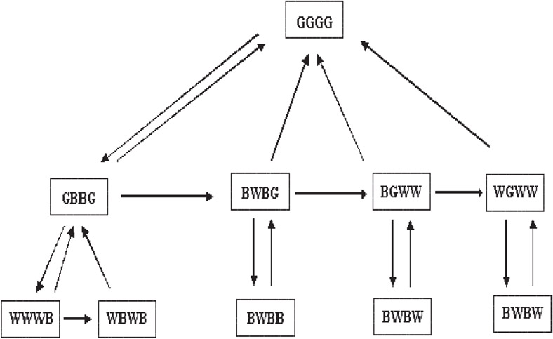
Figure 58.7Compact quadtree C(T).
The compact quadtree uses the same amount of space for the storage of color but it uses very less space for storage of pointers. In Figure 58.7, the compact quadtree has 10 metanodes, whereas the quadtree has 41 nodes. Thus it saves about 85% of the storage space. Since the number of nodes in a compact quadtree is less a simple recursive tree traversal can be done more efficiently.
58.4.2Forest of Quadtrees (FQT)
Jones and Iyengar [8] proposed a variant of quadtrees called forest of quadtrees to improve the space efficiency of quadtrees. A forest of quadtrees is represented by F(T) where T is the quadtree it represents. A forest of quadtrees, F(T) that represents T consists of a table of triples of the form (L, K, P), and a collection of quadtrees where,
1.Each triple (L, K, P) consists of the coordinates, (L, K), of a node in T, and a pointer, P, to a quadtree that is identical to the subtree rooted at position (L, K) in T.
2.If (L, K) and (M, N) are coordinates of nodes recorded in F(T), then neither node is a descendant of the other.
3.Every black leaf in T is represented by a black leaf in F(T).
To obtain the corresponding forest of quadtrees, the nodes in a quadtree need to be classified as good and bad nodes. A leaf node with black color or an intermediate node that has two or more black child nodes are called good nodes, the rest are called bad nodes. Only the good nodes are stored in the forest of quadtrees thereby saving lot of storage space. Figure 58.8 contains a forest of quadtrees that represents the quadtree shown in Figure 58.6.

Figure 58.8Forest of quadtrees F(T).
To reduce a quadtree to a forest of quadtrees, we first need to identify the good nodes and the bad nodes. We then break down the quadtree into smaller quadtrees in such a way that each of them has a good root node and none of them is a subtree of another and the bad nodes encountered by forest are freed. This collection of quadtrees is called as forest of quadtrees. The time required for the execution of the conversion is obviously linear in the number of nodes in the quadtree [16].
Theorem:
The maximum number of trees in a forest of quadtrees derived from a quadtree that represents a square of dimension 2k × 2k is 4k − 1, that is, one-fourth the area of the square. For proof see Reference 16.
The corresponding quadtree can be easily reconstructed from a forest of quadtrees F. The reconstructed quadtree R(F) consists of real nodes and virtual nodes (nodes corresponding to the bad nodes that are deleted while creating the forest). Since the virtual nodes require no storage they are located by giving their coordinates. The virtual nodes are represented as v(L, K).
Quadtrees and R-trees [17] are two commonly used spatial data structures to locate or organize objects in a given image. Both quadtrees and R-trees use bounding boxes to depict the outline of the objects. Therefore, the data structure only needs to keep track of the boundaries instead of the actual shape and size of the objects in the image. The size of the bounding boxes usually depends on the size of the object we are trying to locate.
The R-tree (see also Chapter 22) is a hierarchical, height balanced data structure, similar to the B+-tree that aggregates objects based on their spatial proximity. It is a multidimensional generalization of the B+-tree. The R-tree indexes multidimensional data objects by enclosing data objects in bounding rectangles, which may further be enclosed in bounding rectangles; these bounding rectangles can overlap each other. Each node except the leaf node has a pointer and the corresponding bounding rectangle. The pointer points to the subtree with all the objects enclosed in its corresponding rectangle. The leaf node has a bounding rectangle and the pointer pointing to the actual data object. The root node has a minimum of two children unless it is a leaf node and all the leaf nodes appear at the same level. Figure 58.9 Shows the R-tree representation of an image.

Figure 58.9The concept of R-tree.
The main difference between quadtrees and R-trees is that unlike R-trees the bounding rectangle of quadtrees do not overlap. In real world objects overlap; in such cases more than one node in a quadtree can point to the same object. This is a serious disadvantage for the quadtree. Figure 58.10 shows the quadtree representation of the image in Figure 58.9.

Figure 58.10Quadtree representation of the image in Figure 58.9.
As you can see from the Figure 58.10 objects like “C” and “D” are represented by more than one node. This makes it difficult to find the origin of the quadtree.
The R-tree is a dynamic structure, so its contents can be modified without having to reconstruct the entire tree. It can be used to determine which objects intersect a given query region. The R-tree representation of an image is not unique; size and placement of rectangles in the tree depends on the sequence of insertions and deletions resulting in the tree starting from the empty R-tree.
Octrees are 3D equivalent of quadtrees and are used for representing 3D images. An octree is formed by dividing a 3D space into 8 sub-cubes called cells. This process of dividing the cube into cells is carried on until the (image) objects lie entirely inside or outside the cells. The root node of an octree represents a cube, which encompasses the objects of interest.
In the octree each node except the leaf node has eight child nodes, which represent the sub-cubes of the parent node. The node stores information like pointer to the child nodes, pointer to the parent node, and pointers to the contents of the cube. An example of an octree representation is shown in Figure 58.11.

Figure 58.11Octree representation.
The Octree become very ineffective if the objects in the image that it is representing are not uniformly distributed, as in that case many nodes in the octree will not contain any objects. Such an octree is also very costly to compute as a large amount of data has to be examined.
58.7Translation Invariant Data Structure (TID)
Methods for the region representation using quadtrees exist in the literature [2,10,18]. Much work has been done on quadtree properties, and algorithms for translations and manipulations have been derived by Dyer [2], Samet [11,19], Shneier [20] and others.
Various improvements to quadtrees have been suggested including forests of quadtrees, hybrid quadtrees, linear quadtrees, and optimal quadtrees for image segments. All of these methods try to optimize quadtrees by removing some are all of the gray and white nodes. All of them maintain the same number of black nodes.
All these methods are sensitive to the placement of the origin. An image, which has been translated from its original position, can have a very different looking structure [21]. We explain this phenomenon by using the example given in Figure 58.12. In Example 1, the black square is in the upper left corner. In Example 2, it is translated down and right by one pixel. Figure 58.13 gives the quadtree representation for these two examples.

Figure 58.12Sample Regions.

Figure 58.13Quadtrees for Example 1 and 2 of Figure 58.12.
The shift sensitivity of the image data structure derives from the fact that the positions of the maximal blocks represented by leaf nodes are not explicitly represented in the data structure. Instead, these positions are determined by the paths leading to them from the root of the tree. Thus, when the image is shifted, the maximal blocks are formed in a different way.
For this reason Scott and Iyengar [21] have introduced a new data structure called Translation Invariant Data structure (TID), which is not sensitive to the placement of the region and is translation invariant.
A maximal square is a black square of pixels that is not included in any large square of black pixels. TID is made of such maximal squares, which are represented as (i, j, s) where (i, j) is the coordinates of the northwest vertex of the square and “s” is the length of the square. Translation made to any image can be represented as a function of these triples. For example consider a triple (i, j, s), translating it x units to the right and y units up yields (i+x, j+y, s) [21].
The rotation of the square by π/2 is only slightly more complicated due to the fact that the NW corner of the square changes upon rotation. The π/2 rotation around the origin gives (− j, i +s, s).
58.8Content-Based Image Retrieval System
Images have always been a part of human communication. Due to the increase in the use of Internet the interest in the potential of digital images has increased greatly. Therefore we need to store and retrieve images in an efficient way. Locating and retrieving a desired image from a large database can be a very tedious process and is still an active area of research. This problem can be reduced greatly by using Content-Based Image Retrieval (CBIR) systems, which retrieves images based only on the content of the image. This technique retrieves images on the basis of automatically-derived features such as color, texture, and shape.
Content-Based Image Retrieval is a process of retrieving desired images from a large database based on the internal features that can be obtained automatically from the images themselves. CBIR techniques are used to index and retrieve images from databases based on their pictorial content, typically defined by a set of features extracted from an image that describe the color, texture, and/or shape of the entire image or of specific objects in the image. This feature description is used to index a database through various means such as distance-based techniques, rule-based decision-making, and fuzzy inferencing [22–24]. Images can be matched in two ways. Firstly, an image can be compared with another image to check for similarity. Secondly, images similar to the given image can be retrieved by searching a large image database. The latter process is called content-based image retrieval.
58.8.1.1General Structure of CBIR Systems
The general computational framework of a CBIR system as shown in Figure 58.14 was proposed in Reference 25.
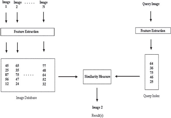
Figure 58.14Computational framework of CBIR systems.
At first, the image database is created, which stores the images as numerical values supplied by the feature extraction algorithms. These values are used to locate an image similar to the query image. The query image is processed by the same feature extraction algorithm that is applied to the images stored in the database.
The similarity between the query image and the images stored in the database can be verified with the help of the similarity measure algorithm, which compares the results obtained from the feature extraction algorithms for both the query image and the images in the database. Thus after comparing the query image with all the images in the database the similarity measure algorithm gives a set as the result, which has all the images from the database that are similar to the query image.
58.8.2An Example of CBIR System
An example of Content-Based Image Retrieval System is BlobWorld. The BlobWorld system, developed at the University of California, Berkeley, supports color, shape, spatial, and texture matching features. Blobworld is based on finding coherent image regions that roughly correspond to objects. The system automatically separates each image into homogeneous regions in order to improve content-based image retrieval. Querying is based on the user specifying attributes of one or two regions of interest, rather than a description of the entire image. For more information on Blobworld see Reference 26.
CBIR techniques are likely to be of most use in restricted subject areas, where merging with other types of data like text and sound can be achieved. Content-based image retrieval provides an efficient solution to the restrictions and the problems caused by the traditional information retrieval technique. The number of active research systems is increasing, which reflects the increasing interest in the field of content-based image retrieval.
In this chapter we have explained what an image data is and how it is stored in raster graphics and vector graphics. We then discussed some of the image representation techniques like quadtrees, virtual quadtrees, octrees, R-trees and translation invariant data structures. Finally, we have given a brief introduction to Content-Based Image Retrieval (CBIR) systems. For more information on image retrieval concepts see References 22–25.
The authors acknowledge the contributions of Sridhar Karra and all the previous collaborators in preparing this chapter.
1.H. Samet, The Design and Analysis of Spatial Data Structures. Addison-Wesley Pub. Co., 1990.
2.C. R. Dyer, A. Rosenfeld, H. Samet, Region Representation: Boundary Codes from Quadtrees, Communication of the ACM, 23, 1980, 171–179.
3.G. M. Hunter and K. Steiglitz, Operations on Images Using Quadtrees, IEEE Transactions on Pattern Analysis and Machine Intelligence, 1(2), April 1979, 145–153.
4.G. M. Hunter and K. Steiglitz, Linear Transformation of Pictures Represented By Quadtrees, Computer, Graphics and Image Processing, 10(3), July 1979, 289–296.
5.E. Kawaguchi and T. Endo, On a Method of Binary-Picture Representation and Its Application to Data Compression, IEEE Transactions on Pattern Analysis and Machine Intelligence, 2(1), January 1980, 27–35.
6.A. Klinger, Patterns and Search Statistics, Optimizing Methods in Statistics, J. D. Rustagi, (Ed.), Academic Press, New York, 1971.
7.A. Klinger and M. L. Rhodes, Organization and Access of Image Data by Areas, IEEE Transactions on Pattern Analysis and Machine Intelligence, 1(11), January 1979, 50–60.
8.L. Jones and S. S. Iyengar, Representation of a Region as a Forest of Quadtrees, Proc. IEEE-PRIP 81 Conference, TX, IEEE Publications, 57–59.
9.A. Klinger and C. R. Dyer, Experiments in Picture Representation Using Regular Decomposition, Computer Graphics and Image Processing, 5(1), March 1976, 68–105.
10.H. Samet, Region Representation: Quadtree from Boundary Codes, Communications of the ACM, 23(3), March 1980, 163–170.
11.H. Samet, Connected Component Labeling using Quadtrees, JACM, 28(3), July 1981, 487–501.
12.L. Jones and S. S. Iyengar, Virtual Quadtrees, Proc. IEEE-CVIP 83 Conference, Virginia, IEEE Publications101–105.
13.M. Manohar, P. Sudarsana Rao, S. Sitarama Iyengar, Template Quadtrees for Representing Region and Line Data Present in Binary Images, NASA Goddard Flight Center, Greenbelt, MD, 1988.
14.H. Samet and R. E. Webber, On Encoding Boundaries with Quadtrees, IEEE Transcations on Pattern Analysis and Machine Intelligence, 6, 1984, 365–369.
15.Edge Pyramids and Edge Quadtrees, Computer Graphics and Image Process, 17, 1981, 211–224.
16.L. P. Jones and S. S. Iyengar, Space and Time Efficient Virtual Quadtrees, IEEE Transactions on Pattern Analysis and Machine Intelligence, 6(2), March 1984, 244–247.
17.A. Guttman, R-Trees: A Dynamic Index Structure for Spatial Searching, Proceedings of the SIGMOD Conference, 47–57.
18.H. Samet, Region Representation: Quadtree from Binary Arrays, Computer Graphics Image Process, 18(1), 1980, 88–93.
19.H. Samet, An Algorithm for Converting Rasters to Quadtrees, IEEE Transcations on Pattern Analysis and Machine Intelligence, 3(1), January 1981, 93–95.
20.M. Shneier, Path Length Distances for Quadtrees, Information Sciences, 23(1), 1981, 49–67.
21.D. S. Scott and S. S. Iyengar, TID- A Translation Invariant Data Structure For Storing Images, Communications of the ACM, 29(5), May 1985, 418–429.
22.C. Hsu, W. W. Chu, and R. K. Taira, A Knowledge-Based Approach for Retrieving Images by Content, IEEE Transcations on Knowledge and Data Engineering, 8(4), August 1996.
23.P. W. Huang and Y. R. Jean, Design of Large Intelligent Image Database Systems, International Journal of Intelligent Systems, 11, 1996, 347.
24.B. Tao and B. Dickinson, Image Retrieval and Pattern Recognition, The International Society for Optical Engineering, 2916, 1996, 130.
25.J. Zachary, S. S. Iyengar, J. Barhen, Content Based Image Retrieval and Information Theory, A General Approach, JASIS.
26.C. Carson, M. Thomas, S. Belongie, J. M. Hellerstein, J. Malik, Blobworld: A System for Region-based Image Indexing and Retrieval, Proc. Int’l Conf. Visual Information System, 509–516.
*This chapter has been reprinted from first edition of this Handbook, without any content updates.
†We have used this author’s affiliation from the first edition of this handbook, but note that this may have changed since then.