
Sartaj Sahni
University of Florida
8.1Definition and an Application
Inserting an Element•Removing the Min Element•Initializing an Interval Heap•Complexity of Interval Heap Operations•The Complementary Range Search Problem
Inserting an Element•Removing the Min Element
Inserting an Element•Removing the Min Element
Dual Priority Queues•Total Correspondence•Leaf Correspondence
8.1Definition and an Application
A double-ended priority queue (DEPQ) is a collection of zero or more elements. Each element has a priority or value. The operations performed on a double-ended priority queue are:
1.getMin() …return element with minimum priority
2.getMax() …return element with maximum priority
3.put(x) …insert the element x into the DEPQ
4.removeMin() …remove an element with minimum priority and return this element
5.removeMax() …remove an element with maximum priority and return this element
One application of a DEPQ is to the adaptation of quick sort, which has the the best expected run time of all known internal sorting methods, to external sorting. The basic idea in quick sort is to partition the elements to be sorted into three groups L, M, and R. The middle group M contains a single element called the pivot, all elements in the left group L are ≤ the pivot, and all elements in the right group R are ≥ the pivot. Following this partitioning, the left and right element groups are sorted recursively.
In an external sort, we have more elements than can be held in the memory of our computer. The elements to be sorted are initially on a disk and the sorted sequence is to be left on the disk. When the internal quick sort method outlined above is extended to an external quick sort, the middle group M is made as large as possible through the use of a DEPQ. The external quick sort strategy is:
1.Read in as many elements as will fit into an internal DEPQ. The elements in the DEPQ will eventually be the middle group of elements.
2.Read in the remaining elements. If the next element is ≤ the smallest element in the DEPQ, output this next element as part of the left group. If the next element is ≥ the largest element in the DEPQ, output this next element as part of the right group. Otherwise, remove either the max or min element from the DEPQ (the choice may be made randomly or alternately); if the max element is removed, output it as part of the right group; otherwise, output the removed element as part of the left group; insert the newly input element into the DEPQ.
3.Output the elements in the DEPQ, in sorted order, as the middle group.
4.Sort the left and right groups recursively.
In this chapter, we describe four implicit data structures—symmetric min-max heaps, interval heaps, min-max heaps, and deaps—for DEPQs. Also, we describe generic methods to obtain efficient DEPQ data structures from efficient data structures for single-ended priority queues (PQ).*
Several simple and efficient implicit data structures have been proposed for the representation of a DEPQ [1–7]. All of these data structures are adaptations of the classical heap data structure (Chapter 2) for a PQ. Further, in all of these DEPQ data structures, getMax and getMin take O(1) time and the remaining operations take O(log n) time each (n is the number of elements in the DEPQ). The symmetric min-max heap structure of Arvind and Pandu Rangan [1] is the simplest of the implicit data structures for DEPQs. Therefore, we describe this data structure first.
A symmetric min-max heap (SMMH) is a complete binary tree in which each node other than the root has exactly one element. The root of an SMMH is empty and the total number of nodes in the SMMH is n + 1, where n is the number of elements. Let x be any node of the SMMH. Let elements(x) be the elements in the subtree rooted at x but excluding the element (if any) in x. Assume that elements. x satisfies the following properties:
1.The left child of x has the minimum element in elements(x).
2.The right child of x (if any) has the maximum element in elements(x).
Figure 8.1 shows an example SMMH that has 12 elements. When x denotes the node with 80, elements(x) = {6, 14, 30, 40}; the left child of x has the minimum element 6 in elements(x); and the right child of x has the maximum element 40 in elements(x). You may verify that every node x of this SMMH satisfies the stated properties.
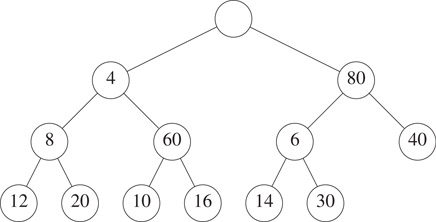
Figure 8.1A symmetric min-max heap.
Since an SMMH is a complete binary tree, it is stored as an implicit data structure using the standard mapping of a complete binary tree into an array. When n = 1, the minimum and maximum elements are the same and are in the left child of the root of the SMMH. When n > 1, the minimum element is in the left child of the root and the maximum is in the right child of the root. So the getMin and getMax operations take O(1) time.
It is easy to see that an n + 1-node complete binary tree with an empty root and one element in every other node is an SMMH iff the following are true:
Pl: For every node x that has a right sibling, the element in x is less than or equal to that in the right sibling of x.
P2: For every node x that has a grandparent, the element in the left child of the grandparent is less than or equal to that in x.
P3: For every node x that has a grandparent, the element in the right child of the grandparent is greater than or equal to that in x.
Notice that if property P1 is satisfied at node x, then at most one of P2 and P3 may be violated at x. Using properties P1 through P3 we arrive at simple algorithms to insert and remove elements. These algorithms are simple adaptations of the corresponding algorithms for min and max heaps. Their complexity is O(log n). We describe only the insert operation. Suppose we wish to insert 2 into the SMMH of Figure 8.1. Since an SMMH is a complete binary tree, we must add a new node to the SMMH in the position shown in Figure 8.2; the new node is labeled A. In our example, A will denote an empty node.

Figure 8.2The SMMH of Figure 8.1 with a node added.
If the new element 2 is placed in node A, property P2 is violated as the left child of the grandparent of A has 6. So we move the 6 down to A and obtain Figure 8.3.

Figure 8.3The SMMH of Figure 8.2 with 6 moved down.
Now we see if it is safe to insert the 2 into node A. We first notice that property P1 cannot be violated, because the previous occupant of node A was greater than 2. Similarly, property P3 cannot be violated. Only P2 can be violated only when x = A. So we check P2 with x = A. We see that P2 is violated because the left child of the grandparent of A has the element 4. So we move the 4 down to A and obtain the configuration shown in Figure 8.4.

Figure 8.4The SMMH of Figure 8.3 with 4 moved down.
For the configuration of Figure 8.4 we see that placing 2 into node A cannot violate property P1, because the previous occupant of node A was greater than 2. Also properties P2 and P3 cannot be violated, because node A has no grandparent. So we insert 2 into node A and obtain Figure 8.5.
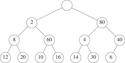
Figure 8.5The SMMH of Figure 8.4 with 2 inserted.
Let us now insert 50 into the SMMH of Figure 8.5. Since an SMMH is a complete binary tree, the new node must be positioned as in Figure 8.6.
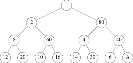
Figure 8.6The SMMH of Figure 8.5 with a node added.
Since A has a right child of its parent, we first check P1 at node A. If the new element (in this case 50) is smaller than that in the left sibling of A, we swap the new element and the element in the left sibling. In our case, no swap is done. Then we check P2 and P3. We see that placing 50 into A would violate P3. So the element 40 in the right child of the grandparent of A is moved down to node A. Figure 8.7 shows the resulting configuration. Placing 50 into node A of Figure 8.7 cannot create a P1 violation because the previous occupant of node A was smaller. Also, a P2 violation isn’t possible either. So only P3 needs to be checked at A. Since there is no P3 violation at A, 50 is placed into A.
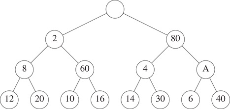
Figure 8.7The SMMH of Figure 8.6 with 40 moved down.
The algorithm to remove either the min or max element is a similar adaptation of the trickle-down algorithm used to remove an element from a min or max heap.
The twin heaps of [7], the min-max pair heaps of [6], the interval heaps of [5,8], and the diamond deques of [4] are virtually identical data structures. In each of these structures, an n element DEPQ is represented by a min heap with ⌈n/2⌉ elements and a max heap with the remaining ⌊n/2⌋ elements. The two heaps satisfy the property that each element in the min heap is ≤ the corresponding element (two elements correspond if they occupy the same position in their respective binary trees) in the max heap. When the number of elements in the DEPQ is odd, the min heap has one element (i.e., element ⌈n/2⌉) that has no corresponding element in the max heap. In the twin heaps of [7], this is handled as a special case and one element is kept outside of the two heaps. In min-max pair heaps, interval heaps, and diamond deques, the case when n is odd is handled by requiring element ⌈n/2⌉ of the min heap to be ≤ element ⌊n/4⌋ of the max heap.
In the twin heaps of [7], the min and max heaps are stored in two arrays min and max using the standard array representation of a complete binary tree* [9]. The correspondence property becomes min[i] ≤ max[i], 1 ≤ i ≤ ⌊n/2⌋. In the min-max pair heaps of [6] and the interval heaps of [5], the two heaps are stored in a single array minmax and we have minmax[i].min being the i’th element of the min heap, 1 ≤ i ≤ ⌈n/2⌉ and minmax[i].max being the i’th element of the max heap, 1 ≤ i ≤ ⌊n/2⌋. In the diamond deque [4], the two heaps are mapped into a single array with the min heap occupying even positions (beginning with position 0) and the max heap occupying odd positions (beginning with position 1). Since this mapping is slightly more complex than the ones used in twin heaps, min-max pair heaps, and interval heaps, actual implementations of the diamond deque are expected to be slightly slower than implementations of the remaining three structures.
Since the twin heaps of [7], the min-max pair heaps of [6], the interval heaps of [5], and the diamond deques of [4] are virtually identical data structures, we describe only one of these—interval heaps—in detail. An interval heap is a complete binary tree in which each node, except possibly the last one (the nodes of the complete binary tree are ordered using a level order traversal), contains two elements. Let the two elements in node P be a and b, where a ≤ b. We say that the node P represents the closed interval [a, b]. a is the left end point of the interval of P, and b is its right end point.
The interval [c, d] is contained in the interval [a, b] iff a ≤ c ≤ d ≤ b. In an interval heap, the intervals represented by the left and right children (if they exist) of each node P are contained in the interval represented by P. When the last node contains a single element c, then a ≤ c ≤ b, where [a, b] is the interval of the parent (if any) of the last node.
Figure 8.8 shows an interval heap with 26 elements. You may verify that the intervals represented by the children of any node P are contained in the interval of P.
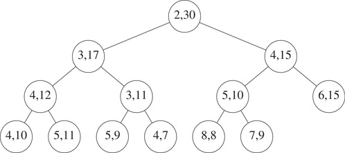
Figure 8.8An interval heap.
The following facts are immediate:
1.The left end points of the node intervals define a min heap, and the right end points define a max heap. In case the number of elements is odd, the last node has a single element which may be regarded as a member of either the min or max heap. Figure 8.9 shows the min and max heaps defined by the interval heap of Figure 8.8.
2.When the root has two elements, the left end point of the root is the minimum element in the interval heap and the right end point is the maximum. When the root has only one element, the interval heap contains just one element. This element is both the minimum and maximum element.
3.An interval heap can be represented compactly by mapping into an array as is done for ordinary heaps. However, now, each array position must have space for two elements.
4.The height of an interval heap with n elements is Θ(log n).
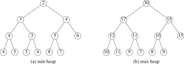
Figure 8.9Min and max heaps embedded in Figure 8.8.
Suppose we are to insert an element into the interval heap of Figure 8.8. Since this heap currently has an even number of elements, the heap following the insertion will have an additional node A as is shown in Figure 8.10.
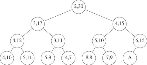
Figure 8.10Interval heap of Figure 8.8 after one node is added.
The interval for the parent of the new node A is [6, 15]. Therefore, if the new element is between 6 and 15, the new element may be inserted into node A. When the new element is less than the left end point 6 of the parent interval, the new element is inserted into the min heap embedded in the interval heap. This insertion is done using the min heap insertion procedure starting at node A. When the new element is greater than the right end point 15 of the parent interval, the new element is inserted into the max heap embedded in the interval heap. This insertion is done using the max heap insertion procedure starting at node A.
If we are to insert the element 10 into the interval heap of Figure 8.8, this element is put into the node A shown in Figure 8.10. To insert the element 3, we follow a path from node A towards the root, moving left end points down until we either pass the root or reach a node whose left end point is ≤ 3. The new element is inserted into the node that now has no left end point. Figure 8.11 shows the resulting interval heap.

Figure 8.11The interval heap of Figure 8.8 with 3 inserted.
To insert the element 40 into the interval heap of Figure 8.8, we follow a path from node A (see Figure 8.10) towards the root, moving right end points down until we either pass the root or reach a node whose right end point is ≥ 40. The new element is inserted into the node that now has no right end point. Figure 8.12 shows the resulting interval heap.
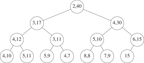
Figure 8.12The interval heap of Figure 8.8 with 40 inserted.
Now, suppose we wish to insert an element into the interval heap of Figure 8.12. Since this interval heap has an odd number of elements, the insertion of the new element does not increase the number of nodes. The insertion procedure is the same as for the case when we initially have an even number of elements. Let A denote the last node in the heap. If the new element lies within the interval [6, 15] of the parent of A, then the new element is inserted into node A (the new element becomes the left end point of A if it is less than the element currently in A). If the new element is less than the left end point 6 of the parent of A, then the new element is inserted into the embedded min heap; otherwise, the new element is inserted into the embedded max heap. Figure 8.13 shows the result of inserting the element 32 into the interval heap of Figure 8.12.
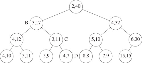
Figure 8.13The interval heap of Figure 8.12 with 32 inserted.
The removal of the minimum element is handled as several cases:
1.When the interval heap is empty, the removeMin operation fails.
2.When the interval heap has only one element, this element is the element to be returned. We leave behind an empty interval heap.
3.When there is more than one element, the left end point of the root is to be returned. This point is removed from the root. If the root is the last node of the interval heap, nothing more is to be done. When the last node is not the root node, we remove the left point p from the last node. If this causes the last node to become empty, the last node is no longer part of the heap. The point p removed from the last node is reinserted into the embedded min heap by beginning at the root. As we move down, it may be necessary to swap the current p with the right end point r of the node being examined to ensure that p ≤ r. The reinsertion is done using the same strategy as used to reinsert into an ordinary heap.
Let us remove the minimum element from the interval heap of Figure 8.13. First, the element 2 is removed from the root. Next, the left end point 15 is removed from the last node and we begin the reinsertion procedure at the root. The smaller of the min heap elements that are the children of the root is 3. Since this element is smaller than 15, we move the 3 into the root (the 3 becomes the left end point of the root) and position ourselves at the left child B of the root. Since, 15 ≤ 17 we do not swap the right end point of B with the current p = 15. The smaller of the left end points of the children of B is 3. The 3 is moved from node C into node B as its left end point and we position ourselves at node C. Since p = 15 > 11, we swap the two and 15 becomes the right end point of node C. The smaller of left end points of Cs children is 4. Since this is smaller than the current p = 11, it is moved into node C as this node’s left end point. We now position ourselves at node D. First, we swap p = 11 and Ds right end point. Now, since D has no children, the current p = 7 is inserted into node D as Ds left end point. Figure 8.14 shows the result.
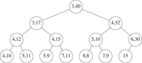
Figure 8.14The interval heap of Figure 8.13 with minimum element removed.
The max element may removed using an analogous procedure.
8.3.3Initializing an Interval Heap
Interval heaps may be initialized using a strategy similar to that used to initialize ordinary heaps–work your way from the heap bottom to the root ensuring that each subtree is an interval heap. For each subtree, first order the elements in the root; then reinsert the left end point of this subtree’s root using the reinsertion strategy used for the removeMin operation, then reinsert the right end point of this subtree’s root using the strategy used for the removeMax operation.
8.3.4Complexity of Interval Heap Operations
The operations isEmpty(), size(), getMin(), and getMax() take O(1) time each; put(x), removeMin(), and removeMax() take O(log n) each; and initializing an n element interval heap takes O(n) time.
8.3.5The Complementary Range Search Problem
In the complementary range search problem, we have a dynamic collection (i.e., points are added and removed from the collection as time goes on) of one-dimensional points (i.e., points have only an x-coordinate associated with them) and we are to answer queries of the form: what are the points outside of the interval [a, b]? For example, if the point collection is 3, 4, 5, 6, 8, 12, the points outside the range [5, 7] are 3, 4, 8, 12.
When an interval heap is used to represent the point collection, a new point can be inserted or an old one removed in O(log n) time, where n is the number of points in the collection. Note that given the location of an arbitrary element in an interval heap, this element can be removed from the interval heap in O(log n) time using an algorithm similar to that used to remove an arbitrary element from a heap.
The complementary range query can be answered in Θ(k) time, where k is the number of points outside the range [a, b]. This is done using the following recursive procedure:
1.If the interval tree is empty, return.
2.If the root interval is contained in [a, b], then all points are in the range (therefore, there are no points to report), return.
3.Report the end points of the root interval that are not in the range [a, b].
4.Recursively search the left subtree of the root for additional points that are not in the range [a, b].
5.Recursively search the right subtree of the root for additional points that are not in the range [a, b].
6.return
Let us try this procedure on the interval heap of Figure 8.13. The query interval is [4,32]. We start at the root. Since the root interval is not contained in the query interval, we reach step 3 of the procedure. Whenever step 3 is reached, we are assured that at least one of the end points of the root interval is outside the query interval. Therefore, each time step 3 is reached, at least one point is reported. In our example, both points 2 and 40 are outside the query interval and so are reported. We then search the left and right subtrees of the root for additional points. When the left subtree is searched, we again determine that the root interval is not contained in the query interval. This time only one of the root interval points (i.e., 3) is to be outside the query range. This point is reported and we proceed to search the left and right subtrees of B for additional points outside the query range. Since the interval of the left child of B is contained in the query range, the left subtree of B contains no points outside the query range. We do not explore the left subtree of B further. When the right subtree of B is searched, we report the left end point 3 of node C and proceed to search the left and right subtrees of C. Since the intervals of the roots of each of these subtrees is contained in the query interval, these subtrees are not explored further. Finally, we examine the root of the right subtree of the overall tree root, that is the node with interval [4, 32]. Since this node’s interval is contained in the query interval, the right subtree of the overall tree is not searched further.
The complexity of the above six step procedure is Θ(number of interval heap nodes visited). The nodes visited in the preceding example are the root and its two children, node B and its two children, and node C and its two children. Thus, 7 nodes are visited and a total of 4 points are reported.
We show that the total number of interval heap nodes visited is at most 3k + 1, where k is the number of points reported. If a visited node reports one or two points, give the node a count of one. If a visited node reports no points, give it a count of zero and add one to the count of its parent (unless the node is the root and so has no parent). The number of nodes with a nonzero count is at most k. Since no node has a count more than 3, the sum of the counts is at most 3k. Accounting for the possibility that the root reports no point, we see that the number of nodes visited is at most 3k + 1. Therefore, the complexity of the search is Θ(k). This complexity is asymptotically optimal because every algorithm that reports k points must spend at least Θ(1) time per reported point.
In our example search, the root gets a count of 2 (1 because it is visited and reports at least one point and another 1 because its right child is visited but reports no point), node B gets a count of 2 (1 because it is visited and reports at least one point and another 1 because its left child is visited but reports no point), and node C gets a count of 3 (1 because it is visited and reports at least one point and another 2 because its left and right children are visited and neither reports a point). The count for each of the remaining nodes in the interval heap is 0.
In the min-max heap structure [2], all n DEPQ elements are stored in an n-node complete binary tree with alternating levels being min levels and max levels (Figure 8.15, nodes at max levels are shaded). The root level of a min-max heap is a min level. Nodes on a min level are called min nodes while those on a max level are max nodes. Every min (max) node has the property that its value is the smallest (largest) value in the subtree of which it is the root. Since 5 is in a min node of Figure 8.15, it is the smallest value in its subtree. Also, since 30 and 26 are in max nodes, these are the largest values in the subtrees of which they are the root.
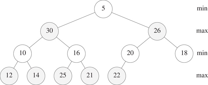
Figure 8.15A 12-element min-max heap.
The following observations are a direct consequence of the definition of a min-max heap.
1.When n = 0, there is no min nor max element.
2.When n = 1, the element in the root is both the min and the max element.
3.When n > 1, the element in the root is the min element; the max element is one of the up to two children of the root.
From these observations, it follows that getMin() and getMax() can be done in O(1) time each.
When inserting an element newElement into a min-max heap that has n elements, we go from a complete binary tree that has n nodes to one that has n + 1 nodes. So, for example, an insertion into the 12-element min-max heap of Figure 8.15 results in the 13-node complete binary tree of Figure 8.16.
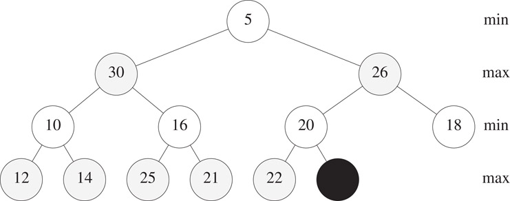
Figure 8.16A 13-node complete binary tree.
When n = 0, the insertion simply creates a min-max heap that has a single node that contains the new element. Assume that n > 0 and let the element in the parent, parentNode, of the new node j be parentElement. If newElement is placed in the new node j, the min- and max-node property can be violated only for nodes on the path from the root to parentNode. So, the insertion of an element need only be concerned with ensuring that nodes on this path satisfy the required min- and max-node property. There are three cases to consider.
1.parentElement = newElement
In this case, we may place newElement into node j. With such a placement, the min- and max-node properties of all nodes on the path from the root to parentNode are satisfied.
2.parentNode > newElement
If parentNode is a min node, we get a min-node violation. When a min-node violation occurs, we know that all max nodes on the path from the root to parentNode are greater than newElement. So, a min-node violation may be fixed by using the trickle-up process used to insert into a min heap; this trickle-up process involves only the min nodes on the path from the root to parentNode. For example, suppose that we are to insert newElement = 2 into the min-max heap of Figure 8.15. The min nodes on the path from the root to parentNode have values 5 and 20. The 20 and the 5 move down on the path and the 2 trickles up to the root node. Figure 8.17 shows the result. When newElement = 15, only the 20 moves down and the sequence of min nodes on the path from the root to j have values 5, 15, 20.
The case when parentNode is a max node is similar.
3.parentNode < newElement
When parentNode is a min node, we conclude that all min nodes on the path from the root to parentNode are smaller than newElement. So, we need be concerned only with the max nodes (if any) on the path from the root to parentNode. A trickle-up process is used to correctly position newElement with respect to the elements in the max nodes of this path. For the example of Figure 8.16, there is only one max node on the path to parentNode. This max node has the element 26. If newElement > 26, the 26 moves down to j and newElement trickles up to the former position of 26 (Figure 8.18 shows the case when newElement = 32). If newElement < 26, newElement is placed in j.
The case when parentNode is a max node is similar.
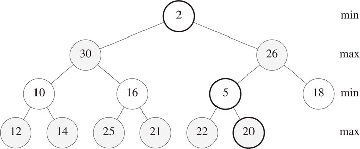
Figure 8.17Min-max heap of Figure 8.15 following insertion of 2.
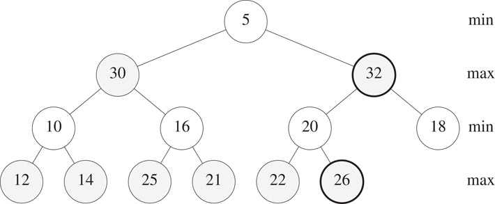
Figure 8.18The min-max heap of Figure 8.15 following the insertion of 32.
Since the height of a min-max heap is Θ(log n) and a trickle-up examines a single element at at most every other level of the min-max heap, an insert can be done in O(log n) time.
When n = 0, there is no min element to remove. When n = 1, the min-max heap becomes empty following the removal of the min element, which is in the root. So assume that n > 1. Following the removal of the min element, which is in the root, we need to go from an n-element complete binary tree to an (n − 1)-element complete binary tree. This causes the element in position n of the min-max heap array to drop out of the min-max heap. Figure 8.17 shows the situation following the removal of the min element, 5, from the min-max heap of Figure 8.15. In addition to the 5, which was the min element and which has been removed from the min-max heap, the 22 that was in position n = 12 of the min-max heap array has dropped out of the min-max heap. To get the dropped-out element 22 back into the min-max heap, we perform a trickle-down operation that begins at the root of the min-max heap.
The trickle-down operation for min-max heaps is similar to that for min and max heaps. The root is to contain the smallest element. To ensure this, we determine the smallest element in a child or grandchild of the root. If 22 is ≤ the smallest of these children and grandchildren, the 22 is placed in the root. If not, the smallest of the children and grandchildren is moved to the root; the trickle-down process is continued from the position vacated by the just moved smallest element.
In our example, examining the children and grandchildren of the root of Figure 8.19, we determine that the smallest of these is 10. Since 10 < 22, the 10 moves to the root and the 22 trickles down (Figure 8.20). A special case arises when this trickle down of the 22 by 2 levels causes the 22 to trickle past a smaller element (in our example, we trickle past a larger element 30). When this special case arises, we simply exchange the 22 and the smaller element being trickled past. The trickle-down process applied at the vacant node of Figure 8.20 results in the 22 being placed into the vacant node.
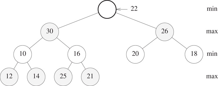
Figure 8.19Situation following a remove min from Figure 8.15.
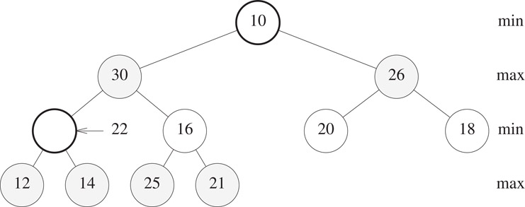
Figure 8.20Situation following one iteration of the trickle-down process.
Suppose that droppedElement is the element dropped from minmaxHeap[n] when a remove min is done from an n-element min-max heap. The following describes the trickle-down process used to reinsert the dropped element.
1.The root has no children.
In this case droppedElement is inserted into the root and the trickle down terminates.
2.The root has at least one child.
Now the smallest key in the min-max heap is in one of the children or grandchildren of the root. We determine which of these nodes has the smallest key. Let this be node k. The following possibilities need to be considered:
a.droppedElement ≤ minmaxHeap[k].
droppedElement may be inserted into the root, as there is no smaller element in the heap. The trickle down terminates.
c.droppedElement > minmaxHeap[k] and k is a child of the root.
Since k is a max node, it has no descendants larger than minmaxHeap[k]. Hence, node k has no descendants larger than droppedElement. So, the minmaxHeap[k] may be moved to the root, and droppedElement placed into node k. The trickle down terminates.
e.droppedElement > minmaxHeap[k] and k is a grandchild of the root.
minmaxHeap[k] is moved to the root. Let p be the parent of k. If droppedElement > minmaxHeap[p], then minmaxHeap[p] and droppedElement are interchanged. This interchange ensures that the max node p contains the largest key in the subheap with root p. The trickle down continues with k as the root of a min-max (sub) heap into which an element is to be inserted.
The complexity of the remove-min operation is readily seen to be O(log n). The remove-max operation is similar to the remove-min operation, and min-max heaps may be initialized in Θ(n) time using an algorithm similar to that used to initialize min and max heaps [9].
The deap structure of [3] is similar to the two-heap structures of [4–7]. At the conceptual level, we have a min heap and a max heap. However, the distribution of elements between the two is not ⌈n/2⌉ and ⌊n/2⌋. Rather, we begin with an (n + 1)-node complete binary tree. Its left subtree is the min heap and its right subtree is the max heap (Figure 8.21, max-heap nodes are shaded). The correspondence property for deaps is slightly more complex than that for the two-heap structures of [4–7].
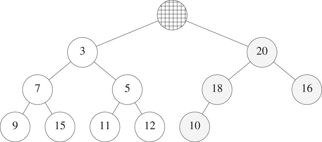
Figure 8.21An 11-element deap.
A deap is a complete binary tree that is either empty or satisfies the following conditions:
1.The root is empty.
2.The left subtree is a min heap and the right subtree is a max heap.
3.Correspondence property. Suppose that the right subtree is not empty. For every node x in the left subtree, define its corresponding node y in the right subtree to be the node in the same position as x. In case such a y doesn’t exist, let y be the corresponding node for the parent of x. The element in x is ≤ the element in y.
For the example complete binary tree of Figure 8.21, the corresponding nodes for the nodes with 3, 7, 5, 9, 15, 11, and 12, respectively, have 20, 18, 16, 10, 18, 16, and 16.
Notice that every node y in the max heap has a unique corresponding node x in the min heap. The correspondence property for max-heap nodes is that the element in y be ≥ the element in x. When the correspondence property is satisfied for all nodes in the min heap, this property is also satisfied for all nodes in the max heap.
We see that when n = 0, there is no min or max element, when n = 1, the root of the min heap has both the min and the max element, and when n > 1, the root of the min heap is the min element and the root of the max heap is the max element. So, both getMin() and getMax() may be implemented to work in O(1) time.
When an element is inserted into an n-element deap, we go form a complete binary tree that has n + 1 nodes to one that has n + 2 nodes. So, the shape of the new deap is well defined. Following an insertion, our 11-element deap of Figure 8.21 has the shape shown in Figure 8.22. The new node is node j and its corresponding node is node i.
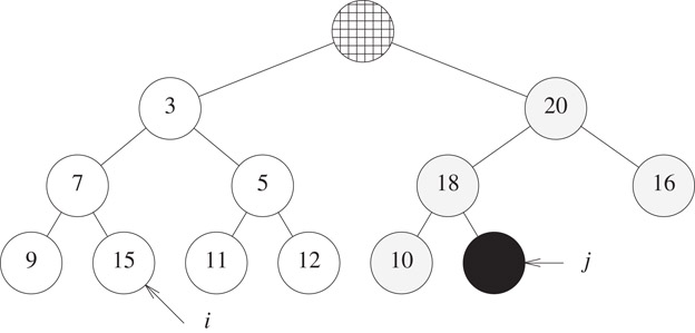
Figure 8.22Shape of a 12-element deap.
To insert newElement, temporarily place newElement into the new node j and check the correspondence property for node j. If the property isn’t satisfied, swap newElement and the element in its corresponding node; use a trickle-up process to correctly position newElement in the heap for the corresponding node i. If the correspondence property is satisfied, do not swap newElement; instead use a trickle-up process to correctly place newElement in the heap that contains node j.
Consider the insertion of newElement = 2 into Figure 8.22. The element in the corresponding node i is 15. Since the correspondence property isn’t satisfied, we swap 2 and 15. Node j now contains 15 and this swap is guaranteed to preserve the max-heap properties of the right subtree of the complete binary tree. To correctly position the 2 in the left subtree, we use the standard min-heap trickle-up process beginning at node i. This results in the configuration of Figure 8.23.
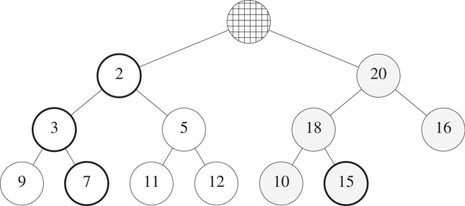
Figure 8.23Deap of Figure 8.21 with 2 inserted.
To insert newElement = 19 into the deap of Figure 8.22, we check the correspondence property between 15 and 19. The property is satisfied. So, we use the trickle-up process for max heaps to correctly position newElement in the max heap. Figure 8.24 shows the result.
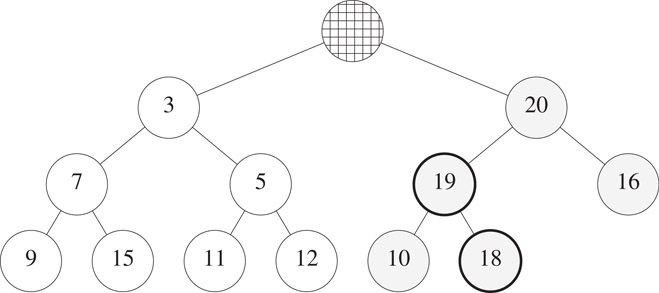
Figure 8.24Deap of Figure 8.21 with 19 inserted.
Since the height of a deap is Θ(log n), the time to insert into a deap is O(log n).
Assume that n > 0. The min element is in the root of the min heap. Following its removal, the deap size reduces to n − 1 and the element in position n + 1 of the deap array is dropped from the deap. In the case of our example of Figure 8.21, the min element 3 is removed and the 10 is dropped. To reinsert the dropped element, we first trickle the vacancy in the root of the min heap down to a leaf of the min heap. This is similar to a standard min-heap trickle down with ∞ as the reinsert element. For our example, this trickle down causes 5 and 11 to, respectively, move to their parent nodes. Then, the dropped element 10 is inserted using a trickle-up process beginning at the vacant leaf of the min heap. The resulting deap is shown in Figure 8.25.
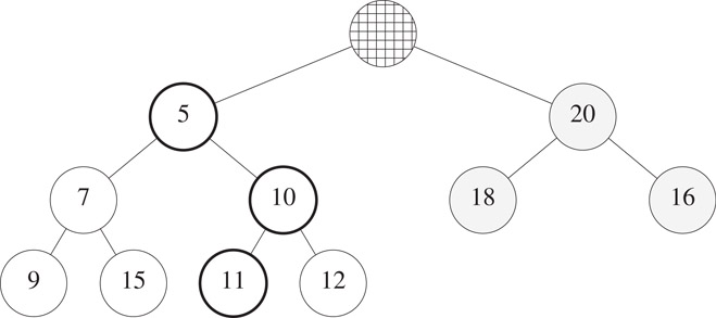
Figure 8.25Deap of Figure 8.21 following a remove min operation.
Since a removeMin requires a trickle-down pass followed by a trickle-up pass and since the height of a deap is Θ(log n), the time for a removeMin is O(log n). A removeMax is similar. Also, we may initialize a deap in Θ(n) time using an algorithm similar to that used to initialize a min or max heap [9].
General methods [10] exist to arrive at efficient DEPQ data structures from single-ended priority queue data structures that also provide an efficient implementation of the remove (theNode) operation (this operation removes the node theNode from the PQ). The simplest of these methods, dual structure method, maintains both a min PQ (called minPQ) and a max PQ (called maxPQ) of all the DEPQ elements together with correspondence pointers between the nodes of the min PQ and the max PQ that contain the same element. Figure 8.26 shows a dual heap structure for the elements 6, 7, 2, 5, 4. Correspondence pointers are shown as double-headed arrows.
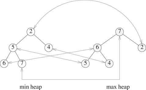
Figure 8.26Dual heap.
Although Figure 8.26 shows each element stored in both the min and the max heap, it is necessary to store each element in only one of the two heaps.
The minimum element is at the root of the min heap and the maximum element is at the root of the max heap. To insert an element x, we insert x into both the min and the max heaps and then set up correspondence pointers between the locations of x in the min and max heaps. To remove the minimum element, we do a removeMin from the min heap and a remove(theNode), where theNode is the corresponding node for the removed element, from the max heap. The maximum element is removed in an analogous way.
The notion of total correspondence borrows heavily from the ideas used in a twin heap [7]. In the twin heap data structure n elements are stored in a min heap using an array minHeap[1:n] and n other elements are stored in a max heap using the array maxHeap[1 : n]. The min and max heaps satisfy the inequality minHeap[i] ≤ maxHeap[i], 1 ≤ i ≤ n. In this way, we can represent a DEPQ with 2n elements. When we must represent a DEPQ with an odd number of elements, one element is stored in a buffer, and the remaining elements are divided equally between the arrays minHeap and maxHeap.
In total correspondence, we remove the positional requirement in the relationship between pairs of elements in the min heap and max heap. The requirement becomes: for each element a in minPQ there is a distinct element b in maxPQ such that a ≤ b and vice versa. (a, b) is a corresponding pair of elements. Figure 8.27a shows a twin heap with 11 elements and Figure 8.27b shows a total correspondence heap. The broken arrows connect corresponding pairs of elements.
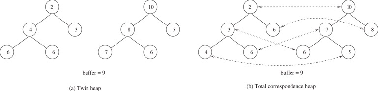
Figure 8.27Twin heap and total correspondence heap.
In a twin heap the corresponding pairs (minHeap[i], maxHeap[i]) are implicit, whereas in a total correspondence heap these pairs are represented using explicit pointers.
In a total correspondence DEPQ, the number of nodes is either n or n − 1. The space requirement is half that needed by the dual priority queue representation. The time required is also reduced. For example, if we do a sequence of inserts, every other one simply puts the element in the buffer. The remaining inserts put one element in maxPQ and one in minPQ. So, on average, an insert takes time comparable to an insert in either maxPQ or minPQ. Recall that when dual priority queues are used the insert time is the sum of the times to insert into maxPQ and minPQ. Note also that the size of maxPQ and minPQ together is half that of a dual priority queue.
If we assume that the complexity of the insert operation for priority queues as well as 2 remove(theNode) operations is no more than that of the delete max or min operation (this is true for all known priority queue structures other than weight biased leftist trees [11]), then the complexity of removeMax and removeMin for total correspondence DEPQs is the same as for the removeMax and removeMin operation of the underlying priority queue data structure.
Using the notion of total correspondence, we trivially obtain efficient DEPQ structures starting with any of the known priority queue structures (other than weight biased leftist trees [11]).
The removeMax and removeMin operations can generally be programmed to run faster than suggested by our generic algorithms. This is because, for example, a removeMax() and put(x) into a max priority queue can often be done faster as a single operation changeMax(x). Similarly a remove(theNode) and put(x) can be programmed as a change (theNode, x) operation.
In leaf correspondence DEPQs, for every leaf element a in minPQ, there is a distinct element b in maxPQ such that a ≤ b and for every leaf element c in maxPQ there is a distinct element d in minPQ such that d ≤ c. Figure 8.28 shows a leaf correspondence heap.
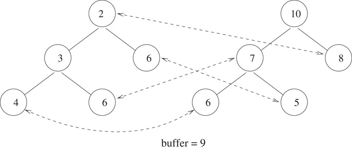
Figure 8.28Leaf correspondence heap.
Efficient leaf correspondence DEPQs may be constructed easily from PQs that satisfy the following requirements [10]:
a.The PQ supports the operation remove(Q, p) efficiently.
b.When an element is inserted into the PQ, no nonleaf node becomes a leaf node (except possibly the node for the newly inserted item).
c.When an element is deleted (using remove, removeMax or removeMin) from the PQ, no nonleaf node (except possibly the parent of the deleted node) becomes a leaf node.
Some of the PQ structures that satisfy these requirements are height-biased leftist trees (Chapter 5) [9,12, 13], pairing heaps (Chapter 7) [14,15], and Fibonacci heaps [16] (Chapter 7). Requirements (b) and (c) are not satisfied, for example, by ordinary heaps and the FMPQ structure of [17]. Although heaps and Brodal’s FMPQ structure do not satisfy the requirements of our generic approach to build a leaf correspondence DEPQ structure from a priority queue, we can nonetheless arrive at leaf correspondence heaps and leaf correspondence FMPQs using a customized approach.
A meldable DEPQ (MDEPQ) is a DEPQ that, in addition to the DEPQ operations listed above, includes the operation
The result of melding the double-ended priority queues x and y is a single double-ended priority queue that contains all elements of x and y. The meld operation is destructive in that following the meld, x and y do not remain as independent DEPQs.
To meld two DEPQs in less than linear time, it is essential that the DEPQs be represented using explicit pointers (rather than implicit ones as in the array representation of a heap) as otherwise a linear number of elements need to be moved from their initial to their final locations. Olariu et al. [6] have shown that when the min-max pair heap is represented in such a way, an n element DEPQ may be melded with a k element one (k ≤ n) in O(log (n/k) * log k) time. When , this is O(log2n). Hasham and Sack [18] have shown that the complexity of melding two min-max heaps of size n and k, respectively, is Ω(n + k). Brodal [17] has developed an MDEPQ implementation that allows one to find the min and max elements, insert an element, and meld two priority queues in O(1) time. The time needed to delete the minimum or maximum element is O(log n). Although the asymptotic complexity provided by this data structure are the best one can hope for [17], the data structure has practical limitations. First, each element is represented twice using a total of 16 fields per element. Second, even though the delete operations have O(log n) complexity, the constant factors are very high and the data structure will not perform well unless find, insert, and meld are the primary operations.
Cho and Sahni [19] have shown that leftist trees [9, 12, 13] may be adapted to obtain a simple representation for MDEPQs in which meld takes logarithmic time and the remaining operations have the same asymptotic complexity as when any of the aforementioned DEPQ representations is used. Chong and Sahni [10] study MDEPQs based on pairing heaps [14, 15], Binomial and Fibonacci heaps [16], and FMPQ [17].
Since leftist heaps, pairing heaps, Binomial and Fibonacci heaps, and FMPQs are meldable priority queues that also support the remove(theNode) operation, the MDEPQs of [10, 19] use the generic methods of Section 8.6 to construct an MDEPQ data structure from the corresponding MPQ (meldable PQ) structure.
It is interesting to note that if we use the FMPQ structure of [17] as the base MPQ structure, we obtain a total correspondence MDEPQ structure in which removeMax and removeMin take logarithmic time, and the remaining operations take constant time. This adaptation is superior to the dual priority queue adaptation proposed in Reference 17 because the space requirements are almost half. Additionally, the total correspondence adaptation is faster. Although Brodal’s FMPQ structure does not satisfy the requirements of the generic approach to build a leaf correspondence MDEPQ structure from a priority queue, we can nonetheless arrive at leaf correspondence FMPQs using a customized approach.
This work was supported, in part, by the National Science Foundation under grant CCR-9912395.
1.A. Arvind and C. Pandu Rangan, Symmetric min-max heap: A simpler data structure for double-ended priority queue, Information Processing Letters, 69, 197–199, 1999.
2.M. Atkinson, J. Sack, N. Santoro, and T. Strothotte, Min-max heaps and generalized priority queues, Communications of the ACM, 29, 996–1000, 1986.
3.S. Carlsson, The deap—A double ended heap to implement double ended priority queues, Information Processing Letters, 26, 33–36, 1987.
4.S. Chang and M. Du, Diamond deque: A simple data structure for priority deques, Information Processing Letters, 46, 231–237, 1993.
5.J. van Leeuwen and D. Wood, Interval heaps, The Computer Journal, 36, 3, 209–216, 1993.
6.S. Olariu, C. Overstreet, and Z. Wen, A mergeable double-ended priority queue, The Computer Journal, 34 5, 423–427, 1991.
7.J. Williams, Algorithm 232, Communications of the ACM, 7, 347–348, 1964.
8.Y. Ding and M. Weiss, On the complexity of building an interval heap, Information Processing Letters, 50, 143–144, 1994.
9.E. Horowitz, S. Sahni, and D. Mehta, Fundamentals of Data Structures in C++, Computer Science Press, NY, 1995.
10.K. Chong and S. Sahni, Correspondence based data structures for double ended priority queues, ACM Journal on Experimental Algorithmics, 5, Article 2, 22, 2000.
11.S. Cho and S. Sahni, Weight biased leftist trees and modified skip lists, ACM Journal on Experimental Algorithms, Article 2, 1998.
12.C. Crane, Linear lists and priority queues as balanced binary trees, Technical Report CS-72-259, Computer Science Department, Stanford University, Standford, CA, 1972.
13.R. Tarjan, Data Structures and Network Algorithms, SIAM, Philadelphia, PA, 1983.
14.M. L. Fredman, R. Sedgewick, D. D. Sleator, and R. E. Tarjan, The paring heap: A new form of self-adjusting heap, Algorithmica, 1, 111–129, 1986.
15.J. T. Stasko and J. S. Vitter, Pairing heaps: Experiments and analysis, Communication of the ACM, 30, 3, 234–249, 1987.
16.M. Fredman and R. Tarjan, Fibonacci heaps and their uses in improved network optimization algorithms, JACM, 34, 3, 596–615, 1987.
17.G. Brodal, Fast meldable priority queues, Workshop on Algorithms and Data Structures, 1995.
18.A. Hasham and J. Sack, Bounds for min-max heaps, BIT, 27, 315–323, 1987.
19.S. Cho and S. Sahni, Mergeable double ended priority queue, International Journal on Foundation of Computer Sciences, 10, 1, 1–18, 1999.
20.Y. Ding and M. Weiss, The relaxed min-max heap: A mergeable double-ended priority queue, Acta Informatica, 30, 215–231, 1993.
21.D. Sleator and R. Tarjan, Self-adjusting binary search trees, JACM, 32, 3, 652–686, 1985.
*This chapter has been reprinted from first edition of this Handbook, without any content updates.
*A minPQ supports the operations getmin(), put(x), and removeMin() while a maxPQ supports the operations getMax(), put(x), and removeMax().
*In a full binary tree, every non-empty level has the maximum number of nodes possible for that level. Number the nodes in a full binary tree 1, 2, … beginning with the root level and within a level from left to right. The nodes numbered 1 through n define the unique complete binary tree that has n nodes.