
Siu-Wing Cheng
Hong Kong University of Science and Technology
Edge Insertion and Deletion•Vertex Split and Edge Contraction
Access Functions•Edge Insertion and Deletion•Vertex Split and Edge Contraction
Graphs (Chapter 4) have found extensive applications in computer science as a modeling tool. In mathematical terms, a graph is simply a collection of vertices and edges. Indeed, a popular graph data structure is the adjacency lists representation [1] in which each vertex keeps a list of vertices connected to it by edges. In a typical application, the vertices model entities and an edge models a relation between the entities corresponding to the edge endpoints. For example, the transportation problem calls for a minimum cost shipping pattern from a set of origins to a set of destinations [2]. This can be modeled as a complete directed bipartite graph. The origins and destinations are represented by two columns of vertices. Each origin vertex is labeled with the amount of supply stored there. Each destination vertex is labeled with the amount of demand required there. The edges are directed from the origin vertices to the destination vertices and each edge is labeled with the unit cost of transportation. Only the adjacency information between vertices and edges are useful and captured, apart from the application dependent information.
In geometric computing, graphs are also useful for representing various diagrams. We restrict our attention to diagrams that are planar graphs embedded in the plane using straight edges without edge crossings. Such diagrams are called planar straight line graphs and denoted by PSLGs for short. Examples include Voronoi diagrams, arrangements, and triangulations. Their definitions can be found in standard computational geometry texts such as the book by de Berg et al. [3]. See also Chapters 65, 66, and 67. For completeness, we also provide their definitions in Section 18.8. The straight edges in a PSLG partition the plane into regions with disjoint interior. We call these regions faces. The adjacency lists representation is usually inadequate for applications that manipulate PSLGs. Consider the problem of locating the face containing a query point in a Delaunay triangulation. One practical algorithm is to walk towards the query point from a randomly chosen starting vertex [4], see Figure 18.1. To support this algorithm, one needs to know the first face that we enter as well as the next face that we step into whenever we cross an edge. Such information is not readily provided by an adjacency lists representation.
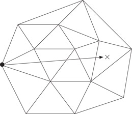
Figure 18.1Locate the face containing the cross by walking from a randomly chosen vertex.
There are three well-known data structures for representing PSLGs: the winged-edge, halfedge, and quadedge data structures. In Sections 18.2 and 18.3, we discuss the PSLGs that we deal with in more details and the operations on PSLGs. Afterwards, we introduce the three data structures in Sections 18.4 through 18.6. We conclude in Section 18.7 with some further remarks.
We assume that each face has exactly one boundary and we allow dangling edges on a face boundary. These assumptions are valid for many important classes of PSLGs such as triangulations, Voronoi diagrams, planar subdivisions with no holes, arrangements of lines, and some special arrangements of line segments (see Figure 18.2).
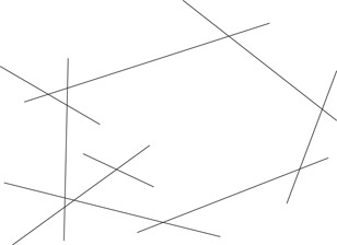
Figure 18.2Dangling edges.
There is at least one unbounded face in a PSLG but there could be more than one, for example, in the arrangement of lines shown in Figure 18.3.
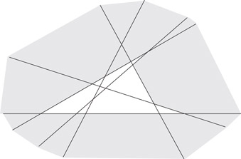
Figure 18.3The shaded faces are the unbounded faces of the arrangement.
The example also shows that there may be some infinite edges. To handle infinite edges like halflines and lines, we need a special vertex vinf at infinity. One can imagine that the PSLG is placed in a small almost flat disk D at the north pole of a giant sphere S and vinf is placed at the south pole. If an edge e is a halfline originating from a vertex u, then the endpoints of e are u and vinf. One can view e as a curve on S from u near the north pole to vinf at the south pole, but e behaves as a halfline inside the disk D. If an edge e is a line, then vinf is the only endpoint of e. One can view e as a loop from vinf to the north pole and back, but e behaves as a line inside the disk D.
We do not allow isolated vertices, except for vinf. Planarity implies that the incident edges of each vertex are circularly ordered around that vertex. This applies to vinf as well.
A PSLG data structure keeps three kinds of attributes: vertex attributes, edge attributes, and face attributes. The attributes of a vertex include its coordinates except for vinf (we assume that vinf is tagged to distinguish it from other vertices). The attributes of an edge include the equation of the support line of the edge (in the form of Ax + By + C = 0). The face attributes are useful for auxiliary information, for example, color.
The operations on a PSLG can be classified into access functions and structural operations. The access functions retrieve information without modifying the PSLG. Since the access functions partly depend on the data structure, we discuss them later when we introduce the data structures. In this section, we discuss four structural operations on PSLGs: edge insertion, edge deletion, vertex split, and edge contraction. We concentrate on the semantics of these four operations and discuss the implementation details later when we introduce the data structures. For vertex split and edge contraction, we assume further that each face in the PSLG is a simple polygon as these two operations are usually used under such circumstances.
18.3.1Edge Insertion and Deletion
When a new edge e with endpoints u and v is inserted, we assume that e does not cross any existing edge. If u or v is not an existing vertex, the vertex will be created. If both u and v are new vertices, e is an isolated edge inside a face f. Since each face is assumed to have exactly one boundary, this case happens only when the PSLG is empty and f is the entire plane. Note that e becomes a new boundary of f. If either u or v is a new vertex, then the boundary of exactly one face gains the edge e. If both u and v already exist, then u and v lie on the boundary of a face which is split into two new faces by the insertion of e. These cases are illustrated in Figure 18.4.
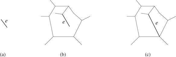
Figure 18.4Cases in edge insertion.
The deletion of an edge e has the opposite effects. After the deletion of e, if any of its endpoint becomes an isolated vertex, it will be removed. The vertex vinf is an exception and it is the only possible isolated vertex. The edge insertion is clearly needed to create a PSLG from scratch. Other effects can be achieved by combining edge insertions and deletions appropriately. For example, one can use the two operations to overlay two PSLGs in a plane sweep algorithm, see Figure 18.5.
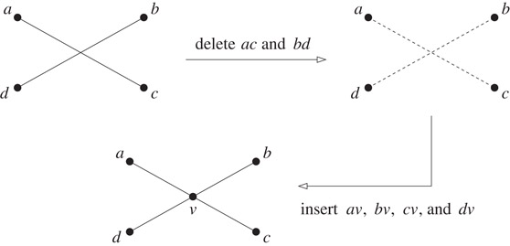
Figure 18.5Intersecting two edges.
18.3.2Vertex Split and Edge Contraction
The splitting of a vertex v is best visualized as the continuous morphing of v into an edge e. Depending on the specification of the splitting, an incident face of v gains e on its boundary or an incident edge of v is split into a triangular face, see Figure 18.6. The incident edges of v are displaced and it is assumed that no self-intersection occurs within the PSLG during the splitting. The contraction of an edge e is the inverse of the vertex split. We also assume that no self-intersection occurs during the edge contraction. If e is incident on a triangular face, that face will disappear after the contraction of e.
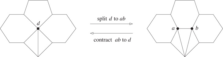
Figure 18.6Vertex split and edge contraction.
Not every edge can be contracted. Consider an edge ab. If the PSLG contains a cycle abv that is not the boundary of any face incident to ab, we call the edge ab non-contractible because its contraction is not cleanly defined. Figure 18.7 shows an example. In the figure, after the contraction, there is an ambiguity whether dv should be incident on the face f1 or the face f2. In fact, one would expect the edge dv to behave like av and bv and be incident on both f1 and f2 after the contraction. However, this is impossible.
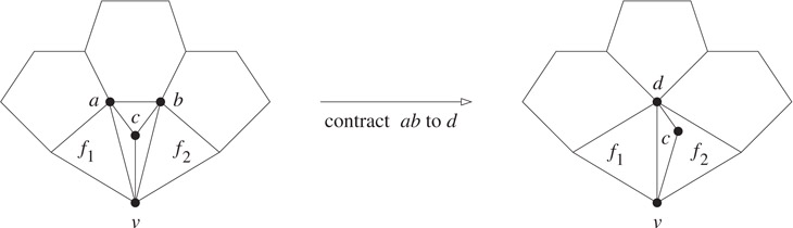
Figure 18.7Non-contractible edge.
The vertex split and edge contraction have been used in clustering and hierarchical drawing of maximal planar graphs [5].
The winged-edge data structure was introduced by Baumgart [6] and it predates the halfedge and quadedge data structures. There are three kinds of records: vertex records, edge records, and face records. Each vertex record keeps a reference to one incident edge of the vertex. Each face record keeps a reference to one boundary edge of the face. Each edge e is stored as an oriented edge with the following references (see Figure 18.8):
•The origin endpoint e.org and the destination endpoint e.dest of e. The convention is that e is directed from e.org to e.dest.
•The faces e.left and e.right on the left and right of e, respectively.
•The two edges e.lcw and e.lccw adjacent to e that bound the face e.left. The edge e.lcw is incident to e.org and the edge e.lccw is incident to e.dest. Note that e.lcw (resp. e.lccw) succeeds e if the boundary of e.left is traversed in the clockwise (resp. anti-clockwise) direction from e.
•The two edges e.rcw and e.rccw adjacent to e that bound the face e.right. The edge e.rcw is incident to e.dest and the edge e.rccw is incident to e.org. Note that e.rcw (resp. e.rccw) succeeds e if the boundary of e.right is traversed in the clockwise (resp. anti-clockwise) direction from e.
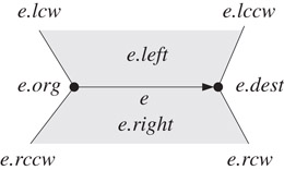
Figure 18.8Winged-edge data structure.
The information in each edge record can be retrieved in constant time. Given a vertex v, an edge e, and a face f, we can thus answer in constant time whether v is incident on e and e is incident on f. Given a vertex v, we can traverse the edges incident to v in clockwise order as follows. We output the edge e kept at the vertex record for v. We perform e := e.rccw if v = e.org and e := e.lccw otherwise. Then we output e and repeat the above. Given a face f, we can traverse its boundary edges in clockwise order as follows. We output the edge e kept at the face record for f. We perform e := e.lcw if f = e.left and e := e.rcw otherwise. Then we output e and repeat the above.
Note that an edge reference does not carry information about the orientation of the edge. Also, the orientations of the boundary edges of a face need not be consistent with either the clockwise or anti-clockwise traversal. Thus, the manipulation of the data structure is often complicated by case distinctions. We illustrate this with the insertion of an edge e. Assume that e.org = u, e.dest = v, and both u and v already exist. The input also specifies two edges e1 and e2 incident to u and v, respectively. The new edge e is supposed to immediately succeed e1 (resp. e2) in the anti-clockwise ordering of edges around u (resp. v). The insertion routine works as follows.
1.If u = vinf and it is isolated, we need to store the reference to e in the vertex record for u. We update the vertex record for v similarly.
2.Let e3 be the incident edge of u following e1 such that e is to be inserted between e1 and e3. Note that e3 succeeds e1 in anti-clockwise order. We insert e between e1 and e3 as follows.
e.rccw := e1; e.lcw := e3;
if e.org = e1.org then e1.lcw := e; else e1.rcw := e;
if e.org = e3.org then e3.rccw := e; else e3.lccw := e;
3.Let e4 be the incident edge of v following e2 such that e is to be inserted between e2 and e4. Note that e4 succeeds e2 in anti-clockwise order. We insert e between e2 and e4 as follows.
e.lccw := e2; e.rcw := e4;
if e.dest = e2.dest then e2.rcw := e; else e2.lcw := e;
if e.dest = e4.dest then e4.lccw := e; else e4.rccw := e;
4.The insertion of e has split a face into two. So we create a new face f and make e.left reference it. Also, we store a reference to e in the face record for f. There are further ramifications. First, we make e.right reference the old face.
if e.org = e1.org then e.right := e1.left; else e.right := e1.right;
Second, we make the left or right fields of the boundary edges of f reference f.
        e′ := e; w := e.org;
        repeat
           if e′.org = w then e′.left := f; w := e′.dest; e′ := e′.lccw
                         else e′.right := f; w :=e′.org; e′ := e′.rccw
        until e′ = e;
Notice the inconvenient case distinctions needed in steps 2, 3, and 4. The halfedge data structure is designed to keep both orientations of the edges and link them properly. This eliminates most of these case distinctions as well as simplifies the storage scheme.
In the halfedge data structure, for each edge in the PSLG, there are two symmetric edge records for the two possible orientations of the edge [7]. This solves the orientation problem in the winged-edge data structure. The halfedge data structure is also known as the doubly connected edge list [3]. We remark that the name doubly connected edge list was first used to denote the variant of the winged-edge data structure in which the lccw and rccw fields are omitted [8,9].
There are three kinds of records: vertex records, halfedge records, and face records. Let e be a halfedge. The following information is kept at the record for e (see Figure 18.9).
•The reference e.sym to the symmetric version of e.
•The origin endpoint e.org of e. We do not need to store the destination endpoint of e since it can be accessed as e.sym.org. The convention is that e is directed from e.org to e.sym.org.
•The face e.left on the left of e.
•The next edge e.succ and the previous edge e.pred in the anti-clockwise traversal around the face e.left.
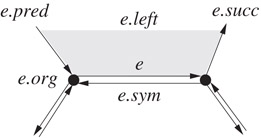
Figure 18.9Halfedge data structure.
For each vertex v, its record keeps a reference to one halfedge v.edge such that v = v.edge.org. For each face f, its record keeps a reference to one halfedge f.edge such that f = f.edge.left.
We introduce two basic operations make_halfedges and half_splice which will be needed for implementing the operations on PSLGs. These two operations are motivated by the operations make_edge and splice introduced by Guibas and Stolfi [10] for the quadedge data structure. We can also do without make_halfedges and half_splice, but they make things simpler.
•make_halfedges(u, v): Return two halfedges e and e.sym connecting the points u and v. The halfedges e and e.sym are initialized such that they represent a new PSLG with e and e.sym as the only halfedges. That is, e.succ = e.sym = e.pred and e.sym.succ = e = e.sym.pred. Also, e is the halfedge directed from u to v. If u and v are omitted, it means that the actual coordinates of e.org and e.sym.org are unimportant.
•half_splice(e1, e2): Given two halfedges e1 and e2, half_splice swaps the contents of e1.pred and e2.pred and the contents of e1.pred.succ and e2.pred.succ. The effects are:
•Let v = e2.org. If e1.org ≠ v, the incident halfedges of e1.org and e2.org are merged into one circular list (see Figure 18.10a). The vertex v is now redundant and we finish the merging as follows.
             e′ := e2;
             repeat
               e′.org := e1.org; e′ := e′.sym.succ;
             until e′ = e2;
             delete the vertex record for v;
•Let v = e2.org. If e1.org = v, the incident halfedges of v are separated into two circular lists (see Figure 18.10b). We create a new vertex u for e2.org with the coordinates of u left uninitialized. Then we finish the separation as follows.
             u.edge := e2; e′ := e2;
             repeat
               e′.org := u; e′ := e′.sym.succ;
             until e′ = e2.
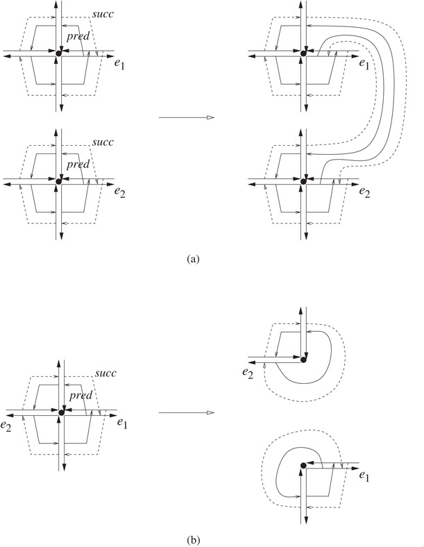
Figure 18.10The effects of half_splice.
The behavior of half_splice is somewhat complex even in the following special cases. If e is an isolated halfedge, half_splice(e1, e) deletes the vertex record for e.org and makes e a halfedge incident to e1.org following e1 in anti-clockwise order. If e1 = e.sym.succ, half_splice(e1, e) detaches e from the vertex e1.org and creates a new vertex record for e.org. If e1 = e, half_splice(e, e) has no effect at all.
The information in each halfedge record can be retrieved in constant time. Given a vertex v, a halfedge e, and a face f, we can thus answer the following adjacency queries:
1.Is v incident on e? This is done by checking if v = e.org or e.sym.org.
2.Is e incident on f? This is done by checking if f = e.left.
3.List the halfedges with origin v in clockwise order. Let e = v.edge. Output e, perform e := e.sym.succ, and then repeat until we return to v.edge.
4.List the boundary halfedges of f in anti-clockwise order. Let e = f.edge. Output e, perform e := e.succ, and then repeat until we return to f.edge.
Other adjacency queries (e.g., listing the boundary vertices of a face) can be answered similarly.
18.5.2Edge Insertion and Deletion
The edge insertion routine takes two vertices u and v and two halfedges e1 and e2. If u is a new vertex, e1 is ignored; otherwise, we assume that e1.org = u. Similarly, if v is a new vertex, e2 is ignored; otherwise, we assume that e2.org = v. The general case is that an edge connecting u and v is inserted between e1 and e1.pred.sym and between e2 and e2.pred.sym. The two new halfedges e and e.sym are returned with the convention that e is directed from u to v.
Algorithm insert(u, v, e1, e2)
1. (e, e.sym) :=make_halfedges(u, v); 2. if u is not new 3. thenhalf_splice(e1, e); 4. e.left := e1.left; 5. e.sym.left := e1.left; 6. if v is not new 7. thenhalf_splice(e2, e.sym); 8. e.left := e2.left; 9. e.sym.left := e2.left; 10. if neither u nor v is new 11. then /* A face has been split */ 12. e2.left.edge := e; 13. create a new face f ; 14. f.edge := e.sym; 15. e′:= e.sym; 16. repeat 17. e′.left := f ; 18. e′ := e′.succ; 19. until e′=e.sym; 20. return (e, e.sym);
The following deletion algorithm takes the two halfedges e and e.sym corresponding to the edge to be deleted. If the edge to be deleted borders two adjacent faces, they have to be merged after the deletion.
Algorithm delete(e, e.sym)
1. if e.left ≠ e.sym.left 2. then /* Figure 18.11a */ 3. /* the faces adjacent to e and e.sym are to be merged */ 4. delete the face record for e.sym.left; 5. e′:= e.sym; 6. repeat 7. e′.left := e.left; 8. e′ := e′.succ; 9. until e′=e.sym; 10. e.left.edge := e.succ; 11.half_splice(e.sym.succ, e); 12.half_splice(e.succ, e.sym); 13. else if e.succ=e.sym 14. then /* Figure 18.11b */ 15. e.left.edge := e.pred; 16.half_splice(e.sym.succ, e); 17. else /* Figure 18.11c */ 18. e.left.edge := e.succ; 19.half_splice(e.succ, e.sym); 20. /* e becomes an isolated edge */ 21. delete the vertex record for e.org if e.org≠vinf; 22. delete the vertex record for e.sym.org if e.sym.org≠vinf; 23. delete the halfedges e and e.sym;
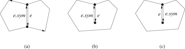
Figure 18.11Cases in deletion.
18.5.3Vertex Split and Edge Contraction
Recall that each face is assumed to be a simple polygon for the vertex split and edge contraction operations. The vertex split routine takes two points (p, q) and (x, y) and four halfedges e1, e2, e3, and e4 in anti-clockwise order around the common origin v. It is required that either e1 = e2 or e1.pred = e2.sym and either e3 = e4 or e3.pred = e4.sym. The routine splits v into an edge e connecting the points (p, q) and (x, y). Also, e borders the faces bounded by e1 and e2 and by e3 and e4. Note that if e1 = e2, we create a new face bounded by e1, e2, and e. Similarly, a new face is created if e3 = e4. The following is the vertex split algorithm.
Algorithm split(p, q, x, y, e1, e2, e3, e4)
1. if e1 ≠ e2 and e3 ≠ e4 2. then /* Figure 18.12a */ 3.half_splice(e1, e3); 4.insert(e1.org, e3.org, e1, e3); 5. set the coordinates of e3.org to (x, y); 6. set the coordinates of e1.org to (p, q); 7. else if e1 = e2 8. then a := e1.sym.succ; 9. if a≠e3 10. then /* Figure 18.12b */ 11.half_splice(a, e3); 12.insert(a.org, e3.org, a, e3); 13.insert(a.org, e1.sym.org, a, e1.sym); 14. set the coordinates of a.org to (x, y); 15. else /* Figure 18.12c */ 16. let u be a new vertex at (x, y); 17. (e, e.sym) :=insert(u, e1.org, ·, e3); 18.insert(u, e1.sym.org, e, e1.sym); 19.insert(u, e3.sym.org, e, e3.succ); 20. set the coordinates of e1.org to (p, q); 21. else b := e3.pred.sym; 22. /* since e1≠e2, b≠e2 */ 23. /* Figure 18.12d */ 24.half_splice(e1, e3); 25. (e, e.sym) :=insert(b.org, e3.org, e1, e3); 26.insert(b.org, e3.sym.org, e, e3.succ); 27. set the coordinates of b.org to (x, y); 28. set the coordinates of e3.org to (p, q);
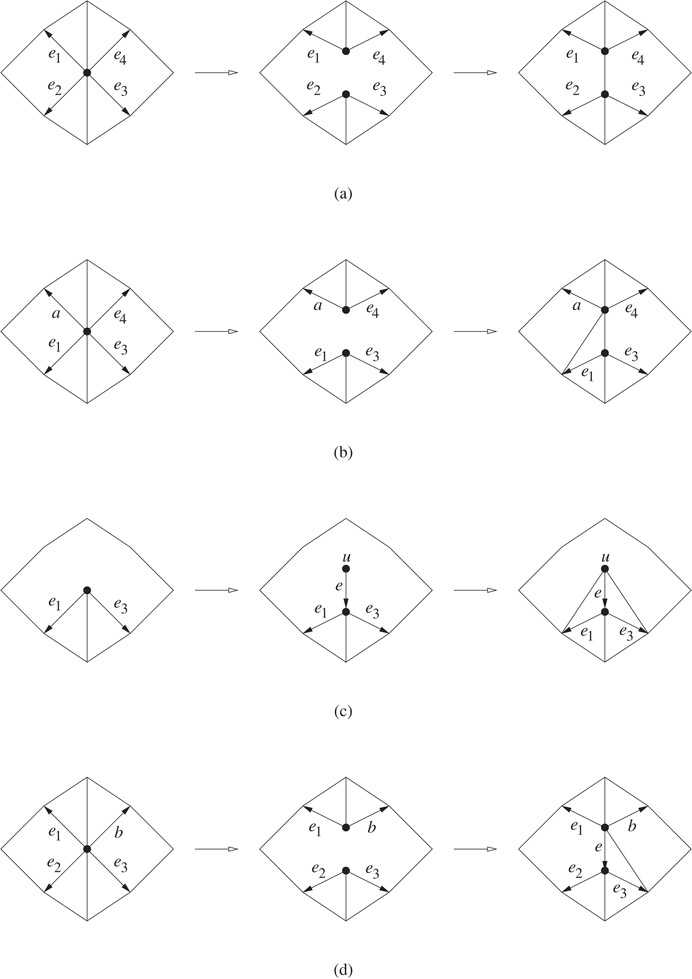
Figure 18.12Cases for split.
The following algorithm contracts an edge to a point (x, y), assuming that the edge contractibility has been checked.
Algorithm contract(e, e.sym, x, y)
1. e1 := e.succ; 2. e2 := e.pred.sym; 3. e3 := e.sym.succ; 4. e4 := e.sym.pred.sym; 5.delete(e, e.sym); 6. if e1.succ≠e2.sym and e3.succ≠e4.sym 7. then /* Figure 18.13a */ 8.half_splice(e1, e3); 9. else if e1.succ=e2.sym and e3.succ≠e4.sym 10. then /* Figure 18.13b */ 11.delete(e2, e2.sym); 12.half_splice(e1, e3); 13. else if e1.succ≠e2.sym and e3.succ=e4.sym 14. then /* symmetric to Figure 18.13b */ 15.delete(e4, e4.sym); 16.half_splice(e1, e3); 17. else /* Figure 18.13c */ 18. a := e3.sym.succ; 19.delete(e3, e3.sym); 20. if a≠e2 21. thendelete(e2, e2.sym); 22.half_splice(e1, a); 23. elsedelete(e2, e2.sym); 24. set the coordinates of e1.org to (x, y);
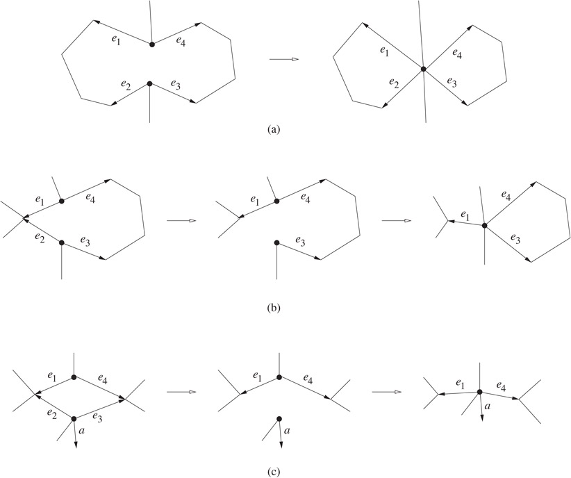
Figure 18.13Cases for contract.
The quadedge data structure was introduced by Guibas and Stolfi [10]. It represents the planar subdivision and its dual simultaneously. The dual S* of a PSLG S is constructed as follows. For each face of S, put a dual vertex inside the face. For each edge of S bordering the faces f and f′, put a dual edge connecting the dual vertices of f and f′. The dual of a vertex v in S is a face and this face is bounded by the dual of the incident edges of v. Figure 18.14 shows an example. The dual may have loops and two vertices may be connected by more than one edge, so the dual may not be a PSLG. Nevertheless, the quadedge data structure is expressive enough to represent the dual. In fact, it is powerful enough to represent subdivisions of both orientable and non-orientable surfaces. We describe a simplified version sufficient for our purposes.
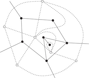
Figure 18.14The solid lines and black dots show a PSLG and the dashed lines and the white dots denote the dual.
Each edge e in the PSLG is represented by four quadedges e[i], where i ∈ {0, 1, 2, 3}. The quadedges e[0] and e[2] are the two oriented versions of e. The quadedges e[1] and e[3] are the two oriented versions of the dual of e. These four quadedges are best viewed as a cross such as e[i + 1] is obtained by rotating e[i] for π/2 in the anti-clockwise direction. This is illustrated in Figure 18.15. The quadedge e[i] has a next field referencing the quadedge that has the same origin as e[i] and follows e[i] in anti-clockwise order. In effect, the next fields form a circular linked list of quadedges with a common origin. This is called an edge ring. The following primitives are needed.
•rot(e, i): Return e[(i + 1) mod 4].
•rot−1(e, i): Return e[(i + 3) mod 4].
•sym(e, i): This function returns the quadedge with the opposite orientation of e[i]. This is done by returning rot(rot(e, i)).
•onext(e, i): Return e[i].next.
•oprev(e, i): This function gives the quadedge that has the same origin as e[i] and follows e[i] in clockwise order. This is done by returning rot(e[(i + 1) mod 4].next).
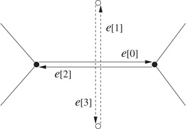
Figure 18.15Quadedges.
The quadedge data structure is entirely edge based and there are no explicit vertex and face records.
The following two basic operations make_edge and splice are central to the operations on PSLGs supported by the quadedge data structure. Our presentation is slightly different from that in the original paper [10].
•make_edge(u, v): Return an edge e connecting the points u and v. The quadedges e[i] where 0 ≤ i ≤ 3 are initialized such that they represent a new PSLG with e as the only edge. Also, e[0] is the quadedge directed from u to v. If u and v are omitted, it means that the actual coordinates of the endpoints of are unimportant.
•splice(a, i, b, j): Given two quadedges a[i] and b[j], let (c, k) = rot(a[i].next) and (d, l) = rot(b[j].next), splice swaps the contents of a[i].next and b[j].next and the contents of c[k].next and d[l].next. The effects on the edge rings of the origins of a[i] and b[j] and the edge rings of the origins of c[k] and d[l] are:
•If the two rings are different, they are merged into one (see Figure 18.16a).
•If the two rings are the same, it will be split into two separate rings (see Figure 18.16b).
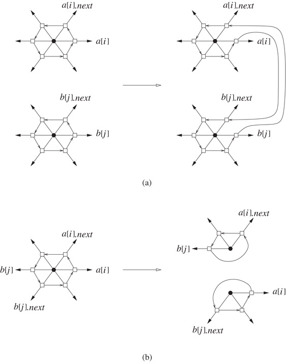
Figure 18.16The effects of splice.
Notice that make_edge and splice are similar to the operations make_halfedges and half_splice introduced for the halfedge data structure in the previous section. As mentioned before, they inspire the definitions of make_halfedges and half_splice. Due to this similarity, one can easily adapt the edge insertion, edge deletion, vertex split, and edge contraction algorithms in the previous section for the quadedge data structure.
We have assumed that each face in the PSLG has exactly one boundary. This requirement can be relaxed for the winged-edge and the halfedge data structures. One method works as follows. For each face f, pick one edge from each boundary and keep a list of references to these edges at the face record for f. Also, the edge that belongs to outer boundary of f is specially tagged. With this modification, one can traverse the boundaries of a face f consistently (e.g., keeping f on the left of traversal direction). The edge insertion and deletion algorithms also need to be enhanced. Since a face f may have several boundaries, inserting an edge may combine two boundaries without splitting f. If the insertion indeed splits f, one needs to distribute the other boundaries of f into the two faces resulting from the split. The reverse effects of edge deletion should be taken care of similarly.
The halfedge data structure has also been used for representing orientable polyhedral surfaces [11]. The full power of the quadedge data structure is only realized when one deals with both subdivisions of orientable and non-orientable surfaces. To this end, one needs to introduce a flip bit to allow viewing the surface from the above or below. The primitives need to be enhanced for this purpose. The correctness of the data structure is proven formally using edge algebra. The details are in the Guibas and Stolfi’s original paper [10].
The vertex split and edge contraction are also applicable for polyhedral surfaces. The edge contractibility criteria carries over straightforwardly. Edge contraction is a popular primitive for surface simplification algorithms [12–14]. The edge contractibility criteria for non-manifolds has also been studied [15].
Arrangements. Given a collection of lines, we split each line into edges by inserting a vertex at every intersection on the line. The resulting PSLG is called the arrangement of lines. The arrangement of line segments is similarly defined.
Voronoi diagram. Let S be a set of points in the plane. For each point p ∈ S, the Voronoi region of p is defined to be {x ∈ R2 : ∥p − x∥ ≤ ∥q − x∥, ∀q ∈ S}. The Voronoi diagram of S is the collection of all Voronoi regions (including their boundaries).
Triangulation. Let S be a set of points in the plane. Any maximal PSLG with the points in S as vertices is a triangulation of S.
Delaunay triangulation. Let S be a set of points in the plane. For any three points p, q, and r in S, if the circumcircle of the triangle pqr does not strictly enclose any point in S, we call pqr a Delaunay triangle. The Delaunay triangulation of S is the collection of all Delaunay triangles (including their boundaries). The Delaunay triangulation of S is the dual of the Voronoi diagram of S.
This work was supported, in part, by the Research Grant Council, Hong Kong, China (HKUST 6190/02E).
1.S. Sahni, Data Structures, Algorithms, and Applications in Java, McGraw Hill, NY, 2000.
2.M.S. Bazaraa, J.J. Jarvis, and H.D. Sherali, Linear Programming and Network Flows, Wiley, 1990.
3.M. deBerg, M. van Kreveld, M. Overmars, and O. Schwarzkopf, Computational Geometry—Algorithms and Applications, Springer, 2000.
4.E. Mücke, I. Saias, and B. Zhu, Fast randomized point location without preprocessing in two and three-dimensional Delaunay triangulations, Computational Geometry: Theory and Applications, 12(1999), 63–83, 1999.
5.C.A. Duncan, M.T. Goodrich, and S.G. Kobourov, Planarity-preserving clustering and embedding for large graphs, Proc. Graph Drawing, Lecture Notes Comput. Sci., Springer-Verlag, vol. 1731, 1999, 186–196.
6.B.G. Baumgart, A polyhedron representation for computer vision, National Computer Conference, 589–596, Anaheim, CA, 1975, AFIPS
7.K. Weiler, Edge-based data structures for solid modeling in curved-surface environments, IEEE Computer Graphics and Application, 5, 1985, 21–40.
8.D.E. Muller and F.P. Preparata, Finding the intersection of two convex polyhedra, Theoretical Computer Science, 7, 1978, 217–236.
9.F.P. Preparata and M.I. Shamos, Computational Geometry: An Introduction, Springer-Verlag, New York, 1985.
10.L. Guibas and J. Stolfi, Primitives for the manipulation of general subdivisions and the computation of Voronoi diagrams, ACM Transactions on Graphics, 4, 1985, 74–123.
11.L. Kettner, Using generic programming for designing a data structure for polyhedral surfaces, Computational Geometry - Theory and Applications, 13, 1999, 65–90.
12.S.-W. Cheng, T. K. Dey, and S.-H. Poon, Hierarchy of Surface Models and Irreducible Triangulation, Computational Geometry: Theory and Applications, 27, 2004, 135–150.
13.M. Garland and P.S. Heckbert: Surface simplification using quadric error metrics. Proc. SIGGRAPH ‘97, 209–216.
14.H. Hoppe, T. DeRose, T. Duchamp, J. McDonald and W. Stuetzle, Mesh optimization, Proc. SIGGRAPH ‘93, 19–26.
15.T.K. Dey, H. Edelsbrunner, S. Guha, and D.V. Nekhayev, Topology preserving edge contraction, Publ. Inst. Math. (Beograd) (N.S.), 66, 1999, 23–45.
*This chapter has been reprinted from first edition of this Handbook, without any content updates.