
Srinivas Aluru
Georgia Institute of Technology
Point Quadtrees•Region Quadtrees•Compressed Quadtrees and Octrees•Cell Orderings and Space-Filling Curves•Construction of Compressed Quadtrees•Basic Operations•Practical Considerations
20.3Spatial Queries with Region Quadtrees
Range Query•Spherical Region Queries•k-Nearest Neighbors
20.4Image Processing Applications
Construction of Image Quadtrees•Union and Intersection of Images•Rotation and Scaling•Connected Component Labeling
20.5Scientific Computing Applications
Quadtrees are hierarchical spatial tree data structures that are based on the principle of recursive decomposition of space. The term quadtree originated from representation of two dimensional data by recursive decomposition of space using separators parallel to the coordinate axis. The resulting split of a region into four regions corresponding to southwest, northwest, southeast and northeast quadrants is represented as four children of the node corresponding to the region, hence the term “quad” tree. In a three dimensional analogue, a region is split into eight regions using planes parallel to the coordinate planes. As each internal node can have eight children corresponding to the 8-way split of the region associated with it, the term octree is used to describe the resulting tree structure. Analogous data structures for representing spatial data in higher than three dimensions are called hyperoctrees. It is also common practice to use the term quadtrees in a generic way irrespective of the dimensionality of the spatial data. This is especially useful when describing algorithms that are applicable regardless of the specific dimensionality of the underlying data.
Several related spatial data structures are described under the common rubric of quadtrees. Common to these data structures is the representation of spatial data at various levels of granularity using a hierarchy of regular, geometrically similar regions (such as cubes, hyperrectangles etc.). The tree structure allows quick focusing on regions of interest, which facilitates the design of fast algorithms. As an example, consider the problem of finding all points in a data set that lie within a given distance from a query point, commonly known as the spherical region query. In the absence of any data organization, this requires checking the distance from the query point to each point in the data set. If a quadtree of the data is available, large regions that lie outside the spherical region of interest can be quickly discarded from consideration, resulting in great savings in execution time. Furthermore, the unit aspect ratio employed in most quadtree data structures allows geometric arguments useful in designing fast algorithms for certain classes of applications.
In constructing a quadtree, one starts with a square, cubic or hypercubic region (depending on the dimensionality) that encloses the spatial data under consideration. The different variants of the quadtree data structure are differentiated by the principle used in the recursive decomposition process. One important aspect of the decomposition process is if the decomposition is guided by input data or is based on the principle of equal subdivision of the space itself. The former results in a tree size proportional to the size of the input. If all the input data is available a priori, it is possible to make the data structure height balanced. These attractive properties come at the expense of difficulty in making the data structure dynamic, typically in accommodating deletion of data. If the decomposition is based on equal subdivision of space, the resulting tree depends on the distribution of spatial data. As a result, the tree is height balanced and is linear in the size of input only when the distribution of the spatial data is uniform, and the height and size properties deteriorate with increase in nonuniformity of the distribution. The beneficial aspect is that the tree structure facilitates easy update operations and the regularity in the hierarchical representation of the regions facilitates geometric arguments helpful in designing algorithms.
Another important aspect of the decomposition process is the termination condition to stop the subdivision process. This identifies regions that will not be subdivided further, which will be represented by leaves in the quadtree. Quadtrees have been used as fixed resolution data structures, where the decomposition stops when a preset resolution is reached, or as variable resolution data structures, where the decomposition stops when a property based on input data present in the region is satisfied. They are also used in a hybrid manner, where the decomposition is stopped when either a resolution level is reached or when a property is satisfied.
Quadtrees are used to represent many types of spatial data including points, line segments, rectangles, polygons, curvilinear objects, surfaces, volumes and cartographic data. Their use is pervasive spanning many application areas including computational geometry, computer aided design (Chapter 53), computer graphics (Chapter 55), databases (Chapter 62), geographic information systems (Chapter 56), image processing (Chapter 58), pattern recognition, robotics and scientific computing. Introduction of the quadtree data structure and its use in applications involving spatial data dates back to the early 1970s and can be attributed to the work of Klinger [1], Finkel and Bentley [2], and Hunter [3]. Due to extensive research over the last three decades, a large body of literature is available on quadtrees and its myriad applications. For a detailed study on this topic, the reader is referred to the classic textbooks by Samet [4,5]. Development of quadtree like data structures, algorithms and applications continues to be an active research area with significant research developments in recent years. In this chapter, we attempt a coverage of some of the classical results together with some of the more recent developments in the design and analysis of algorithms using quadtrees and octrees.
We first explore quadtrees in the context of the simplest type of spatial data—multidimensional points. Consider a set of n points in d dimensional space. The principal reason a spatial data structure is used to organize multidimensional data is to facilitate queries requiring spatial information. A number of such queries can be identified for point data. For example:
1.Range query: Given a range of values for each dimension, find all the points that lie within the range. This is equivalent to retrieving the input points that lie within a specified hyperrectangular region. Such a query is often useful in database information retrieval.
2.Spherical region query: Given a query point p and a radius r, find all the points that lie within a distance of r from p. In a typical molecular dynamics application, spherical region queries centered around each of the input points is required.
3.All nearest neighbor query: Given n points, find the nearest neighbor of each point within the input set.
While quadtrees are used for efficient execution of such spatial queries, one must also design algorithms for the operations required of almost any data structure such as constructing the data structure itself, and accommodating searches, insertions and deletions. Though such algorithms will be covered first, it should be kept in mind that the motivation behind the data structure is its use in spatial queries. If all that were required was search, insertion and deletion operations, any one dimensional organization of the data using a data structure such as a binary search tree would be sufficient.
The point quadtree is a natural generalization of the binary search tree data structure to multiple dimensions. For convenience, first consider the two dimensional case. Start with a square region that contains all of the input points. Each node in the point quadtree corresponds to an input point. To construct the tree, pick an arbitrary point and make it the root of the tree. Using lines parallel to the coordinate axis that intersect at the selected point (see Figure 20.1), divide the region into four subregions corresponding to the southwest, northwest, southeast and northeast quadrants, respectively. Each of the subregions is recursively decomposed in a similar manner to yield the point quadtree. For points that lie at the boundary of two adjacent regions, a convention can be adopted to treat the points as belonging to one of the regions. For instance, points lying on the left and bottom edges of a region may be considered included in the region, while points lying on the top and right edges are not. When a region corresponding to a node in the tree contains a single point, it is considered a leaf node. Note that point quadtrees are not unique and their structure depends on the selection of points used in region subdivisions. Irrespective of the choices made, the resulting tree will have n nodes, one corresponding to each input point.
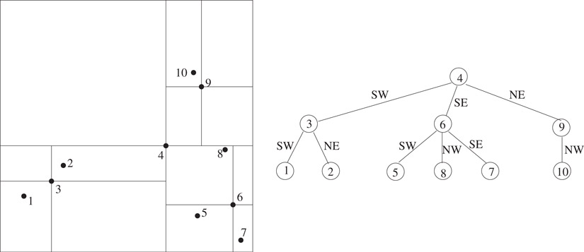
Figure 20.1A two dimensional set of points and a corresponding point quadtree.
If all the input points are known in advance, it is easy to choose the points for subdivision so as to construct a height balanced tree. A simple way to do this is to sort the points with one of the coordinates, say x, as the primary key and the other coordinate, say y, as the secondary key. The first subdivision point is chosen to be the median of this sorted data. This will ensure that none of the children of the root node receives more than half the points. In O(n) time, such a sorted list can be created for each of the four resulting subregions. As the total work at every level of the tree is bounded by O(n), and there are at most O(log n) levels in the tree, a height balanced point quadtree can be built in O(n log n) time. Generalization to d dimensions is immediate, with O(dn log n) run time.
The recursive structure of a point quadtree immediately suggests an algorithm for searching. To search for a point, compare it with the point stored at the root. If they are different, the comparison immediately suggests the subregion containing the point. The search is directed to the corresponding child of the root node. Thus, search follows a path in the quadtree until either the point is discovered, or a leaf node is reached. The run time is bounded by O(dh), where h is the height of the tree.
To insert a new point not already in the tree, first conduct a search for it which ends in a leaf node. The leaf node now corresponds to a region containing two points. One of them is chosen for subdividing the region and the other is inserted as a child of the node corresponding to the subregion it falls in. The run time for point insertion is also bounded by O(dh), where h is the height of the tree after insertion. One can also construct the tree itself by repeated insertions using this procedure. Similar to binary search trees, the run time under a random sequence of insertions is expected to be O(n log n) [6]. Overmars and van Leeuwen [7] present algorithms for constructing and maintaining optimized point quadtrees irrespective of the order of insertions.
Deletion in point quadtrees is much more complex. The point to be deleted is easily identified by a search for it. The difficulty lies in identifying a point in its subtree to take the place of the deleted point. This may require nontrivial readjustments in the subtree underneath. The reader interested in deletion in point quadtrees is referred to [8]. An analysis of the expected cost of various types of searches in point quadtrees is presented by Flajolet et al. [9].
For the remainder of the chapter, we will focus on quadtree data structures that use equal subdivision of the underlying space, called region quadtrees. This is because we regard Bentley’s multidimensional binary search trees [2], also called k-d trees, to be superior to point quadtrees. The k-d tree is a binary tree where a region is subdivided into two based only on one of the dimensions. If the dimension used for subdivision is cyclically rotated at consecutive levels in the tree, and the subdivision is chosen to be consistent with the point quadtree, then the resulting tree would be equivalent to the point quadtree but without the drawback of large degree (2d in d dimensions). Thus, it can be argued that point quadtrees are contained in k-d trees. Furthermore, recent results on compressed region quadtrees indicate that it is possible to simultaneously achieve the advantages of both region and point quadtrees. In fact, region quadtrees are the most widely used form of quadtrees despite their dependence on the spatial distribution of the underlying data. While their use posed theoretical inconvenience—it is possible to create as large a worst-case tree as desired with as little as three points—they are widely acknowledged as the data structure of choice for practical applications. We will outline some of these recent developments and outline how good practical performance and theoretical performance guarantees can both be achieved using region quadtrees.
The region quadtree for n points in d dimensions is defined as follows: Consider a hypercube large enough to enclose all the points. This region is represented by the root of the d-dimensional quadtree. The region is subdivided into 2d subregions of equal size by bisecting along each dimension. Each of these regions containing at least one point is represented as a child of the root node. The same procedure is recursively applied to each child of the root node. The process is terminated when a region contains only a single point. This data structure is also known as the point region quadtree, or PR-quadtree for short [10]. At times, we will simply use the term quadtree when the tree implied is clear from the context. The region quadtree corresponding to a two dimensional set of points is shown in Figure 20.2. Once the enclosing cube is specified, the region quadtree is unique. The manner in which a region is subdivided is independent of the specific location of the points within the region. This makes the size of the quadtree sensitive to the spatial distribution of the points.
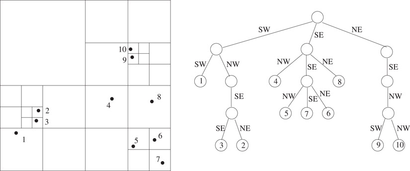
Figure 20.2A two dimensional set of points and the corresponding region quadtree.
Before proceeding further, it is useful to establish a terminology to describe the type of regions that correspond to nodes in the quadtree. Call a hypercubic region containing all the points the root cell. Define a hierarchy of cells by the following: The root cell is in the hierarchy. If a cell is in the hierarchy, then the 2d equal-sized cubic subregions obtained by bisecting along each dimension of the cell are also called cells and belong to the hierarchy (see Figure 20.3 for an illustration of the cell hierarchy in two dimensions). We use the term subcell to describe a cell that is completely contained in another. A cell containing the subcell is called a supercell. The subcells obtained by bisecting a cell along each dimension are called the immediate subcells with respect to the bisected cell. Also, a cell is the immediate supercell of any of its immediate subcells. We can treat a cell as a set of all points in space contained in the cell. Thus, we use C ⊆ D to indicate that the cell C is a subcell of the cell D and C ⊂ D to indicate that C is a subcell of D but C ≠ D. Define the length of a cell C, denoted length(C), to be the span of C along any dimension. An important property of the cell hierarchy is that, given two arbitrary cells, either one is completely contained in the other or they are disjoint. cells are considered disjoint if they are adjacent to each other and share a boundary.
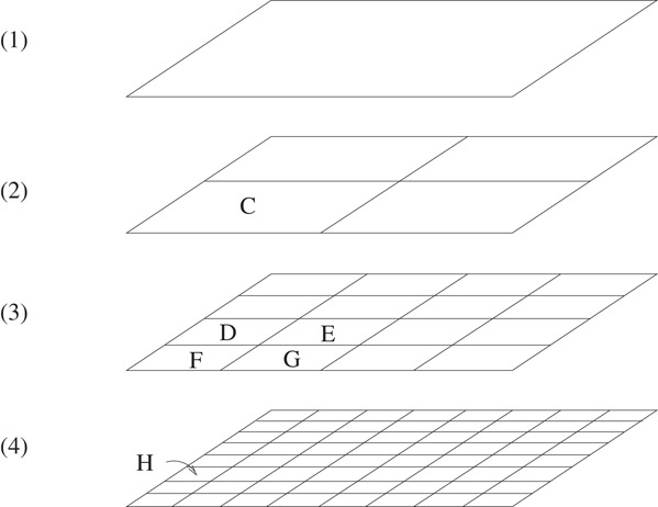
Figure 20.3Illustration of hierarchy of cells in two dimensions. Cells D, E, F and G are immediate subcells of C. Cell H is an immediate subcell of D, and is a subcell of C.
Each node in a quadtree corresponds to a subcell of the root cell. Leaf nodes correspond to largest cells that contain a single point. There are as many leaf nodes as the number of points, n. The size of the quadtree cannot be bounded as a function of n, as it depends on the spatial distribution. For example, consider a data set of 3 points consisting of two points very close to each other and a faraway point located such that the first subdivision of the root cell will separate the faraway point from the other two. Then, depending on the specific location and proximity of the other two points, a number of subdivisions may be necessary to separate them. In principle, the location and proximity of the two points can be adjusted to create as large a worst-case tree as desired. In practice, this is an unlikely scenario due to limits imposed by computer precision.
From this example, it is intuitively clear that a large number of recursive subdivisions may be required to separate points that are very close to each other. In the worst case, the recursive subdivision continues until the cell sizes are so small that a single cell cannot contain both the points irrespective of their location. Subdivision is never required beyond this point, but the points may be separated sooner depending on their actual location. Let s be the smallest distance between any pair of points and D be the length of the root cell. An upper bound on the height of the quadtree is obtained by considering the worst-case path needed to separate a pair of points which have the smallest pairwise distance. The length of the smallest cell that can contain two points s apart in d dimensions is (see Figure 20.4 for a two and three dimensional illustration). The paths separating the closest points may contain recursive subdivisions until a cell of length smaller than is reached. Since each subdivision halves the length of the cells, the maximum path length is given by the smallest k for which , or . For a fixed number of dimensions, the worst-case path length is . Since the tree has n leaves, the number of nodes in the tree is bounded by . In the worst case, D is proportional to the largest distance between any pair of points. Thus, the height of a quadtree is bounded by the logarithm of the ratio of the largest pairwise distance to the smallest pairwise distance. This ratio is a measure of the degree of nonuniformity of the distribution.
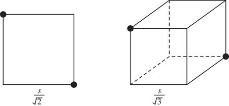
Figure 20.4Smallest cells that could possibly contain two points that are a distance s apart in two and three dimensions.
Search, insert and delete operations in region quadtrees are rather straightforward. To search for a point, traverse a path from root to a leaf such that each cell on the path encloses the point. If the leaf contains the point, it is in the quadtree. Otherwise, it is not. To insert a point not already in the tree, search for the point which terminates in a leaf. The leaf node corresponds to a region which originally had one point. To insert a new point which also falls within the region, the region is subdivided as many times as necessary until the two points are separated. This may create a chain of zero or more length below the leaf node followed by a branching to separate the two points. To delete a point present in the tree, conduct a search for the point which terminates in a leaf. Delete the leaf node. If deleting the node leaves its parent with a single child, traverse the path from the leaf to the root until a node with at least two children is encountered. Delete the path below the level of the child of this node. Each of the search, insert and delete operations takes O(h) time, where h is the height of the tree. Construction of a quadtree can be done either through repeated insertions, or by constructing the tree level by level starting from the root. In either case, the worst case run time is . We will not explore these algorithms further in favor of superior algorithms to be described later.
20.2.3Compressed Quadtrees and Octrees
In an n-leaf tree where each internal node has at least two children, the number of nodes is bounded by 2n − 1. The size of quadtrees is distribution dependent because there can be internal nodes with only one child. In terms of the cell hierarchy, a cell may contain all its points in a small volume so that, recursively subdividing it may result in just one of the immediate subcells containing the points for an arbitrarily large number of steps. Note that the cells represented by nodes along such a path have different sizes but they all enclose the same points. In many applications, all these nodes essentially contain the same information as the information depends only on the points the cell contains. This prompted the development of compressed quadtrees, which are obtained by compressing each such path into a single node. Therefore, each node in a compressed quadtree is either a leaf or has at least two children. The compressed quadtree corresponding to the quadtree of Figure 20.2 is depicted in Figure 20.5. Compressed quadtrees originated from the work of Clarkson [11] in the context of the all nearest neighbors problem and further studied by Aluru and Sevilgen [12].
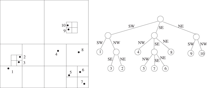
Figure 20.5The two-dimensional set of points from Figure 20.2, and the corresponding compressed quadtree.
A node v in the compressed quadtree is associated with two cells, large cell of v (L(v)) and small cell of v (S(v)). They are the largest and smallest cells that enclose the points in the subtree of the node, respectively. When S(v) is subdivided, it results in at least two non-empty immediate subcells. For each such subcell C resulting from the subdivision, there is a child u such that L(u) = C. Therefore, L(u) at a node u is an immediate subcell of S(v) at its parent v. A node is a leaf if it contains a single point and the small cell of a leaf node is the hypothetical cell with zero length containing the point.
The size of a compressed quadtree is bounded by O(n). The height of a compressed quadtree has a lower bound of Ω(log n) and an upper bound of O(n). Search, insert and delete operations on compressed quadtrees take O(h) time. In practice, the height of a compressed quadtree is significantly smaller than suggested by the upper bound because (a) computer precision limits restrict the ratio of largest pairwise distance to smallest pairwise distance that can be represented, and (b) the ratio of length scales represented by a compressed quadtree of height h is at least 2h:1. In most practical applications, the height of the tree is so small that practitioners use representation schemes that allow only trees of constant height [13,14] or even assume that the height is constant in algorithm analysis [15]. For instance, a compressed octree of height 20 allows potentially leaf nodes and a length scale of .
Though compressed quadtrees are described as resulting from collapsing chains in quadtrees, such a procedure is not intended for compressed quadtree construction. Instead, algorithms for direct construction of compressed quadtrees in O(dn log n) time will be presented, which can be used to construct quadtrees efficiently if necessary. To obtain a quadtree from its compressed version, identify each node whose small cell is not identical to its large cell and replace it by a chain of nodes corresponding to the hierarchy of cells that lead from the large cell to the small cell.
20.2.4Cell Orderings and Space-Filling Curves
We explore a suitable one dimensional ordering of cells and use it in conjunction with spatial ordering to develop efficient algorithms for compressed quadtrees. First, define an ordering for the immediate subcells of a cell. In two dimensions, we use the order SW, NW, SE and NE. The same ordering has been used to order the children of a node in a two dimensional quadtree (Figures 20.2 and 20.5). Now consider ordering two arbitrary cells. If one of the cells is contained in the other, the subcell precedes the supercell. If the two cells are disjoint, the smallest supercell enclosing both the cells contains them in different immediate subcells of it. Order the cells according to the order of the immediate subcells containing them. This defines a total order on any collection of cells with a common root cell. It follows that the order of leaf regions in a quadtree corresponds to the left-or-right order in which the regions appear in our drawing scheme. Similarly, the ordering of all regions in a quadtree corresponds to the postorder traversal of the quadtree. These concepts naturally extend to higher dimensions. Note that any ordering of the immediate subcells of a cell can be used as foundation for cell orderings.
Ordering of cells at a particular resolution in the manner described above can be related to space filling curves. Space filling curves are proximity preserving mappings from a multidimensional uniform cell decomposition to a one dimensional ordering. The path implied in the multidimensional space by the linear ordering, that is, the sequence in which the multidimensional cells are visited according to the linear ordering, forms a non-intersecting curve. Of particular interest is Morton ordering, also known as the Z-space filling curve [16]. The Z-curves for 2 × 2, 4 × 4 and 8 × 8 cell decompositions are shown in Figure 20.6. Consider a square two dimensional region and its 2k×2k cell decomposition. The curve is considered to originate in the lower left corner and terminate in the upper right corner. The curve for a 2k × 2k grid is composed of four grid curves one in each quadrant of the 2k × 2k grid and the tail of one curve is connected to the head of the next as shown in the figure. The order in which the curves are connected is the same as the order of traversal of the 2 × 2 curve. Note that Morton ordering of cells is consistent with the cell ordering specified above. Other space filling curves orderings such as graycode [17] and Hilbert [18] curve can be used and quadtree ordering schemes consistent with these can also be utilized. We will continue to utilize the Z-curve ordering as it permits a simpler bit interleaving scheme which will be presented and exploited later.
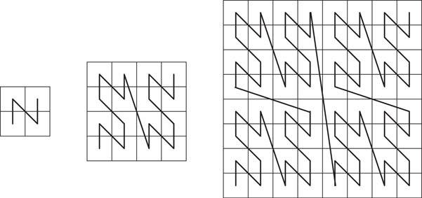
Figure 20.6Z-curve for 2 × 2, 4 × 4 and 8 × 8 cell decompositions.
Algorithms on compressed quadtree rely on the following operation due to Clarkson [11]:
Lemma 20.1
Let R be the product of d intervals I1 × I2 × ··· × Id, that is, R is a hyperrectangular region in d dimensional space. The smallest cell containing R can be found in O(d) time, which is constant for any fixed d.
The procedure for computing the smallest cell uses floor, logarithm and bitwise exclusive-or operations. An extended RAM model is assumed in which these are considered constant time operations. The reader interested in proof of Lemma 20.1 is referred to [11,19]. The operation is useful in several ways. For example, the order in which two points appear in the quadtree as per our ordering scheme is independent of the location of other points. To determine the order for two points, say (x1, x2, …, xd) and (y1, y2, …, yd), find the smallest cell that contains [x1, y1] × [x2, y2] × ··· × [xd, yd]. The points can then be ordered according to its immediate subcells that contain the respective points. Similarly, the smallest cell containing a pair of other cells, or a point and a cell, can be determined in O(d) time.
20.2.5Construction of Compressed Quadtrees
20.2.5.1A Divide-and-Conquer Construction Algorithm
Let T1 and T2 be two compressed quadtrees representing two distinct sets S1 and S2 of points. Let r1 (respectively, r2) be the root node of T1 (respectively, T2). Suppose that L(r1) = L(r2), that is, both T1 and T2 are constructed starting from a cell large enough to contain S1∪S2. A compressed quadtree T for S1∪S2 can be constructed in O(|S1| + |S2|) time by merging T1 and T2.
To merge T1 and T2, start at their roots and merge the two trees recursively. Suppose that at some stage during the execution of the algorithm, node u in T1 and node v in T2 are being considered. An invariant of the merging algorithm is that L(u) and L(v) cannot be disjoint. Furthermore, it can be asserted that S(u) ∪ S(v) ⊆ L(u) ∩ L(v). In merging two nodes, only the small cell information is relevant because the rest of the large cell (L(v) − S(v)) is empty. For convenience, assume that a node may be empty. If a node has less than 2d children, we may assume empty nodes in place of the absent children. Four distinct cases arise:
•Case I: If a node is empty, the result of merging is simply the tree rooted at the other node.
•Case II: If S(u) = S(v), the corresponding children of u and v have the same large cells which are the the immediate subcells of S(u) (or equivalently, S(v)). In this case, merge the corresponding children one by one.
•Case III: If S(v) ⊂ S(u), the points in v are also in the large cell of one of the children of u. Thus, this child of u is merged with v. Similarly, if S(u) ⊂ S(v), u is merged with the child of v whose large cell contains S(u).
•Case IV: If S(u) ∩ S(v) = Ø, then the smallest cell containing both S(u) and S(v) contains S(u) and S(v) in different immediate subcells. In this case, create a new node in the merged tree with its small cell as the smallest cell that contains S(u) and S(v) and make u and v the two children of this node. Subtrees of u and v are disjoint and need not be merged.
Lemma 20.2
Two compressed quadtrees with a common root cell can be merged in time proportional to the sum of their sizes.
Proof. The merging algorithm presented above performs a preorder traversal of each compressed quadtree. The whole tree may not need to be traversed because in merging a node, it may be determined that the whole subtree under the node directly becomes a subtree of the resulting tree. In every step of the merging algorithm, we advance on one of the trees after performing at most O(d) work. Thus, the run time is proportional to the sum of the sizes of the trees to be merged.■
To construct a compressed quadtree for n points, scan the points and find the smallest and largest coordinate along each dimension. Find a region that contains all the points and use this as the root cell of every compressed quadtree constructed in the process. Recursively construct compressed quadtrees for points and the remaining points and merge them in O(dn) time. The compressed quadtree for a single point is a single node v with the root cell as L(v). The run time satisfies the recurrence
resulting in O(dn log n) run time.
20.2.5.2Bottom-up Construction
To perform a bottom-up construction, first compute the order of the points in O(dn log n) time using any optimal sorting algorithm and the ordering scheme described previously. The compressed quadtree is then incrementally constructed starting from the single node tree for the first point and inserting the remaining points as per the sorted list. During the insertion process, keep track of the most recently inserted leaf. Let p be the next point to be inserted. Starting from the most recently inserted leaf, traverse the path from the leaf to the root until the first node v such that p ∈ L(v) is encountered. Two possibilities arise:
•Case I: If p ∉ S(v), then p is in the region L(v) − S(v), which was empty previously. The smallest cell containing p and S(v) is a subcell of L(v) and contains p and S(v) in different immediate subcells. Create a new node u between v and its parent and insert p as a child of u.
•Case II: If p ∈ S(v), v is not a leaf node. The compressed quadtree presently does not contain a node that corresponds to the immediate subcell of S(v) that contains p, that is, this immediate subcell does not contain any of the points previously inserted. Therefore, it is enough to insert p as a child of v corresponding to this subcell.
Once the points are sorted, the rest of the algorithm is identical to a post-order walk on the final compressed quadtree with O(d) work per node. The number of nodes visited per insertion is not bounded by a constant but the number of nodes visited over all insertions is O(n), giving O(dn) run time. Combined with the initial sorting of the points, the tree can be constructed in O(dn log n) time.
Fast algorithms for operations on quadtrees can be designed by simultaneously keeping track of spatial ordering and one dimensional ordering of cells in the compressed quadtree. The spatial ordering is given by the compressed quadtree itself. In addition, a balanced binary search tree (BBST) is maintained on the large cells of the nodes to enable fast cell searches. Both the trees consist of the same nodes and this can be achieved by allowing each node to have pointers corresponding to compressed quadtree structure and pointers corresponding to BBST structure.
20.2.6.1Point and Cell Queries
Point and cell queries are similar since a point can be considered to be a zero length cell. A node v is considered to represent cell C if S(v) ⊆ C ⊆ L(v). The node in the compressed quadtree representing the given cell is located using the BBST. Traverse the path in the BBST from the root to the node that is being searched in the following manner: To decide which child to visit next on the path, compare the query cell with the large and small cells at the node. If the query cell precedes the small cell in cell ordering, continue the search with the left child. If it succeeds the large cell in cell ordering, continue with the right child. If it lies between the small cell and large cell in cell ordering, the node represents the query cell. As the height of a BBST is O(log n), the time taken for a point or cell query is O(d log n).
20.2.6.2Insertions and Deletions
As points can be treated as cells of zero length, insertion and deletion algorithms will be discussed in the context of cells. These operations are meaningful only if a cell is inserted as a leaf node or deleted if it is a leaf node. Note that a cell cannot be deleted unless all its subcells are previously deleted from the compressed quadtree.
20.2.6.3Cell Insertion
To insert a given cell C, first check whether it is represented in the compressed quadtree. If not, it should be inserted as a leaf node. Create a node v with S(v) = C and first insert v in the BBST using a standard binary search tree insertion algorithm. To insert v in the compressed quadtree, first find the BBST successor of v, say u. Find the smallest cell D containing C and the S(u). Search for cell D in the BBST and identify the corresponding node w. If w is not a leaf, insert v as a child of w in compressed quadtree. If w is a leaf, create a new node w′ such that S(w′) = D. Nodes w and v become the children of w′ in the compressed quadtree. The new node w′ should be inserted in the BBST. The overall algorithm requires a constant number of insertions and searches in the BBST, and takes O(d log n) time.
20.2.6.4Cell Deletion
As in insertion, the cell should be deleted from the BBST and the compressed quadtree. To delete the cell from BBST, the standard deletion algorithm is used. During the execution of this algorithm, the node representing the cell is found. The node is deleted from the BBST only if it is present as a leaf node in the compressed quadtree. If the removal of this node from the compressed quadtree leaves its parent with only one child, the parent is deleted as well. Since each internal node has at least two children, the delete operation cannot propagate to higher levels in the compressed quadtree.
20.2.7Practical Considerations
In most practical applications, the height of a region quadtree is rather small because the spatial resolution provided by a quadtree is exponential in its height. This can be used to design schemes that will greatly simplify and speedup quadtree algorithms.
Consider numbering the 22k cells of a 2k × 2k two dimensional cell decomposition in the order specified by the Z-curve using integers 0…4k − 1 (Figure 20.6). Represent each cell in the cell space using a coordinate system with k bits for each coordinate. From the definition of the Z-curve, it follows that the number of a cell can be obtained by interleaving the bits representing the x and y coordinates of the cell, starting from the x coordinate. For example, (3, 5) = (011, 101) translates to 011011 = 27. The procedure can be extended to higher dimensions. If (x1, x2, …xd) represents the location of a d dimensional cell, the corresponding number can be obtained by taking bit representations of x1, x2, …xd, and interleaving them.
The same procedure can be described using uncompressed region quadtrees. Label the 2d edges connecting a node to its children with bit strings of length d. This is equivalent to describing the immediate subcells of a cell using one bit for each coordinate followed by bit interleaving. A cell can then be described using concatenation of the bits along the path from the root to the cell. This mechanism can be used to simultaneously describe cells at various length scales. The bit strings are conveniently stored in groups of 32 or 64 bits using integer data types. This creates a problem in distinguishing certain cells. For instance, consider distinguishing cell “000” from cell “000000” in an octree. To ensure each bit string translates to a unique integer when interpreted as a binary number, it is prefixed by a 1. It also helps in easy determination of the length of a bit string by locating the position of the leftmost 1. This leads to a representation that requires dk + 1 bits for a d dimensional quadtree with a height of at most k. Such a representation is very beneficial because primitive operations on cells can be implemented using bit operations such as and, or, exclusive-or etc. For example, 128 bits (4 integers on a 32 bit computer and 2 integers on a 64 bit computer) are sufficient to describe an octree of height 42, which allows representation of length scales .
The bit string based cell representation greatly simplifies primitive cell operations. In the following, the name of a cell is also used to refer to its bit representation:
•Check if C1 ⊆ C2. If C2 is a prefix of C1, then C1 is contained in C2, otherwise not.
•Find the smallest cell enclosing C1 and C2. This is obtained by finding the longest common prefix of C1 and C2 whose length is 1modd.
•Find the immediate subcell of C1 that contains C2. If dl + 1 is the number of bits representing C1, the required immediate subcell is given by the first (d + 1)l + 1 bits of C2.
Consider n points in a root cell and let k denote the largest resolution to be used. Cells are not subdivided further even if they contain multiple points. From the coordinates of a point, it is easy to compute the leaf cell containing it. Because of the encoding scheme used, if cell C should precede cell D in the cell ordering, the number corresponding to the binary interpretation of the bit string representation of C is smaller than the corresponding number for D. Thus, cells can be sorted by simply treating them as numbers and ordering them accordingly.
Finally, binary search trees and the attendant operations on them can be completely avoided by using hashing to directly access a cell. An n leaf compressed quadtree has at most 2n − 1 nodes. Hence, an array of that size can be conveniently used for hashing. If all cells at the highest resolution are contained in the quadtree, that is, n = dk, then an array of size 2n − 1 can be used to directly index cells. Further details of such representation are left as an exercise to the reader.
20.3Spatial Queries with Region Quadtrees
In this section, we consider a number of spatial queries involving point data, and algorithms for them using compressed region quadtrees.
Range queries are commonly used in database applications. Database records with d keys can be represented as points in d-dimensional space. In a range query, ranges of values are specified for all or a subset of keys with the objective of retrieving all the records that satisfy the range criteria. Under the mapping of records to points in multidimensional space, the ranges define a (possibly open-ended) hyperrectangular region. The objective is to retrieve all the points that lie in this query region.
As region quadtrees organize points using a hierarchy of cells, the range query can be answered by finding a collection of cells that are both fully contained in the query region and completely encompass the points in it. This can be achieved by a top-down traversal of the compressed region quadtree starting from the root. To begin with, is empty. Consider a node v and its small cell S(v). If S(v) is outside the query region, the subtree underneath it can be safely discarded. If S(v) is completely inside the query region, it is added to . All points in the subtree of S(v) are within the query region and reported as part of the output. If S(v) overlaps with the query region but is not contained in it, each child of v is examined in turn.
If the query region is small compared to the size of the root cell, it is likely that a path from the root is traversed where each cell on the path completely contains the query region. To avoid this problem, first compute the smallest cell encompassing the query region. This cell can be searched in O(d log n) time using the cell search algorithm described before, or perhaps in O(d) time if the hashing/indexing technique is applicable. The top-down traversal can start from the identified cell. When the cell is subdivided, at least two of its children represent cells that overlap with the query region. Consider a child cell and the part of the query region that is contained in it. The same idea can be recursively applied by finding the smallest cell that encloses this part of the query region and directly finding this cell rather than walking down a path in the tree to reach there. This ensures that the number of cells examined during the algorithm is . To see why, consider the cells examined as organized into a tree based on subcell-supercell relationships. The leaves of the tree are the collection of cells . Each cell in the tree is the smallest cell that encloses a subregion of the query region. Therefore, each internal node has at least two children. Consequently, the size of the tree, or the number of cells examined in answering the range query is . For further study of range queries and related topics, see [17,20, 21].
Next, we turn our attention to a number of spatial queries which we categorize as group queries. In group queries, a query to retrieve points that bear a certain relation to a query point is specified. The objective of the group query is to simultaneously answer n queries with each input point treated as a query point. For example, given n points, finding the nearest neighbor of each point is a group query. While the run time of performing the query on an individual point may be large, group queries can be answered more efficiently by intelligently combining the work required in answering queries for the individual points. Instead of presenting a different algorithm for each query, we show that the same generic framework can be used to solve a number of such queries. The central idea behind the group query algorithm is to realize run time savings by processing queries together for nearby points. Consider a cell C in the compressed quadtree and the (as yet uncomputed) set of points that result from answering the query for each point in C. The algorithm keeps track of a collection of cells of size as close to C as possible that is guaranteed to contain these points. The algorithm proceeds in a hierarchical manner by computing this information for cells of decreasing sizes (see Figure 20.7).
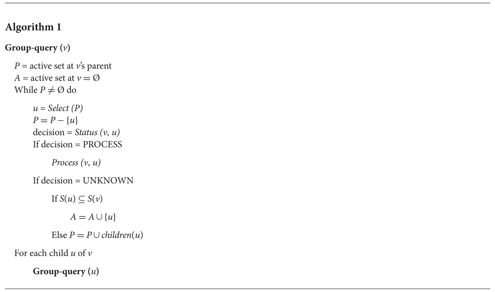
Figure 20.7Unified algorithm for the group queries.
A node u is said to be resolved with respect to node v if, either all points in S(u) are in the result of the query for all points in S(v) or none of the points in S(u) is in the result of the query for any point in S(v). Define the active set of a node v to be the set of nodes u that cannot be resolved with respect to v such that S(u) ⊆ S(v) ⊆ L(u). The algorithm uses a depth first search traversal of the compressed quadtree. The active set of the root node contains itself. The active set of a node v is calculated by traversing portions of the subtrees rooted at the nodes in the active set of its parent. The functions Select, Status and Process used in the algorithm are designed based on the specific group query. When considering the status of a node u with respect to the node v, the function Status(v,u) returns one of the following three values:
•PROCESS – If S(u) is in the result of the query for all points in S(v)
•DISCARD – If S(u) is not in the result of the query for all points in S(v)
•UNKNOWN – If neither of the above is true
If the result is either PROCESS or DISCARD, the children of u are not explored. Otherwise, the size of S(u) is compared with the size of S(v). If S(u) ⊆ S(v), then u is added to the set of active nodes at v for consideration by v’s children. If S(u) is larger, then u’s children are considered with respect to v. It follows that the active set of a leaf node is empty, as the length of its small cell is zero. Therefore, entire subtrees rooted under the active set of the parent of a leaf node are explored and the operation is completed for the point inhabiting that leaf node. The function Process(v,u) reports all points in S(u) as part of the result of query for each point in S(v).
The order in which nodes are considered is important for proving the run time of some operations. The function Select is used to accommodate this.
20.3.2Spherical Region Queries
Given a query point and a distance r > 0, the spherical region query is to find all points that lie within a distance of r from the query point. The group version of the spherical region query is to take n points and a distance r > 0 as input, and answer spherical region queries with respect to each of the input points.
A cell D may contain points in the spherical region corresponding to some points in cell C only if the smallest distance between D and C is less than r. If the largest distance between D and C is less than r, then all points in D are in the spherical region of every point in C. Thus, the function Status(v,u) is defined as follows: If the largest distance between S(u) and S(v) is less than r, return PROCESS. If the smallest distance between S(u) and S(v) is greater than r, return DISCARD. Otherwise, return UNKNOWN. Processing u means including all the points in u in the query result for each point in v. For this query, no special selection strategy is needed.
For computing the k-nearest neighbors of each point, some modifications to the algorithm presented in Figure 20.7 are necessary. For each node w in P, the algorithm keeps track of the largest distance between S(v) and S(w). Let dk be the kth smallest of these distances. If the number of nodes in P is less than k, then dk is set to ∞. The function Status(v,u) returns DISCARD if the smallest distance between S(v) and S(u) is greater than dk. The option PROCESS is never used. Instead, for a leaf node, all the points in the nodes in its active set are examined to select the k nearest neighbors. The function Select picks the largest cell in P, breaking ties arbitrarily.
Computing k-nearest neighbors is a well-studied problem [11,22]. The algorithm presented here is equivalent to Vaidya’s algorithm [22,23], even though the algorithms appear to be very different on the surface. Though Vaidya does not consider compressed quadtrees, the computations performed by his algorithm can be related to traversal on compressed quadtrees and a proof of the run time of the presented algorithm can be established by a correspondence with Vaidya’s algorithm. The algorithm runs in O(kn) time. The proof is quite elaborate, and omitted for lack of space. For details, see [22,23]. The special case of n = 1 is called the all nearest neighbor query, which can be computed in O(n) time.
20.4Image Processing Applications
Quadtrees are ubiquitously used in image processing applications. Consider a two dimensional square array of pixels representing a binary image with black foreground and white background (Figure 20.8). As with region quadtrees used to represent point data, a hierarchical cell decomposition is used to represent the image. The pixels are the smallest cells used in the decomposition and the entire image is the root cell. The root cell is decomposed into its four immediate subcells and represented by the four children of the root node. If a subcell is completely composed of black pixels or white pixels, it becomes a leaf in the quadtree. Otherwise, it is recursively decomposed. If the resolution of the image is 2k × 2k, the height of the resulting region quadtree is at most k. A two dimensional image and its corresponding region quadtree are shown in Figure 20.8. In drawing the quadtree, the same ordering of the immediate subcells of a cell into SW, NW, SE and NE quadrants is followed. Each node in the tree is colored black, white, or gray, depending on if the cell consists of all black pixels, all white pixels, or a mixture of both black and white pixels, respectively. Thus, internal nodes are colored gray and leaf nodes are colored either black or white.
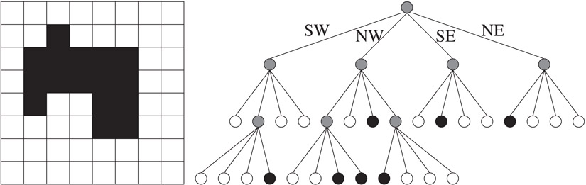
Figure 20.8A two dimensional array of pixels, and the corresponding region quadtree.
Each internal node in the image quadtree has four children. For an image with n leaf nodes, the number of internal nodes is . For large images, the space required for storing the internal nodes and the associated pointers may be expensive and several space-efficient storage schemes have been investigated. These include storing the quadtree as a collection of leaf cells using the Morton numbering of cells [24], or as a collection of black leaf cells only [25,26], and storing the quadtree as its preorder traversal [27]. Iyengar et al. introduced a number of space-efficient representations of image quadtrees including forests of quadtrees [28,29], translation invariant data structures [30–32] and virtual quadtrees [33].
The use of quadtrees can be easily extended to grayscale images and color images. Significant space savings can be realized by choosing an appropriate scheme. For example, 2r gray levels can be encoded using r bits. The image can be represented using r binary valued quadtrees. Because adjacent pixels are likely to have gray levels that are closer, a gray encoding of the 2r levels is advantageous over a binary encoding [27]. The gray encoding has the property that adjacent levels differ by one bit in the gray code representation. This should lead to larger blocks having the same value for a given bit position, leading to shallow trees.
20.4.1Construction of Image Quadtrees
Region quadtrees for image data can be constructed using an algorithm similar to the bottom-up construction algorithm for point region quadtrees described in Section 20.2.5. In fact, constructing quadtrees for image data is easier because the smallest cells in the hierarchical decomposition are given by the pixels and all the pixels can be read by the algorithm as the image size is proportional to the number of pixels. Thus, quadtree for region data can be built in time linear in the size of the image, which is optimal. The pixels of the image are scanned in Morton order which eliminates the need for the sorting step in the bottom-up construction algorithm. It is wasteful to build the complete quadtree with all pixels as leaf nodes and then compact the tree by replacing maximal subtrees having all black or all white pixels with single leaf nodes, though such a method would still run in linear time and space. By reading the pixels in Morton order, a maximal black or white cell can be readily identified and the tree can be constructed using only such maximal cells as leaf nodes [8]. This will limit the space used by the algorithm to the final size of the quadtree.
20.4.2Union and Intersection of Images
The union of two images is the overlay of one image over another. In terms of the array of pixels, a pixel in the union is black if the pixel is black in at least one of the images. In the region quadtree representation of images, the quadtree corresponding to the union of two images should be computed from the quadtrees of the constituent images. Let I1 and I2 denote the two images and T1 and T2 denote the corresponding region quadtrees. Let T denote the region quadtree of the union of I1 and I2. It is computed by a preorder traversal of T1 and T2 and examining the corresponding nodes/cells. Let v1 in T1 and v2 in T2 be nodes corresponding to the same region. There are three possible cases:
•Case I: If v1 or v2 is black, the corresponding node is created in T and is colored black. If only one of them is black and the other is gray, the gray node will contain a subtree underneath. This subtree need not be traversed.
•Case II: If v1 (respectively, v2) is white, v2 (respectively, v1) and the subtree underneath it (if any) is copied to T.
•Case III: If both v1 and v2 are gray, then the corresponding children of v1 and v2 are considered.
The tree resulting from the above merging algorithm may consist of unnecessary subdivisions of a cell consisting of completely black pixels. For example, if a region is marked gray in both T1 and T2 but each of the four quadrants of the region is black in at least one of T1 and T2, then the node corresponding to the region in T will have four children colored black. This is unnecessary as the node itself can be colored black and should be considered a leaf node. Such adjustments need not be local and may percolate up the tree. For instance, consider a checker board image of 2k × 2k pixels with half black and half white pixels such that the north, south, east and west neighbors of a black pixel are white pixels and vice versa. Consider another checker board image with black and white interchanged. The quadtree for each of these images is a full 4-ary tree of level k. But overlaying one image over another produces one black square of size 2k × 2k. The corresponding quadtree should be a single black node. However, merging initially creates a full 4-ary tree of depth k. To compact the tree resulting from merging to create the correct region quadtree, a bottom-up traversal is performed. If all children of a node are black, then the children are removed and the node is colored black.
The intersection of two images can be computed similarly. A pixel in the intersection of two images is black only if the corresponding pixels in both the images are black. For instance, the intersection of the two complementary checkerboard images described above is a single white cell of size 2k × 2k. The algorithm for intersection can be obtained by interchanging the roles of black and white in the union algorithm. Similarly, a bottom-up traversal is used to detect nodes all of whose children are white, remove the children, and color the node white. Union and intersection algorithms can be easily generalized to multiple images.
Quadtree representation of images facilitates certain types of rotation and scaling operations. Rotations on images are often performed in multiples of 90 degrees. Such a rotation has the effect of changing the quadrants of a region. For example, a 90 degree clockwise rotation changes the SW, NW, SE, NE quadrants to NW, NE, SW, SE quadrants, respectively. This change should be recursively carried out for each region. Hence, a rotation that is a multiple of 90 degrees can be effected by simply reordering the child pointers of each node. Similarly, scaling by a power of two is trivial using quadtrees since it is simply a loss of resolution. For other linear transformations, see the work of Hunter [34,35].
20.4.4Connected Component Labeling
Two black pixels of a binary image are considered adjacent if they share a horizontal or vertical boundary. A pair of black pixels is said to be connected if there is a sequence of adjacent pixels leading from one to the other. A connected component is a maximal set of black pixels where every pair of pixels is connected. The connected component labeling problem is to find the connected components of a given image and give each connected component a unique label. Identifying the connected components of an image is useful in object counting and image understanding. Samet developed algorithms for connected component labeling using quadtrees [36].
Let B and W denote the number of black nodes and white nodes, respectively, in the quadtree. Samet’s connected component labeling algorithm works in three stages:
1.Establish the adjacency relationships between pairs of black pixels.
2.Identify a unique label for each connected component. This can be thought of as computing the transitive closure of the adjacency relationships.
3.Label each black cell with the corresponding connected component.
The first stage is carried out using a postorder traversal of the quadtree during which adjacent black pixels are discovered and identified by giving them the same label. To begin with, all the black nodes are unlabeled. When a black region is considered, black pixels adjacent to it in two of the four directions, say north and east, are searched. The post order traversal of the tree traverses the regions in Morton order. Thus when a region is encountered, its south and west adjacent black regions (if any) would have already been processed. At that time, the region would have been identified as a neighbor. Thus, it is not necessary to detect adjacency relationships between a region and its south or west adjacent neighbors.
Suppose the postorder traversal is currently at a black node or black region R. Adjacent black regions in a particular direction, say north, are identified as follows. First, identify the adjacent region of the same size as R that lies to the north of R. Traverse the quadtree upwards to the root to identify the first node on the path that contains both the regions, or equivalently, find the lowest common ancestor of both the regions in the quadtree. If such a node does not exist, R has no north neighbor and it is at the boundary of the image. Otherwise, a child of this lowest common ancestor will be a region adjacent to the north boundary of R and of the same size as or larger than R. If this region is black, it is part of the same connected component as R. If neither the region nor R is currently labeled, create a new label and use it for both. If only one of them is labeled, use the same label for the other. If they are both already labeled with the same label, do nothing. If they are both already labeled with different labels, the label pair is recorded as corresponding to an adjacency relationship. If the region is gray, it is recursively subdivided and adjacent neighbors examined to find all black regions that are adjacent to R. For each black neighbor, the labeling procedure described above is carried out.
The run time of this stage of the algorithm depends on the time required to find the north and east neighbors. This process can be improved using the smallest-cell primitive described earlier. However, Samet proved that the average of the maximum number of nodes visited by the above algorithm for a given black region and a given direction is smaller than or equal to 5, under the assumption that a black region is equally likely to occur at any position and level in the quadtree [36]. Thus, the algorithm should take time proportional to the size of the quadtree, that is, O(W + B) time.
Stage two of the algorithm is best performed using the union-find data structure [37]. Consider all the labels that are used in stage one and treat them as singleton sets. For every pair of labels recorded in stage one, perform a find operation to find the two sets that contain the labels currently, and do a union operation on the sets. At the end of stage two, all labels used for the same connected component will be grouped together in one set. This can be used to provide a unique label for each set (called the set label), and subsequently identify the set label for each label. The number of labels used is bounded by B. The amortized run time per operation using the union-find data structure is given by the inverse Ackermann’s function [37], a constant (≤ 4) for all practical purposes. Therefore, the run time of stage two can be considered to be O(B). Stage three of the algorithm can be carried out by another postorder traversal of the quadtree to replace the label of each black node with the corresponding set label in O(B + W) time. Thus, the entire algorithm runs in O(B + W) time.
20.5Scientific Computing Applications
Region quadtrees are widely used in scientific computing applications. Most of the problems are three dimensional, prompting the development of octree based methods. In fact, some of the practical techniques and shortcuts presented earlier for storing region quadtrees and bit string representation of cells owe their origin to applications in scientific computing.
Octree are used in many ways in scientific computing applications. In many scientific computing applications, the behavior of a physical system is captured through either (1) a discretization of the space using a finite grid, followed by determining the quantities of interest at each of the grid cells, or (2) computing the interactions between a system of (real or virtual) particles which can be related to the behavior of the system. The former are known as grid-based methods and typically correspond to the solution of differential equations. The latter are known as particle-based methods and often correspond to the solution of integral equations. Both methods are typically iterative and the spatial information, such as the hierarchy of grid cells or the spatial distribution of the particles, often changes from iteration to iteration.
Examples of grid-based methods include finite element methods, finite difference methods, multigrid methods and adaptive mesh refinement methods. Many applications use a cell decomposition of space as the grid or grid hierarchy and the relevance of octrees for such applications is immediate. Algorithms for construction of octrees and methods for cell insertions and deletions are all directly applicable to such problems. It is also quite common to use other decompositions, especially for the finite-element method. For example, a decomposition of a surface into triangular elements is often used. In such cases, each basic element can be associated with a point (for example, the centroid of a triangle), and an octree can be built using the set of points. Information on the neighboring elements required by the application is then related to neighborhood information on the set of points.
Particle based methods include such simulation techniques as molecular dynamics, smoothed particle hydrodynamics, and N-body simulations. These methods require many of the spatial queries discussed in this chapter. For example, van der Waal forces between atoms in molecular dynamics fall off so rapidly with increasing distance (inversely proportional to the sixth power of the distance between atoms) that a cutoff radius is employed. In computing the forces acting on an individual atom, van der Waal forces are taken into account only for atoms that lie within the cutoff radius. The list of such atoms is typically referred to as the neighbor list. Computing neighbor lists for all atoms is just a group spherical region query, already discussed before. Similarly, k-nearest neighbors are useful in applications such as smoothed particle hydrodynamics. In this section, we further explore the use of octrees in scientific computing by presenting an optimal algorithm for the N-body problem.
The N-body problem is defined as follows: Given n bodies and their positions, where each pair of bodies interact with a force inversely proportional to the square of the distance between them, compute the force on each body due to all other bodies. A direct algorithm for computing all pairwise interactions requires O(n2) time. Greengard’s fast multipole method [15], which uses an octree data structure, reduces this complexity by approximating the interaction between clusters of bodies instead of computing individual interactions. For each cell in the octree, the algorithm computes a multipole expansion and a local expansion. The multipole expansion at a cell C, denoted ϕ(C), is the effect of the bodies within C on distant bodies. The local expansion at C, denoted ψ(C), is the effect of all distant bodies on bodies within C.
The N-body problem can be solved in O(n) time using a compressed octree [12]. For two cells C and D which are not necessarily of the same size, define a predicate well-separated(C, D) to be true if D’s multipole expansion converges at any point in C, and false otherwise. If two cells are not well-separated, they are proximate. Similarly, two nodes v1 and v2 in the compressed octree are said to be well-separated if and only if S(v1) and S(v2) are well-separated. Otherwise, we say that v1 and v2 are proximate.
For each node v in the compressed octree, the multipole expansion ϕ(v) and the local expansion ψ(v) need to be computed. Both ϕ(v) and ψ(v) are with respect to the cell S(v). The multipole expansions can be computed by a simple bottom-up traversal in O(n) time. For a leaf node, its multipole expansion is computed directly. At an internal node v, ϕ(v) is computed by aggregating the multipole expansions of the children of v.
The algorithm to compute the local expansions is given in Figure 20.9. The astute reader will notice that this is the same group query algorithm described in Section 20.3, reproduced here again with slightly different notation for convenience. The computations are done using a top-down traversal of the tree. To compute local expansion at node v, consider the set of nodes that are proximate to its parent, which is the proximity set, P(parent(v)). The proximity set of the root node contains only itself. Recursively decompose these nodes until each node is either (1) well-separated from v or (2) proximate to v and the length of the small cell of the node is no greater than the length of S(v). The nodes satisfying the first condition form the interaction set of v, I(v) and the nodes satisfying the second condition are in the proximity set of v, P(v). In the algorithm, the set E(v) contains the nodes that are yet to be processed. Local expansions are computed by combining parent’s local expansion and the multipole expansions of the nodes in I(v). For the leaf nodes, potential calculation is completed by using the direct method.
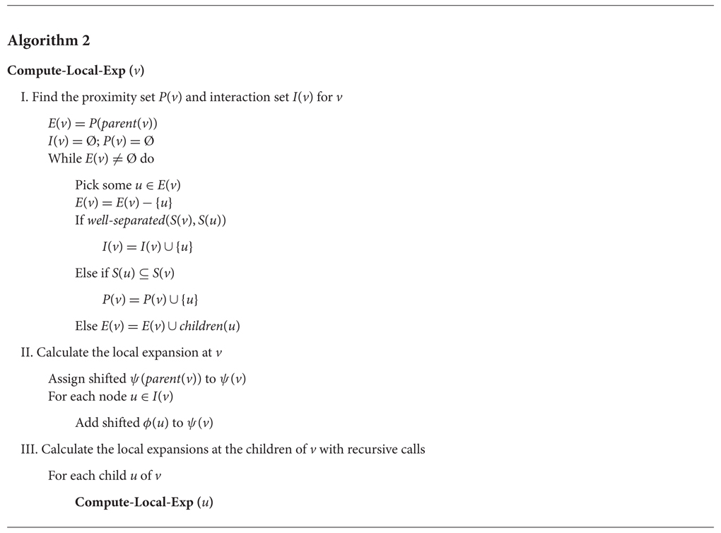
Figure 20.9Algorithm for calculating local expansions of all nodes in the tree rooted at v.
The following terminology is used in analyzing the run time of the algorithm. The set of cells that are proximate to C and having same length as C is called the proximity set of C and is defined by P= (C) = {D | length(C) = length(D), ¬well - separated(C, D)}. The superscript “ = ” is used to indicate that cells of the same length are being considered. For node v, define the proximity set P(v) as the set of all nodes proximate to v and having the small cell no greater than and large cell no smaller than S(v). More precisely, P(v) = {w | ¬well-separated(S(v), S(w)), length(S(w)) ≤ length(S(v)) ≤ length(L(w))}. The interaction set I(v) of v is defined as I(v) = {w | well-separated(S(v), S(w)), [w ∈ P(parent(v))∨{∃u ∈ P(parent(v)), w is a descendant of u, ¬well - sep(v, parent(w)), length(S(v)) < length(S(parent(w)))}]}. We use parent(w) to denote the parent of the node w.
The algorithm achieves O(n) run time for any predicate well - separated that satisfies the following three conditions:
1.The relation well-separated is symmetric for equal length cells, that is, length(C) = length(D)⇒ well-separated(C, D) = well-separated(D, C).
2.For any cell C, |P=(C)| is bounded by a constant.
3.If two cells C and D are not well-separated, any two cells C′ and D′ such that C ⊆ C′ and D ⊆ D′ are not well-separated as well.
These three conditions are respected by the various well-separatedness criteria used in N-body algorithms and in particular, Greengard’s algorithm. In N-body methods, the well-separatedness decision is solely based on the geometry of the cells and their relative distance and is oblivious to the number of bodies or their distribution within the cells. Given two cells C and D of the same length, if D can be approximated with respect to C, then C can be approximated with respect to D as well, as stipulated by Condition C1. The size of the proximity sets of cells of the same length should be O(1) as prescribed by Condition C2 in order that an O(n) algorithm is possible. Otherwise, an input that requires processing the proximity sets of Ω(n) such cells can be constructed, making an O(n) algorithm impossible. Condition C3 merely states that two cells C′ and D′ are not well-separated unless every subcell of C′ is well-separated from every subcell of D′.
Lemma 20.3
For any node v in the compressed octree, |P(v)| = O(1).
Proof. Consider any node v. Each u ∈ P(v) can be associated with a unique cell C ∈ P=(S(v)) such that S(u) ⊆ C. This is because any subcell of C which is not a subcell of S(u) is not represented in the compressed octree. It follows that |P(v)| ≤ |P= (S(v))| = O(1) (by Condition C2).■
Lemma 20.4
The sum of interaction set sizes over all nodes in the compressed octree is linear in the number of nodes in the compressed octree, that is, .
Proof. Let v be a node in the compressed octree. Consider any w ∈ I(v), either w ∈ P(parent(v)) or w is in the subtree rooted by a node u ∈ P(parent(v)). Thus,
Consider these two summations separately. The bound for the first summation is easy; From Lemma 20.3, |P(parent(v))| = O(1). So,
The second summation should be explored more carefully.
In what follows, we bound the size of the set M(w) = {v | w ∈ I(v), w∉P(parent(v))} for any node.
Since w ∉ P(parent(v)), there exists a node u ∈ P(parent(v)) such that w is in the subtree rooted by u. Consider parent(w): The node parent(w) is either u or a node in the subtree rooted at u. In either case, length(S(parent(w))) ≤ length(S(parent(v))). Thus, for each v ∈ M(w), there exists a cell C such that S(v) ⊆ C ⊆ S(parent(v)) and length(S(parent(w))) = length(C). Further, since v and parent(w) are not well-separated, C and S(parent(w)) are not well-separated as well by Condition C3. That is to say S(parent(w)) ∈ P=(C) and C ∈ P=(S(parent(w))) by Condition C1. By Condition C2, we know that |P=(S(parent(w)))| = O(1). Moreover, for each cell C ∈ P=(S(parent(w))), there are at most 2d choices of v because length(C) ≤ length(S(parent(v))). As a result, |M(w)| ≤ 2d × O(1) = O(1) for any node w. Thus, .■
Theorem 20.1
Given a compressed octree for n bodies, the N-body problem can be solved in O(n) time.
Proof. Computing the multipole expansion at a node takes constant time and the number of nodes in the compressed octree is O(n). Thus, total time required for the multipole expansion calculation is O(n). The nodes explored during the local expansion calculation at a node v are either in P(v) or I(v). In both cases, it takes constant time to process a node. By Lemmas 20.3 and 20.4, the total size of both sets for all nodes in the compressed octree is bounded by O(n). Thus, local expansion calculation takes O(n) time. As a conclusion, the running time of the fast multipole algorithm on the compressed octree takes O(n) time irrespective of the distribution of the bodies.■
It is interesting to note that the same generic algorithmic framework is used for spherical region queries, all nearest neighbors, k-nearest neighbors and solving the N-body problem. While the proofs are different, the algorithm also provides optimal solution for k-nearest neighbors and the N-body problem.
While this chapter is focused on applications of quadtrees and octrees in image processing and scientific computing applications, they are used for many other types of spatial data and in the context of numerous other application domains. A detailed study of the design and analysis of quadtree based data structures and their applications can be found in [4,5].
This work was supported, in part, by the National Science Foundation under grant ACI-0306512.
1.A. Klinger. Optimizing methods in statistics, chapter Patterns and search statistics, pages 303–337. 1971.
2.J. L. Bentley. Multidimensional binary search trees used for associative searching. Communications of the ACM, 18(9):509–517, 1975.
3.G. M. Hunter. Efficient computation and data structures for graphics. PhD thesis, Princeton University, Princeton, NJ, USA, 1978.
4.H. Samet. The Design and Analysis of Spatial Data Structures. Addison-Wesley, Reading, MA, 1989.
5.H. Samet. Applications of Spatial Data Structures: Computer Graphics, Image Processing, and GIS. Addison-Wesley, Reading, MA, 1989.
6.R. A. Finkel and J. L. Bentley. Quad trees: a data structure for retrieval on composite key. Acta Informatica, 4(1):1–9, 1974.
7.M. H. Overmars and J. van Leeuwen. Dynamic multi-dimentional data structures based on quad- and K-D trees. Acta Informatica, 17:267–285, 1982.
8.H. Samet. Deletion in two-dimentional quad trees. Communications of the ACM, 23(12):703–710, 1980.
9.P. Flajolet, G. Gonnet, C. Puech, and J. M. Robson. The analysis of multidimensional searching in quad-trees. In Alok Aggarwal, editor, Proceedings of the 2nd Annual ACM-SIAM Symposium on Discrete Algorithms (SODA ’90), pages 100–109, San Francisco, CA, USA, 1990.
10.H. Samet, A. Rosenfeld, C. A. Shaffer, and R. E. Webber. Processing geographic data with quadtrees. In Seventh Int. Conference on Pattern Recognition, pages 212–215. IEEE Computer Society Press, 1984.
11.K. L. Clarkson. Fast algorithms for the all nearest neighbors problem. In 24th Annual Symposium on Foundations of Computer Science (FOCS ’83), pages 226–232, 1982.
12.S. Aluru and F. Sevilgen. Dynamic compressed hyperoctrees with application to the N-body problem. In Springer-Verlag Lecture Notes in Computer Science, volume 19, 1999.
13.B. Hariharan, S. Aluru, and B. Shanker. A scalable parallel fast multipole method for analysis of scattering from perfect electrically conducting surfaces. In SC’2002 Conference CD, http://www.supercomp.org, 2002.
14.M. Warren and J. Salmon. A parallel hashed-octree N-body algorithm. In Proceedings of Supercomputing ’93, 1993.
15.L. F. Greengard. The Rapid Evaluation of Potential Fields in Particle Systems. MIT Press, 1988.
16.G. M. Morton. A computer oriented geodetic data base and a new technique in file sequencing. Technical report, IBM, Ottawa, Canada, 1966.
17.C. Faloutsos. Gray codes for partial match and range queries. IEEE Transactions on Software Engineering, 14(10):1381–1393, 1988.
18.D. Hilbert. Uber die stegie abbildung einer linie auf flachenstuck. 38:459–460, 1891.
19.S. Aluru, J. L. Gustafson, G. M. Prabhu, and F. E. Sevilgen. Distribution-independent hierarchical algorithms for the N-body problem. The Journal of Supercomputing, 12(4):303–323, 1998.
20.J. A. Orenstein and T. H. Merrett. A class of data structures for associative searching. In Proceedings of the Fourth ACM SIGACT-SIGMOD Symposium on Principles of Database Systems, pages 181–190, 1984.
21.B. Pagel, H. Six, H. Toben, and P. Widmayer. Toward an analysis of range query performance in spatial data structures. In Proceedings of the Twelfth ACM SIGACT-SIGMOD-SIGART Symposium on Principles of Database Systems, pages 214–221, 1993.
22.P. M. Vaidya. An optimal algorithm for the All-Nearest-Neighbors problem. In 27th Annual Symposium on Foundations of Computer Science, pages 117–122. IEEE, 1986.
23.P. M. Vaidya. An O(n log n) algorithm for the All-Nearest-Neighbors problem. Discrete and Computational Geometry, 4:101–115, 1989.
24.A. Klinger and M. L. Rhodes. Organization and access of image data by areas. IEEE Transactions on Pattern Analysis and Machine Intelligence, 1(1):50–60, 1979.
25.I. Gargantini. An effective way to represent quadtrees. Communications of the ACM, 25(12):905–910, 1982.
26.I. Gargantini. Translation, rotation and superposition of linear quadtrees. International Journal of Man-Machine Studies, 18(3):253–263, 1983.
27.E. Kawaguchi, T. Endo, and J. Matsunaga. Depth-first expression viewed from digital picture processing. IEEE Transactions on Pattern Analysis and Machine Intelligence, 5(4):373–384, 1983.
28.N. K. Gautier, S. S. Iyengar, N. B. Lakhani, and M. Manohar. Space and time efficiency of the forest-of-quadtrees representation. Image and Vision Computing, 3:63–70, 1985.
29.V. Raman and S. S. Iyengar. Properties and applications of forests of quadtrees for pictorial data representation. BIT, 23(4):472–486, 1983.
30.S. S. Iyengar and H. Gadagkar. Translation invariant data structure for 3-D binary images. Pattern Recognition Letters, 7:313–318, 1988.
31.D. S. Scott and S. S. Iyengar. A new data structure for efficient storing of images. Pattern Recognition Letters, 3:211–214, 1985.
32.D. S. Scott and S. S. Iyengar. Tid – a translation invariant data structure for storing images. Communications of the ACM, 29(5):418–429, 1986.
33.L. P. Jones and S. S. Iyengar. Space and time efficient virtual quadtrees. IEEE Transactions on Pattern Analysis and Machine Intelligence, 6:244–247, 1984.
34.G. M. Hunter and K. Steiglitz. Linear transformation of pictures represented by quad trees. Computer Graphics and Image Processing, 10(3):289–296, 1979.
35.G. M. Hunter and K. Steiglitz. Operations on images using quad trees. IEEE Transactions on Pattern Analysis and Machine Intelligence, 1(2):143–153, 1979.
36.H. Samet. Connected component labeling using quadtrees. Journal of the ACM, 28(3):487–501, 1981.
37.R. E. Tarjan. Efficiency of a good but not linear disjoint set union algorithm. Journal of the ACM, 22:215–225, 1975.
*This chapter has been reprinted from first edition of this Handbook, without any content updates.