
Shigang Chen
University of Florida
Description of Bloom Filter•Performance Metrics•False-Positive Ratio and Optimal k
Description of CBF•Counter Size and Counter Overflow
Bloom-1 Filter•Impact of Word Size•Bloom-1 Versus Bloom with Small k•Bloom-1 versus Bloom with Optimal k•Bloom-g: A Generalization of Bloom-1•Bloom-g versus Bloom with Small k•Bloom-g versus Bloom with Optimal k•Discussion•Using Bloom-g in a Dynamic Environment
10.5Other Bloom Filter Variants
Improving Space Efficiency•Reducing False-Positive Ratio•Improving Read/Write Efficiency•Reducing Hash Complexity•Bloom Filter for Dynamic Set
The Bloom filter is a compact data structure for fast membership check against a data set. It was first proposed by Burton Howard Bloom in 1970 [1]. As illustrated in Figure 10.1, given an element, it answers such query: is the element in the set? The output is either “no” or “maybe.” In other words, it may give false positives, but false negatives are not possible.
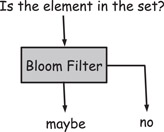
Figure 10.1Black box view of a Bloom filter.
The Bloom filter has wide applications in routing-table lookup [2–4], online traffic measurement [5,6], peer-to-peer systems [7,8], cooperative caching [9], firewall design [10], intrusion detection [11], bioinformatics [12], database query processing [13,14], stream computing [15], distributed storage system [16], and so on [17,18]. For example, a firewall may be configured with a large watch list of addresses that are collected by an intrusion detection system. If the requirement is to log all packets from those addresses, the firewall must check each arrival packet to see if the source address is a member of the list. Another example is routing-table lookup. The lengths of the prefixes in a routing table range from 8 to 32. A router can extract 25 prefixes of different lengths from the destination address of an incoming packet, and it needs to determine which prefixes are in the routing tables [2]. Some traffic measurement functions require the router to collect the flow labels [6,19], such as source/destination address pairs or address/port tuples that identify TCP flows. Each flow label should be collected only once. When a new packet arrives, the router must check whether the flow label extracted from the packet belongs to the set that has already been collected before. As a last example for the membership check problem, we consider the context-based access control (CBAC) function in Cisco routers [20]. When a router receives a packet, it may want to first determine whether the addresses/ports in the packet have a matching entry in the CBAC table before performing the CBAC lookup.
In all of the previous examples, we face the same fundamental problem. For a large data set, which may be an address list, an address prefix table, a flow label set, a CBAC table, or other types of data, we want to check whether a given element belongs to this set or not. If there is no performance requirement, this problem can be easily solved using conventional exact-checking data structures such as binary search [21] (which stores the set in a sorted array and uses binary search for membership check) or a traditional hash table [22] (which uses linked lists to resolve hash collision). However, these approaches are inadequate if there are stringent speed and memory requirements.
Modern high-end routers and firewalls implement their per-packet operations mostly in hardware. They are able to forward each packet in a couple of clock cycles. To keep up with such high throughput, many network functions that involve per-packet processing also have to be implemented in hardware. However, they cannot store the data structures for membership check in DRAM because the bandwidth and delay of DRAM access cannot match the packet throughput at the line speed. Consequently, the recent research trend is to implement membership check in the high-speed on-die cache memory, which is typically SRAM. The SRAM is however small and must be shared among many online functions. This prevents us from storing a large data set directly in the form of a sorted array or a hash table. On the other hand, a Bloom filter can provide compact membership checking with reasonable precision. For example, it has 1% false-positive probability with fewer than 10 bits per element and 0.1% false-positive probability with fewer than 15 bits per element.
10.2.1Description of Bloom Filter
A Bloom filter is a space-efficient data structure to encode a set. It includes an array B of m bits, which are initialized to zeros. The array stores the membership information of a set as follows: each member e of the set is mapped to k bits that are randomly selected from B through k hash functions, Hi(e), 1 ≤ i ≤ k, whose range is [0, m − 1).*. To encode the membership information of e, the bits, B[H1(e)], …, B[Hk(e)], are set to ones. These are called the “membership bits” in B for the element e. Figure 10.2 illustrates how a set {a, b, c} is encoded to a Bloom filter with m = 16, k = 3.

Figure 10.2Encoding a set to a Bloom filter with k = 3.
To check the membership of an arbitrary element e′, if the k bits, B[Hi(e′)], 1 ≤ i ≤ k, are all ones, e′ is accepted to be a member of the set. Otherwise, it is denied. Continuing with the Bloom filter shown in Figure 10.2, we illustrate membership checking in the Bloom filter in Figure 10.3. As element a was previously encoded, the three bits B[H1(a)], B[H2(a)], B[H3(a)] were already set to ones. Therefore, a is accepted as a member. In the second example, as element d is not a member of the set {a, b, c}, chances are it will hit a zero in the array. Therefore, it is denied as a nonmember.

Figure 10.3Membership checking in a Bloom filter with encoded.
A Bloom filter doesn’t have false negative, meaning that a member element will always be accepted. The filter however may incur false positive, meaning that if it answers that an element is in the set, it may not be really in the set. As illustrated in the third example of Figure 10.3, element e is not a member of set {a, b, c}, but B[H1(e)], B[H2(e)], B[H3(e)] all happen to be ones, which were individually set by real members.
The performance of the Bloom filter is judged based on three criteria. The first one is the processing overhead, which is k memory accesses and k hash operations for each membership query. The overhead* limits the highest throughput that the filter can support. For example, as both SRAM and the hash function circuit may be shared among different network functions, it is important for them to minimize their processing overhead in order to achieve good system performance. The second performance criterion is the space requirement, which is the size m of the array B. Minimizing the space requirement to encode each member allows a network function to fit a large set in the limited SRAM space for membership check. The third criterion is the false-positive ratio or false-positive probability, which is the probability for a Bloom filter to erroneously accept a nonmember. There is a trade-off between the space requirement and the false-positive ratio. We can reduce the latter by allocating more memory.
We can treat the k hash functions logically as a single one that produces k⌈log2 m⌉ hash bits. For example, suppose m is 220, k = 3, and a hash routine outputs 64 bits. We can extract three 20-bit segments from the first 60 bits of a single hash output and use them to locate three bits in B. Hence, from now on, instead of specifying the number of hash functions required by a filter, we will state “the number of hash bits” that are needed, which is denoted as h. Table 10.1 summarizes the performance metrics of the Bloom filter. In the next subsection, we will show how the false-positive ratio in Table 10.1 is derived.
Table 10.1Performance Metrics of the Bloom Filter
|
Space |
Memory Access |
Hash Bits |
False-Positive Ratio |
|
m |
k |
k⌈ log2 m⌉ |
(1 − e−nk/m)k |
m, the size of the bit array; k, the number of membership bits (a.k.a. the number of hash functions); n, the number of elements encoded.
10.2.3False-Positive Ratio and Optimal k
We denote the false-positive ratio as fB. Assume that the hash functions generate fully random locations. The probability that a bit is not set to one by a hash function during the insertion of an element is 1 − (1/m), where m is the number of bits in the array. The probability that the bit remains zero after inserting n elements, each setting k bits to ones, is
Therefore, the probability that it is one is
For an arbitrary nonmember element, each of the k mapped positions has the above probability to be one. The probability of all of them being one, that is, the false-positive ratio, is often given as*
(10.1) |
|---|
Obviously, the false-positive ratio decreases as the size m of the array increases, and increases as the number n of elements encoded increases. The optimal value of k (denoted as k*) that minimizes the false-positive ratio can be derived by taking the first-order derivative on Equation 10.1 with respect to k, then letting the right side be zero, and solving the equation.
The result is
(10.2) |
|---|
Figure 10.4 shows the optimal k of the Bloom filter with respect to the load factor, which is defined as n/m. When the load factor is small, the optimal k can be very large. To avoid too many memory accesses, we may also set k as a small constant in practice. When the optimal k is used, the false-positive ratio becomes
(10.3) |
|---|
Figure 10.5 shows the false-positive ratio of the Bloom filter when the optimal k is used.

Figure 10.4Optimal number of hash functions (k) with respect to the load factor (n/m).

Figure 10.5False-positive ratio of the Bloom filter when optimal k is used.
If the requirement is to bound the false-positive ratio by a predefined value fREQ, that is, fB ≤ fREQ, we can determine the length of the Bloom filter by letting in Equation 10.3, which gives us
(10.4) |
|---|
Removing an element from the traditional Bloom filter is not possible. Each “1” bit in the Bloom filter may be shared by many elements, so we cannot simply reset the membership bits of the element to “0”, which may result in the removal of other elements. There are several ways to handle element deletion in the literature (see Section 10.5.5). In this section, we will discuss one of them in detail: the counting Bloom filter (CBF) [9].
A CBF encodes a set and enables element deletion, which is essentially an array C of l counters. All the counters are initially 0. Similar to the Bloom filter, each member e of the set is mapped to k counters that are randomly selected from C through k hash functions, Hi(e), 1 ≤ i ≤ k, whose range is [0, l − 1). To encode the membership information of e, the counters, C[H1(e)], …, C[Hk(e)], are incremented by one. To remove an element e from the set, the counters, C[H1(e)], …, C[Hk(e)], are decremented by one. To check the membership of an arbitrary element e′, if the k counters, C[Hi(e′)], 1 ≤ i ≤ k, are all nonzero, e′ is accepted to be a member of the set. Otherwise, it is denied.
Following the same analytical method in Section 10.2.3, we can see that the false-positive ratio of CBF is
(10.5) |
|---|
while the optimal k that minimize the false-positive ratio is
(10.6) |
|---|
where n is the number of elements encoded. A CBF with l counters has the same false-positive ratio as a traditional Bloom filter with m bits.
10.3.2Counter Size and Counter Overflow
As counters in CBF are preallocated, they have the same fixed size and hence counter overflow may happen. For example, suppose each counter consists of t bits. It can represent any count between 0 and 2t − 1. If a counter with value 2t − 1 is about to be incremented for encoding a new element, counter overflow will happen. A smaller value of t makes counter overflow more frequent. However, bigger t means more space: t times the space needed for a Bloom filter!
So our next question is, what is the best choice of t? Or, how small can each counter be to make counter overflow sufficiently rare? To answer this question, we first need to know how big a count value may become. Let c be a random variable which represents the value of an arbitrary counter after inserting n elements, each randomly increments k out of l counters. Obviously, c follows Binomial distribution, Bino(nk, 1/l).
The probability that the counter is greater or equal to y is
where indicates the descending factorial , i ≥ j. Clearly, . As a result, we can bound Prob{c ≥ y} by
(10.7) |
|---|
The probability that any counter is greater or equal to y is (assuming counter values are independent)
(10.8) |
|---|
where e is Euler’s number (e = 2.71828…). If the optimal k is used, that is, , we can further bound
(10.9) |
|---|
From Equation 10.9 and y = 2t, we can calculate the overflow probability of CBF with t-bit counters. The results are shown in Table 10.2. For example, when t = 4 and l = 220, the overflow probability is 1.43×10⁻⁹, which is extremely small. In other words, 4 bits per counter is enough for most practical values of l.
Table 10.2Probability for Any Counter to Overflow (Counter Value ≥ 2t) in a CBF with l Counters.
|
t = 2 |
t = 3 |
t = 4 |
t = 5 |
|
0.049 × l |
9.5×10⁻⁶ × l |
1.4×10⁻¹⁵ × l |
4.4×10−40 × l |
Each counter consists of t bits. The optimal k is used.
In practice, even if counter overflow ever happens, we can simply let it stay at the value. Although after many deletions this might lead to a situation where CBF allows a false negative (the count becomes 0 when it shouldn’t be), the probability of such a chain of events is usually extremely low.
CBF is a natural extension to the traditional Bloom filter and it is very easy to implement. One issue with CBF is its limited scalability. Because the counter array cannot be expanded, the maximal number of keys to be stored simultaneously in the filter must be known before constructing the filter. Once the designed capacity of the table is exceeded, the false-positive ratio will grow rapidly as more keys are inserted. As a result, even though CBF is designed for dynamic set, it works best when element population has a preknown maximum point.
Given the fact that Bloom filters have been applied so extensively, any improvement to their performance can potentially have a broad impact. In this section, we study a variant of the Bloom filter, called Bloom-1, which makes just one memory access to perform membership check [24–26]. Therefore, it can be configured to outperform the commonly used Bloom filter with constant k. We will show that when the required false-positive ratio is extremely small, the optimal k of the Bloom filter will be too large to be practical. Next, we generalize Bloom-1 to Bloom-g, which allows g memory accesses. We show that they can achieve the low false-positive ratio of the Bloom filter with optimal k, without incurring the same kind of high overhead. This family of Bloom filter variants is called the blocked Bloom filter. We discuss how blocked Bloom filters can be applied for static or dynamic data sets.
To check the membership of an element, a Bloom filter requires k memory accesses. We introduce the Bloom-1 filter, which requires one memory access for membership check. The basic idea is that, instead of mapping an element to k bits randomly selected from the entire bit array, we map it to k bits in a word that is randomly selected from the bit array. A word is defined as a continuous block of bits that can be fetched from the memory to the processor in one memory access. In today’s computer architectures, most general-purpose processors fetch words of 32 bits or 64 bits. Specifically designed hardware may access words of 72 bits or longer.
A Bloom-1 filter is an array B1 of l words, each of which is w bits long. The total number m of bits is l × w. To encode a member e during the filter setup, we first obtain a number of hash bits from e, and use log2 l hash bits to map e to a word in B1. It is called the “membership word” of e in the Bloom-1 filter. We then use k log2 w hash bits to further map e to k membership bits in the word and set them to ones. The total number of hash bits that are needed is log2 l + k log2 w. Suppose m = 220, k = 3, w = 26, and l = 214. Only 32 hash bits are needed, which is smaller than the 60 hash bits required in the previous Bloom filter example under similar parameters.
To check if an element e′ is a member in the set that is encoded in a Bloom-1 filter, we first perform hash operations on e′ to obtain log2 l + k log2 w hash bits. We use log2 l bits to locate its membership word in B1, and then use k log2 w bits to identify the membership bits in the word. If all membership bits are ones, it is considered to be a member. Otherwise, it is not.
The change from using k random bits in the array to using k random bits in a word may appear simple, but it is also fundamental. An important question is how it will affect the false-positive ratio and the processing overhead. A more interesting question is how it will open up new design space to configure various new filters with different performance properties. This is what we will investigate in depth.
The false-negative ratio of a Bloom-1 filter is also zero. The false-positive ratio fB1 of Bloom-1, which is the probability of mistakenly treating a nonmember as a member, is derived as follows: let F be the false-positive event that a nonmember e′ is mistaken for a member. The element e′ is hashed to a membership word. Let X be the random variable for the number of members that are mapped to the same membership word. Let x be a constant in the range of [0, n], where n is the number of members in the set. Assume we use fully random hash functions. When X = x, the conditional probability for F to occur is
(10.10) |
|---|
Obviously, X follows the binomial distribution, Bino(n, 1/l), because each of the n elements may be mapped to any of the l words with equal probabilities. Hence,
(10.11) |
|---|
Therefore, the false-positive ratio can be written as
(10.12) |
|---|
We first investigate the impact of word size w on the performance of a Bloom-1 filter. If n, l, and k are known, we can obtain the optimal word size that minimizes Equation 10.12. However, in reality, we can only decide the amount of memory (i.e., m) to be used for a filter, but cannot choose the word size once the hardware is installed. In the left plot of Figure 10.6, we compute the false-positive ratios of Bloom-1 under four word sizes: 32, 64, 72, and 256 bits, when the total amount of memory is fixed at m = 220 and k is set to 3. Note that the number of words, l = m/w, is inversely proportional to the word size.

Figure 10.6False-positive ratio with respect to word size w. Left plot: False-positive ratios for Bloom-1 under different word sizes. Right plot: Magnified false-positive ratios for Bloom-1 under different word sizes.
The horizontal axis in the figure is the load factor, n/m, which is the number of members stored by the filter divided by the number of bits in the filter. Since most applications require relatively small false-positive ratios, we zoom in at the load factor range of [0, 0.2] for a detailed look in the right plot of Figure 10.6. The computation results based on Equation 10.12 show that a larger word size helps to reduce the false-positive ratio. In that case, we should simply set w = m for the lowest false-positive ratio. However, in practice, w is given by the hardware, not a configurable parameter. Without losing generality, we choose w = 64 in our computations and simulations for the rest of this chapter.
10.4.3Bloom-1 Versus Bloom with Small k
Although the optimal k always yields the best false positive ratio of the Bloom filter, a small value of k is sometimes preferred to bound the processing overhead in terms of memory accesses and hash operations. We compare the performance of the Bloom-1 filter and the Bloom filter in both scenarios. In this section, we use the Bloom filter with k = 3 as the benchmark. Using k = 4, 5, … produces quantitatively different results, but the qualitative conclusion will stay the same.
We compare the performance of three types of filters: (1) B(k = 3), which represents a Bloom filter that uses three bits to encode each member; (2) B1(k = 3), which represents a Bloom-1 filter that uses three bits to encode each member; (3) B1(h = 3 log2 m), which represents a Bloom-1 filter that uses the same number of hash bits as B(k = 3) does.
Let k1* be the optimal value of k that minimizes the false-positive ratio of the Bloom-1 filter in Equation 10.12. For B1(h = 3 log2 m), we are allowed to use 3 log2 m hash bits, which can encode three or more membership bits in the filter. However, it is not necessary to use more than the optimal number k1* of membership bits. Hence, B1(h = 3 log2 m) actually uses the k that is closest to k1* to encode each member.
Table 10.3 presents numerical results of the number of memory accesses and the number of hash bits needed by the three filters for each membership query. They together represent the query overhead and control the query throughput. First, we compare B(k = 3) and B1(k = 3). The Bloom-1 filter saves not only memory accesses but also hash bits. For example, in these examples, B1(k = 3) requires about half of the hash bits needed by B(k = 3). When the hash routine is implemented in hardware, such as CRC [27], the memory access may become the performance bottleneck, particularly when the filter’s bit array is located off-chip or, even if it is on-chip, the bandwidth of the cache memory is shared by other system components. In this case, the query throughput of B1(k = 3) will be three times of the throughput of B(k = 3).
Table 10.3Query Overhead Comparison of Bloom-1 Filters and Bloom Filter with k = 3.
|
Number of Hash Bits |
||||
|
Data Structure |
Number of Memory Access |
m = 216 |
m = 220 |
m = 224 |
|
B(k = 3) |
3 |
48 |
60 |
72 |
|
B1(k = 3) |
1 |
28 |
32 |
36 |
|
B1(h = 3 log2 m) |
1 |
16–46 |
20–56 |
24–72 |
Next, we consider B1(h = 3 log2 m). Even though it still makes one memory access to fetch a word, the processor may check more than 3 bits in the word for a membership query. If the operations of hashing, accessing memory, and checking membership bits are pipelined and the memory access is the performance bottleneck, the throughput of B1(h = 3 log2 m) will also be three times of the throughput of B(k = 3).
Finally, we compare the false-positive ratios of the three filters in Figure 10.7. The figure shows that the overall performance of B1(k = 3) is comparable to that of B(k = 3), but its false-positive ratio is worse when the load factor is small. The reason is that concentrating the membership bits in one word reduces the randomness. B1(h = 3 log2 m) is better than B(k = 3) when the load factor is smaller than 0.1. This is because the Bloom-1 filter requires less number of hash bits on average to locate each membership bit than the Bloom filter does. Therefore, when available hash bits are the same, B1(h = 3 log2 m) is able to use a larger k than B(k = 3), as shown in Figure 10.8.

Figure 10.7Performance comparison in terms of false-positive ratio.
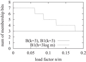
Figure 10.8Number of membership bits used by the filters.
10.4.4Bloom-1 versus Bloom with Optimal k
We can reduce the false-positive ratio of a Bloom filter or a Bloom-1 filter by choosing the optimal number of membership bits. From Equation 10.2, we find the optimal value k* that minimizes the false-positive ratio of a Bloom filter. From Equation 10.12, we can find the optimal value k1* that minimizes the false-positive ratio of a Bloom-1 filter. The values of k* and k1* with respect to the load factor are shown in Figure 10.9. When the load factor is less than 0.1, k1* is significantly smaller than k*.
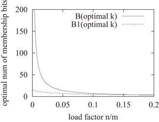
Figure 10.9Optimal number of membership bits with respect to the load factor.
We use B(optimal k) to denote a Bloom filter that uses the optimal number k* of membership bits and B1(optimal k) to denote a Bloom-1 filter that uses the optimal number k1* of membership bits.
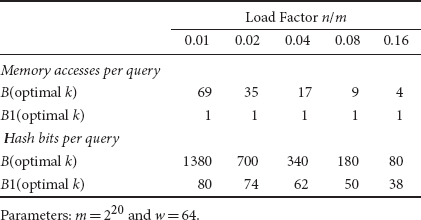
To make the comparison more concrete, we present the numerical results of memory access overhead and hashing overhead with respect to the load factor in Table 10.4. For example, when the load factor is 0.04, the Bloom filter requires 17 memory accesses and 340 hash bits to minimize its false-positive ratio, whereas the Bloom-1 filter requires only 1 memory access and 62 hash bits. In practice, the load factor is determined by the application requirement on the false-positive ratio. If an application requires a very small false-positive ratio, it has to choose a small load factor.
Table 10.4Query Overhead Comparison of Bloom-1 Filter and Bloom Filter with Optimal Number of Membership Bits
Next, we compare the false-positive ratios of B(optimal k) and B1(optimal k) with respect to the load factor in Figure 10.10. The Bloom filter has a much lower false-positive ratio than the Bloom-1 filter. On one hand, we must recognize the fact that, as shown in Table 10.4, the overhead for the Bloom filter to achieve its low false-positive ratio is simply too high to be practical. On the other hand, it raises a challenge for us to improve the design of the Bloom-1 filter so that it can match the performance of the Bloom filter at much lower overhead. In the next section, we generalize the Bloom-1 filter to allow performance-overhead trade-off, which provides flexibility for practitioners to achieve a lower false-positive ratio at the expense of modestly higher query overhead.

Figure 10.10False-positive ratios of the Bloom filter and the Bloom-1 filter with optimal k.
10.4.5Bloom-g: A Generalization of Bloom-1
As a generalization of Bloom-1 filter, a Bloom-g filter maps each member e to g words instead of one and spreads its k membership bits evenly in the g words. More specifically, we use g log2 l hash bits derived from e to locate g membership words, and then use k log2 w hash bits to locate k membership bits. The first one or multiple words are each assigned ⌈k/g⌉ membership bits, and the remaining words are each assigned ⌊k/g⌋ bits, so that the total number of membership bits is k.
To check the membership of an element e′, we have to access g words. Hence the query overhead includes g memory accesses and g log2 l + k log2 w hash bits.
The false-negative ratio of a Bloom-g filter is zero and the false-positive ratio fBg of the Bloom-g filter is derived as follows: each member encoded in the filter randomly selects g membership words. There are n members. Together they select gn membership words (with replacement). These words are called the “encoded words.” In each encoded word, k/g bits are randomly selected to be set as ones during the filter setup. To simplify the analysis, we use k/g instead of taking the ceiling or floor.
Now consider an arbitrary word D in the array. Let X be the number of times this word is selected as an encoded word during the filter setup. Assume we use fully random hash functions. When any member randomly selects a word to encode its membership, the word D has a probability of 1/l to be selected. Hence, X is a random number that follows the binomial distribution Bino(gn, 1/l). Let x be a constant in the range [0, gn].
(10.13) |
|---|
Consider an arbitrary nonmember e′. It is hashed to g membership words. A false positive happens when its membership bits in each of the g words are ones. Consider an arbitrary membership word of e′. Let F be the event that the k/g membership bits of e′ in this word are all ones. Suppose this word is selected for x times as an encoded word during the filter setup. We have the following conditional probability:
(10.14) |
|---|
The probability for F to happen is
(10.15) |
|---|
Element e′ has g membership words. Hence, the false-positive ratio is
(10.16) |
|---|
When g = k, exactly one bit is set in each membership word. This special Bloom-k is identical to a Bloom filter with k membership bits. (Note that Bloom-k may happen to pick the same membership word more than once. Hence, just like a Bloom filter, Bloom-k allows more than one membership bit in a word.) To prove this, we first let g = k, and Equation 10.16 becomes
(10.17) |
|---|
As m = lw, we have fBk = fB. In other words, a Bloom-k filter is identical to a Bloom filter.
10.4.6Bloom-g versus Bloom with Small k
We compare the performance and overhead of the Bloom-g filters and the Bloom filter with k = 3. Because the overhead of Bloom-g increases with g, it is highly desirable to use a small value for g. Hence, we focus on Bloom-2 and Bloom-3 filters as typical examples in the Bloom-g family.
We compare the following filters:
1.B(k = 3), the Bloom filter with k = 3;
2.B2(k = 3), the Bloom-2 filter with k = 3;
3.B2(h = 3 log2 m), the Bloom-2 filter that is allowed to use the same number of hash bits as B(k = 3) does.
In this section, we do not consider Bloom-3 because it is equivalent to B(k = 3), as we have discussed in Section 10.4.5.
From Equation 10.16, when g = 2, we can find the optimal value of k, denoted as k2*, that minimizes the false-positive ratio. Similar to B1(h = 3 log2 m), the filter B2(h = 3 log2 m) uses the k that is closest to k2* under the constraint that the number of required hash bits is less than or equal to 3 log2 m.
Table 10.5 compares the query overhead of three filters. The Bloom filter, B(k = 3), needs three memory accesses and 3 log2 m hash bits for each membership query. The Bloom-2 filter, B2(k = 3), requires two memory accesses and 2 log2 l + 3 log2 w hash bits. It is easy to see 2log2 l + 3log2 w = 3log2 m − log2 l < 3log2 m. Hence, B2(k = 3) incurs fewer memory accesses and fewer hash bits than B(k = 3). On the other hand, B2(h = 3 log2 m) uses the same number of hash bits as B(k = 3) does, but makes fewer memory accesses.
Table 10.5Query Overhead Comparison of Bloom-2 Filter and Bloom Filter with k = 3.
|
Number of Hash Bits |
||||
|
Data Structure |
Number of Memory Access |
m = 216 |
m = 220 |
m = 224 |
|
B(k = 3) |
3 |
48 |
60 |
72 |
|
B2(k = 3) |
2 |
38 |
46 |
54 |
|
B2(h = 3 log2 m) |
2 |
32–44 |
40–58 |
48–72 |
Figure 10.11 presents the false-positive ratios of B(k = 3), B2(k = 3), and B2(h = 3 log2 m). Figure 10.12 shows the number of membership bits used by the filters. The figures show that B(k = 3) and B2(k = 3) have comparable false-positive ratios in load factor range of [0.1,1], whereas B2(h = 3 log2 m) performs better in load factor range of [0.00005, 1]. For example, when the load factor is 0.04, the false-positive ratio of B(k = 3) is 1.5 × 10⁻³ and that of B2(k = 3) is 1.6 × 10⁻³, while the false-positive ratio of B2(h = 3 log2 m) is 3.1 × 10⁻⁴, about one-fifth of the other two. Considering that B2(h = 3 log2 m) uses the same number of hash bits as B(k = 3) but only two memory accesses per query, it is a very useful substitute of the Bloom filter to build fast and accurate data structures for membership check.

Figure 10.11False-positive ratios of Bloom filter and Bloom-2 filter.

Figure 10.12Number of membership bits used by the filters.
10.4.7Bloom-g versus Bloom with Optimal k
We now compare the Bloom-g filters and the Bloom filter when they use the optimal numbers of membership bits determined from Equations 10.1 and 10.16, respectively. We use B(optimal k) to denote a Bloom filter that uses the optimal number k* of membership bits to minimize the false-positive ratio. We use Bg(optimal k) to denote a Bloom-g filter that uses the optimal number kg* of membership bits, where g = 1, 2, or 3. Figure 10.13 compares their numbers of membership bits (i.e., k*, k1*, k2*, and k3*). It shows that the Bloom filter uses many more membership bits when the load factor is small.

Figure 10.13Optimal number of membership bits with respect to the load factor.
Next, we compare the filters in terms of query overhead. For 1 ≤ g ≤ 3, Bg(optimal k) makes g memory accesses and uses g log2 l + kg* log2 w hash bits per membership query. Numerical comparison is provided in Table 10.6. In order to achieve a small false-positive ratio, one has to keep the load factor small, which means that B(optimal k) will have to make a large number of memory accesses and use a large number of hash bits. For example, when the load factor is 0.08, it makes 9 memory accesses with 180 hash bits per query, whereas the Bloom-1, Bloom-2, and Bloom-3 filters make 1, 2, and 3 memory accesses with 50, 70, and 90 hash bits, respectively. When the load factor is 0.02, it makes 35 memory accesses with 700 hash bits, whereas the Bloom-1, Bloom-2, and Bloom-3 filters make just 1, 2, and 3 memory accesses with 74, 118 and 162 hash bits, respectively.
Table 10.6Query Overhead Comparison of Bloom Filter and Bloom-g Filter with Optimal k
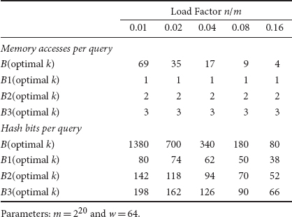
Figure 10.14 presents the false-positive ratios of the Bloom and Bloom-g filters. As we already showed in Section 10.4.4, B1(optimal k) performs worse than B(optimal k). However, the false-positive ratio of B2(optimal k) is very close to that of B(optimal k). Furthermore, the curve of B3(optimal k) is almost entirely overlapped with that of B(optimal k) for the whole load-factor range. The results indicate that with just two memory accesses per query, B2(optimal k) works almost as good as B(optimal k), even though the latter makes many more memory accesses.
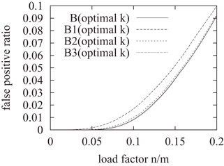
Figure 10.14False-positive ratios of Bloom and Bloom-g with optimal k.
The mathematical and numerical results demonstrate that Bloom-2 and Bloom-3 have smaller false-positive ratios than Bloom-1 at the expense of larger query overhead. Below we give an intuitive explanation: Bloom-1 uses a single hash to map each member to a word before encoding. It is well known that a single hash cannot achieve an evenly distributed load; some words will have to encode much more members than others, and some words may be empty as no members are mapped to them. This uneven distribution of members to the words is the reason for larger false positives. Bloom-2 maps each member to two words and splits the membership bits among the words. Bloom-3 maps each member to three words. They achieve better load balance such that most words will each encode about the same number of membership bits. This helps them improve their false-positive ratios.
10.4.9Using Bloom-g in a Dynamic Environment
In order to compute the optimal number of membership bits, we must know the values of n, m, w, and l. The values of m, w, and l are known once the amount of memory for the filter is allocated. The value of n is known only when the filter is used to encode a static set of members. In practice, however, the filter may be used for a dynamic set of members. For example, a router may use a Bloom filter to store a watch list of IP addresses, which are identified by the intrusion detection system as potential attackers. The router inspects the arrival packets and logs those packets whose source addresses belong to the list. If the watch list is updated once a week or at the midnight of each day, we can consider it as a static set of addresses during most of the time. However, if the system is allowed to add new addresses to the list continuously during the day, the watch list becomes a dynamic set. In this case, we do not have a fixed optimal value of k* for the Bloom filter. One approach is to set the number of membership bits to a small constant, such as three, which limits the query overhead. In addition, we should also set the maximum load factor to bound the false-positive ratio. If the actual load factor exceeds the maximum value, we allocate more memory and set up the filter again in a larger bit array.
The same thing is true for the Bloom-g filter. For a dynamic set of members, we do not have a fixed optimal number of membership bits, and the Bloom-g filter will also have to choose a fixed number of membership bits. The good news for the Bloom-g filter is that its number of membership bits is unrelated to its number of memory accesses. The flexible design allows it to use more membership bits while keeping the number of memory accesses small or even a constant one.
Comparing with the Bloom filter, we may configure a Bloom-g filter with more membership bits for a smaller false-positive ratio, while in the mean time keeping both the number of memory accesses and the number of hash bits smaller. Imagine a filter of 220 bits is used for a dynamic set of members. Suppose the maximum load factor is set to be 0.1 to ensure a small false-positive ratio. Figure 10.15 compares the Bloom filter with k = 3, the Bloom-1 filter with k = 6, and the Bloom-2 filter with k = 5. As new members are added over time, the load factor increases from 0 to 0.1. In this range of load factors, the Bloom-2 filter has significantly smaller false-positive ratios than the Bloom filter. When the load factor is 0.04, the false-positive ratio of Bloom-2 is just one-fourth of the false positive ratio of Bloom. Moreover, it makes fewer memory accesses per membership query. The Bloom-2 filter uses 58 hash bits per query, and the Bloom filter uses 60 bits. The false-positive ratios of the Bloom-1 filter are close to or slightly better than those of the Bloom filter. It achieves such performance by making just one memory access per query and uses 50 hash bits.

Figure 10.15False-positive ratios of the Bloom filter with k = 3, the Bloom-1 filter with k = 6, and the Bloom-2 filter with k = 5.
10.5Other Bloom Filter Variants
Since the Bloom filter was first proposed in 1970 [1], many variants have emerged to meet different requirements, such as supporting set updates, improving the space efficiency, memory access efficiency, false-positive ratio, and hash complexity of the Bloom filter. A comprehensive survey on Bloom filter variants and their applications can be found in Reference 18. Other Bloom filter variants were proposed to solve specific problems, for example, representing multisets [6,28–34] or sets with multiattribute members [35,36].
We will briefly introduce five categories of Bloom filter variants: the methods that aim to improve the space, hash, accuracy, and memory access efficiency of traditional Bloom filters, and the algorithms to support dynamic set.
10.5.1Improving Space Efficiency
Some Bloom filter variants aim to improve the space efficiency [37–39]. It has been proven that the Bloom filter is not space-optimal [17,39,40]. Pagh et al. [39] designed a new RAM data structure whose space usage is within a lower order term of the optimal value. Porat [38] designed a dictionary data structure that maps keys to values with optimal space. Mitzenmacher [37] proposed the compressed Bloom filters, which is suitable for message passing, for example, when the filters are transmitted through the Internet. The idea is to use a large, sparse Bloom filter at the sender/receiver, and compress/decompress the filter before/after transmission.
10.5.2Reducing False-Positive Ratio
Reducing the false-positive ratio of the Bloom filter is another subject of research. Lumetta and Mitzenmacher [41] proposed to use two choices (i.e., two sets of hash functions) for each element encoded in the Bloom filter. The idea is to pick the set of hash functions that produce the least number of ones, so as to reduce the false-positive ratio. This approach generates fewer false positives than the Bloom filter when the load factor is small, but it requires twice the number of hash bits and twice the number of memory access than the Bloom filter does.
Hao et al. [27] use partitioned hashing to divide members into several groups, each group with a different set of hash functions. Heuristic algorithms are used to find the “best” partition. However, this scheme requires the keys of member elements known as a prior to compute the final partition. Therefore, it only works well when members are inserted all at once and membership queries are performed afterwards.
Tabataba and Hashemi [42] proposed the Dual Bloom Filter to improve the false-positive ratio of a single Bloom filter. The idea is to use two equal sized Bloom filters to encode the set with different sets of hash functions. An element is considered a member only when both filters produce positives. In order to reduce the space usage for storing random numbers for different hash functions, the second Bloom filter encodes ones complemented values of the elements.
Lim et al. [43] use two cross-checking Bloom filters together with traditional Bloom filter to reduce the false positives. It first divides the set S to be encoded to two disjoint subsets A and B . Then they use three Bloom filters to encode S, A, B, respectively, denoted as F(S), F(A), F(B). Different hash functions are used to provide cross-checking. All three filters are checked during membership lookup. Only when F(S) gives positive result, while F(A) and F(B) do not both give negative results, it claims the element as a member. Their evaluation shows that it improves the false positive of Bloom filters with the same size by magnitudes.
10.5.3Improving Read/Write Efficiency
Other works try to improve the read/write efficiency of the Bloom filter. Zhu et al. [44] proposed the hierarchical Bloom filter, which builds a small, less accurate Bloom filter over the large, accurate filter to reduce the number of queries to the large filter. As the small filter has better locality, the total number of memory accesses is reduced. Their method is suitable for the scenarios where large filter access is costive, and element queries are not uniformly distributed [44].
The Partitioned Bloom filter [13,45] can also improve the read/write efficiency. It divides the memory into k segments. k hash functions are used to map an element to one bit in each segment. If the segments reside in different memory banks, reads/writes of the membership bits can proceed in parallel, so that the overall read/write efficiency is improved.
Kim et al. [46] proposed a parallelized Bloom filter design to reduce the power consumption and increase the computation throughput of Bloom filters. The idea is to transform multiple hash functions of Bloom filters into the multiple stages. When the membership bit from earlier hash function is “0,” the query string is not progressed to the next stage.
Chen et al. [47] proposed a new Bloom filter variant that allocates two membership bits to each memory block. This reduces the total number of memory accesses by half. Blocked Bloom filters [24–26] generalized [47] and further pushed the problem to extremes: they allocate the membership bits to arbitrary number of blocks. Qiao et al. [26] thoroughly studied the trade-offs between block sizes, number of hash bits, and false-positive ratio.
Canim et al. [48] proposed a two-layer buffered Bloom filter to represent a large set stored in flash memory (a.k.a. solid-state storage, SSD). The design considers several important characteristics of flash memory: (1) data can be read/write by pages. (2) A page write is slower than a page read and data blocks are erased first before they are updated (in-place update problem). (3) Each cell allows a limited number of erase operations in flash memory life cycle. Therefore, it is important to reduce the number of writes to flash memory. In the design proposed by Canim et al. [48], the filter layer in flash consists of several subfilters, each with the size of a page; while the buffer layer in RAM buffers the read and write operations to each subfilter and applies them in bulk when a buffer is full. The buffered Bloom filter adopts an off-line model, where element insertions and queries are deferred and handled in batch.
Debnath et al. [49] adopted an online model in their design of the BloomFlash, which is also a set representative stored in flash memory. The idea is to reduce random write operations as much as possible. First, bit updates are buffered in RAM so that updates to the same page are handled at once. Second, the Bloom filter is segmented to many subfilters, with each subfilter occupying one flash page. For each element insertion/query, an additional hash function is evoked to choose which subfilter to access. In their design, the size of each subfilter is fixed to the size of a flash page, typically 2 kB or 4 kB [49].
Lu et al. [50] proposed a Forest-structured Bloom filter for dynamic set in flash storage. The proposed data structure resides partially in flash and partially in RAM. It partitions flash space into a collection of flash-page sized subfilters and organizes them into a forest structure. As the set size is increasing, new subfilters are added to the forest.
10.5.4Reducing Hash Complexity
There are also works that aim to reduce the hash complexity of the Bloom filter. Kirsch and Mitzenmacher [45] have shown that for the Bloom filter, only two hash functions are necessary. Additional hash functions can be produced by a simple linear combination of the output of two hash functions. This gives us an efficient way to produce many hash bits, but it does not reduce the number of hash bits required by the Bloom filter or its variants. There are also other works that design efficient yet well-randomized hash functions that are suitable for Bloom filter-like data structures.
10.5.5Bloom Filter for Dynamic Set
The Bloom filter does not support element deletion or update well, and it requires the number of elements as a prior to optimize the number of hash functions. Almeida et al. [51] proposed the Scalable Bloom filters for dynamic sets, which create a new Bloom filter when current Bloom filters are “full.” Membership query checks all the filters. Each successive bloom filter has a tighter maximum false-positive probability on a geometric progression, so that the compounded probability over the whole series converges to some wanted value. However, this approach uses a lot of space and does not support deletion.
Rottenstreich et al. proposed the Variable-Increment Counting Bloom Filter (VI-CBF) [52] to improve the space efficiency of CBF. For each element insertion, counters are updated by a hashed variable increment instead of a unit increment. Then, during a query, the exact value of a counter is considered, not just its positiveness. Due to possible counter overflow, CBF and VI-CBF both introduce false negatives [53].
The Bloom filter with variable length signatures (VBF) proposed by Lu et al. [34] also enables element deletion. Instead of setting k membership bits, a VBF sets t(t ≤ k) bits to one to encode an element. To check the membership of an element, if q(q ≤ t ≤ k) membership bits are ones, it claims that the element is a member. Deletion is done by setting several membership bits to zero such that remaining ones are less than q. VBF also has false negatives.
Bonomi et al. [54] introduced a data structure based on d-left hashing that is functionally equivalent but uses approximately half as much space as CBF. It has much better scalability than CBF. Once the designed capacity is exceeded, the keys could be reinserted in a new hash table of double size. However, it requires random permutation, which introduces more computational complexity.
Rothenberg et al. [55] achieved false-negative-free deletions by deleting element probabilistically. Their proposed Deletable Bloom filter divides the standard Bloom filter into r regions. It uses a bit map of size r to indicate if there is any “bit collision” (i.e., two members setting the same bit to “1” among member elements in each region. When trying to delete an element, it only resets the bits that are located in collision-free regions. There is a probability that an element can be successfully deleted: when there is at least one membership bit located in a collision-free region. As the load factor increases, the probability of successful deletion decreases. Also, as elements are inserted and deleted, even if the load factor remains the same, the deletion probability still drops. This is because bits the bitmap does not reflect the “real” bit collision when elements previously causing the collision were already deleted. But there is no way to reset bits in the bit map back to “0”s.
In same applications, new data is more meaningful than old data, so some data structure deletes old data in first-in-first-out manner. For example, Chang et al. [28] proposed an aging scheme called double buffering where two large buffers are used alternatively. In this scheme, the memory space is divided into two equal-sized Bloom filters called active filter and warm-up filter. The warm-up filter is a subset of the active filter, which consists only elements that appeared after the active filter is more than half full. When the active filter is full, it is cleared out, and the two filters exchange roles. Each time the active filter is cleared out, a number of old data are deleted, the size of which is half the capacity of the Bloom filter.
Yoon [56] proposed an active–active scheme to better utilize the memory space of double buffering. The idea is to insert new elements to one filter (instead of possibly two in double buffering) and query both filters. When active filter becomes full, the other filter is cleared out and the filters switch roles. It can store more data with the same memory size and tolerable false-positive rate compared to double buffering.
Deng and Rafiei [57] proposed the Stable Bloom filter to detect duplicates in infinite input data stream. Similar to the CBF, a Stable Bloom filter is an array of counters. When an element is inserted, the corresponding counters are set to the maximum value. The false-positive ratio depends on the ratio of zeros, which is a fixed value for a Stable Bloom filter. It achieves this by decrementing some random counters by one whenever a new element is inserted.
Bonomi et al. [58] proposed time-based deletion with a flag associated with each bit in the filter. If a member is accessed, the flags of its corresponding bits are set to “1.” At the end of each period, bits with unset flags are reset to zeros, and then all flags are unset to “0”s to prepare for the next period. Elements that are not accessed during a period are deleted consequently. However, it has to wait a time period for the deletion to take effect.
This chapter presents the Bloom filters, including many variants designed to realize different performance objectives. We describe the basic form of the Bloom filter that encodes a set for membership lookup, with discussion on performance metrics and minimization of false-positive ratio. We move on to CBFs which allow member deletion. We then discuss a group of blocked Bloom filters which achieve much better performance in terms of memory access overhead at the cost of modestly higher false-positive ratio. Finally, we give a brief overview on many other Bloom filter variants with consideration of space efficiency, false-positive ratio, read/write efficiency, hash complexity, and dynamic sets.
1.B. H. Bloom. Space/Time Trade-offs in Hash Coding with Allowable Errors. Communications of the ACM, 13(7):422–426, 1970.
2.S. Dharmapurikar, P. Krishnamurthy, and D. Taylor. Longest Prefix Matching Using Bloom Filters. Proceedings of ACM SIGCOMM, pages 201–212, August 2003.
3.H. Song, S. Dharmapurikar, J. Turner, and J. Lockwood. Fast Hash Table Lookup Using Extended Bloom Filter: An Aid to Network Processing. ACM SIGCOMM Computer Communication Review, 35(4):181–192, 2005.
4.H. Song, F. Hao, M. Kodialam, and T. Lakshman. IPv6 Lookups Using Distributed and Load Balanced Bloom Filters for 100 Gbps Core Router Line Cards. Proceedings of IEEE INFOCOM, Rio de Janeiro, Brazil, April 2009.
5.A. Kumar, J. Xu, J. Wang, O. Spatschek, and L. Li. Space-Code Bloom Filter for Efficient Per-flow Traffic Measurement. IEEE Journal on Selected Areas in Communications, 24(12):2327–2339, 2006.
6.Y. Lu and B. Prabhakar. Robust Counting Via Counter Braids: An Error-Resilient Network Measurement Architecture. Proceedings of IEEE INFOCOM, pages 522–530, April 2009.
7.A. Kumar, J. Xu, and E.W. Zegura. Efficient and Scalable Query Routing for Unstructured Peer-to-Peer Networks. Proceedings of IEEE INFOCOM, 2:1162–1173, March 2005.
8.P. Reynolds and A. Vahdat. Efficient Peer-to-Peer Keyword Searching. Proceedings of the ACM/IFIP/USENIX International Conference on Middleware, pages 21–40, 2003.
9.F. Li, P. Cao, J. Almeida, and A. Broder. Summary Cache: A Scalable Wide-Area Web Cache Sharing Protocol. IEEE/ACM Transactions on Networking, 8(3):281–293, 2000.
10.L. Maccari, R. Fantacci, P. Neira, and R. Gasca. Mesh Network Firewalling with Bloom Filters. IEEE International Conference on Communications, pages 1546–1551, June 2007.
11.D. Suresh, Z. Guo, B. Buyukkurt, and W. Najjar. Automatic Compilation Framework for Bloom Filter Based Intrusion Detection. Reconfigurable Computing: Architectures and Applications, 3985:413–418, 2006.
12.K. Malde and B. O’Sullivan. Using Bloom Filters for Large Scale Gene Sequence Analysis in Haskell. Practical Aspects of Declarative Languages, pages 183–194, 2009.
13.J.K. Mullin. Optimal Semijoins for Distributed Database Systems. IEEE Transactions on Software Engineering, 16(5):558–560, 1990.
14.W. Wang, H. Jiang, H. Lu, and J.X. Yu. Bloom Histogram: Path Selectivity Estimation for XML Data with Updates. Proceedings of Very Large Data Bases (VLDB), pages 240–251, 2004.
15.Z. Yuan, J. Miao, Y. Jia, and L. Wang. Counting Data Stream Based on Improved Counting Bloom Filter. The 9th International Conference on Web-Age Information Management (WAIM), pages 512–519, 2008.
16.F. Chang, J. Dean, S. Ghemawat, W.C. Hsieh, D.A. Wallach, M. Burrows, T. Chandra, A. Fikes, and R.E. Gruber. Bigtable: A Distributed Storage System for Structured Data. ACM Transactions on Computer Systems (TOCS), 26(2):4, 2008.
17.A. Broder and M. Mitzenmacher. Network Applications of Bloom Filters: A Survey. Internet Mathematics, 1(4):485–509, 2002.
18.S. Tarkoma, C. Rothenberg, and E. Lagerspetz. Theory and Practice of Bloom Filters for Distributed Systems. Communications Surveys & Tutorials, IEEE, 14(1):131–155, 2012.
19.Y. Lu, A. Montanari, B. Prabhakar, S. Dharmapurikar, and A. Kabbani. Counter Braids: A Novel Counter Architecture for Per-flow Measurement. Proceedings of ACM SIGMETRICS, 36(1):121–132, 2008.
20.Cisco IOS Firewall. Context-Based Access Control (CBAC), Introduction and Configuration. 2008.
21.E. Horowitz, S. Sahni, and S. Rajasekaran, Computer Algorithms C++ (Chapter 3.2). WH Freeman, New York, 1996.
22.M. Dietzfelbinger, A. Karlin, K. Mehlhorn, F. Heide, H. Rohnert, and R. Tarjan. Dynamic Perfect Hashing: Upper and Lower Bounds. SIAM Journal on Computing, 23(4):738–761, 1994.
23.K. Christensen, A. Roginsky, and M. Jimeno. A New Analysis of the False Positive Rate of a Bloom Filter. Information Processing Letters, 110(21):944–949, 2010.
24.F. Putze, P. Sanders, and J. Singler. Cache-, Hash- and Space-Efficient Bloom Filters. Experimental Algorithms, pages 108–121, 2007.
25.Y. Qiao, T. Li, and S. Chen. One Memory Access Bloom Filters and Their Generalization. Proceedings of IEEE INFOCOM, pages 1745–1753, 2011.
26.Y. Qiao, T. Li, and S. Chen. Fast Bloom Filters and Their Generalization. IEEE Transactions on Parallel and Distributed Systems (TPDS), 25(1):93–103, 2014.
27.M. Kodialam, F. Hao, and T.V. Lakshman. Building High Accuracy Bloom Filters Using Partitioned Hashing. Proceedings of ACM SIGMETRICS, 35(1):277–288, 2007.
28.F. Chang, W. Feng, and K. Li. Approximate Caches for Packet Classification. Proceedings of IEEE INFOCOM, 4:2196–2207, March 2004.
29.B. Chazelle, J. Kilian, R. Rubinfeld, and A. Tal. The Bloomier Filter: An Efficient Data Structure for Static Support Lookup Tables. Proceedings of ACM SODA, pages 30–39, January 2004.
30.S. Cohen and Y. Matias. Spectral Bloom Filters. Proceedings of ACM SIGMOD, pages 241–252, June 2003.
31.M. Goodrich and M. Mitzenmacher. Invertible Bloom Lookup Tables. Allerton Conference on Communication, Control, and Computing, Allerton, pages 792–799, 2011.
32.F. Hao, M. S. Kodialam, T. V. Lakshman, and H. Song. Fast Dynamic Multiple-set Membership Testing Using Combinatorial Bloom Filters. IEEE/ACM Transactions on Networking, 20(1):295–304, 2012.
33.T. Li, S. Chen, and Y. Ling. Fast and Compact Per-flow Traffic Measurement Through Randomized Counter Sharing. IEEE INFOCOM, pages 1799–1807, 2011.
34.Y. Lu, B. Prabhakar, and F. Bonomi. Bloom Filters: Design Innovations and Novel Applications. Proceedings of Allerton Conference, 2005.
35.Y. Hua and B. Xiao. A Multi-attribute Data Structure with Parallel Bloom Filters for Network Services. High Performance Computing (HiPC), pages 277–288, 2006.
36.B. Xiao and Y. Hua. Using Parallel Bloom Filters for Multi-attribute Representation on Network Services. IEEE Transactions on Parallel and Distributed Systems, 21(1):20–32, 2010.
37.M. Mitzenmacher. Compressed Bloom Filters. IEEE/ACM Transactions on Networking, 10(5):604–612, 2002.
38.E. Porat. An Optimal Bloom Filter Replacement Based on Matrix Solving. Computer Science: Theory and Applications, pages 263–273, 2009.
39.A. Pagh, R. Pagh, and S.S. Rao. An Optimal Bloom Filter Replacement. Proceedings of ACM–SIAM Symposium on Discrete Algorithms, pages 823–829, 2005.
40.S. Lovett and E. Porat. A Lower Bound for Dynamic Approximate Membership Data Structures. Proceedings of Foundations of Computer Science (FOCS), pages 797–804, 2010.
41.S. Lumetta and M. Mitzenmacher. Using the Power of Two Choices to Improve Bloom Filters. Internet Mathematics, 4(1):17–33, 2007.
42.F. Tabataba and M. Hashemi. Improving False Positive in Bloom Filter. Electrical Engineering (ICEE), pages 1–5, 2011.
43.H. Lim, N. Lee, J. Lee, and C. Yim. Reducing False Positives of a Bloom Filter Using Cross-checking Bloom Filters. Applied Mathematics, 8(4):1865–1877, 2014.
44.Y. Zhu, H. Jiang, and J. Wang. Hierarchical Bloom Filter Arrays (HBA): A Novel, Scalable Metadata Management System for Large Cluster-Based Storage. IEEE International Conference on Cluster Computing, pages 165–174, 2004.
45.N. Kamiyama and T. Mori. Simple and Accurate Identification of High-rate Flows by Packet Sampling. Proceedings of IEEE INFOCOM, April 2006.
46.D. Kim, D. Oh, and W. Ro. Design of Power-Efficient Parallel Pipelined Bloom Filter. Electronics Letters, 48(7):367–369, 2012.
47.Y. Chen, A. Kumar, and J. Xu. A New Design of Bloom Filter for Packet Inspection Speedup. Proceedings of IEEE GLOBECOM, pages 1–5, 2007.
48.M. Canim, G.A. Mihaila, B. Bhattacharhee, C.A. Lang, and K.A. Ross. Buffered Bloom Filters on Solid State Storage. VLDB ADMS Workshop, 2010.
49.B. Debnath, S. Sengupta, J. Li, D.J. Lilja, and D.H.C. Du. BloomFlash: Bloom Filter on Flash-Based Storage. Proceedings of ICDCS, pages 635–644, 2011.
50.G. Lu, B. Debnath, and D. Du. A Forest-Structured Bloom Filter with Flash Memory. IEEE Symposium on Mass Storage Systems and Technologies (MSST), pages 1–6, 2011.
51.P. Almeida, C. Baquero, N. Preguica, and D. Hutchison. Scalable Bloom Filters. Information Processing Letters, 101(6):255–261, 2007.
52.O. Rottenstreich, Y. Kanizo, and I. Keslassy. The Variable-Increment Counting Bloom Filter. Proceedings of IEEE INFOCOM, pages 1880–1888, 2012.
53.D. Guo, Y. Liu, X. Li, and P. Yang. False Negative Problem of Counting Bloom Filter. IEEE Transactions on Knowledge and Data Engineering, 22(5):651–664, 2010.
54.F. Bonomi, M. Mitzenmacher, R. Panigrah, S. Singh, and G. Varghese. An Improved Construction for Counting Bloom Filters. Algorithms–ESA, pages 684–695, 2006.
55.C. Rothenberg, C. Macapuna, F. Verdi, and M. Magalhaes. The Deletable Bloom Filter: A New Member of the Bloom Family. IEEE Communications Letters, 14(6)557–559, 2010.
56.M. Yoon. Aging Bloom Filter with Two Active Buffers for Dynamic Sets. IEEE Transactions on Knowledge and Data Engineering, 22(1):134–138, 2010.
57.F. Deng and D. Rafiei. Approximately Detecting Duplicates for Streaming Data Using Stable Bloom Filters. Proceedings of ACM SIGMOD, pages 25–36, 2006.
58.F. Bonomi, M. Mitzenmacher, R. Panigrah, S. Singh, and G. Varghese. Beyond Bloom Filters: From Approximate Membership Checks to Approximate State Machines. ACM SIGCOMM Computer Communication Review, 36(4):315–326, 2006.
59.D. Guo, J. Wu, H. Chen, Y. Yuan, and X. Luo. The Dynamic Bloom Filters. IEEE Transactions on Knowledge and Data Engineering, 22(1):120–133, 2010.
*The hash functions can be any random functions as long as the k functions are different, that is, Hi ≠ Hj, i ≠ j ∈ [1, k]. However, hash function outputs are random and two hash results may happen to be the same, that is, ∃i, j, e, i ≠ j, Hi(e) = Hj(e).
*In the rest of this chapter, we interchangeably use “processing overhead” and “overhead” without further notification.
*Formula 10.1 is an approximation of the false-positive ratio as bits in the array are not strictly independent. More precise analysis can be found in Reference 23. However, when m is large enough (>1024), the approximation error can be neglected [23].