
Sebastian Leipert†
Center of Advanced European Studies and Research
46.3Level Layout for Binary Trees
46.4Level Layout for n-ary Trees
PrePosition•Combining a Subtree and its Left Subforest•Ancestor•Apportion•Shifting the Smaller Subtrees
Constructing geometric representations of graphs in a readable and efficient way is crucial for understanding the inherent properties of the structures in many applications. The desire to generate a layout of such representations by algorithms and not by hand meeting certain aesthetics has motivated the research area Graph Drawing. Examples of these aesthetics include minimizing the number of edge crossings, minimizing the number of edge bends, minimizing the display area of the graph, visualizing a common direction (flow) in the graph, maximizing the angular resolution at the vertices, and maximizing the display of symmetries. Certainly, two aesthetic criteria cannot be simultaneously optimized in general and it depends on the data which criterion should be preferably optimized. Graph Drawing Software relies on a variety of mathematical results in graph theory, topology, geometry, as well as computer science techniques mainly in the areas algorithms and data structures, software engineering and user interfaces.
A typical graph drawing problem is to create for a graph G = (V, E) a geometric representation where the nodes in V are drawn as geometric objects such as points or two dimensional shapes and edges (u, v) ∈ E are drawn as simple Jordan curves connecting the geometric objects associated with u and v. Apart from the, in the context of this book obvious, visualization of Data Structures, other application areas are, for example, software engineering (Unified Modelling Language (UML), data flow diagrams, subroutine-call graphs) databases (entity-relationship diagrams), decision support systems for project management (business process management, work flow).
A fundamental issue in Automatic Graph Drawing is to display trees, since trees are a common type of data structures. Thus a good drawing of a tree is often a powerful intuitive guide for analyzing data structures and debugging their implementations. It is a trivial observation that a tree T = (V, E) always admits a planar drawing, that is a drawing in the plane such that no two edges cross. Thus all algorithms that have been developed construct a planar drawing of a tree. Furthermore it is noticed that for trees the condition |E| = |V| − 1 holds and therefore the time complexity of the layout algorithms is always given in dependency to the number of nodes |V| of a tree.
In 1979, Wetherell and Shannon [1] presented a linear time algorithm for drawing binary trees satisfying the following aesthetic requirements: the drawing is strictly upward, that is, the y-coordinate of a node corresponds to its level, so that the hierarchical structure of the tree is displayed; the left child of a node is placed to the left of the right child, that is, the order of the children is displayed; finally, each parent node is centered over its children. Moreover, edges are drawn straight line. Nevertheless, this algorithm showed some deficiencies. In 1981, Reingold and Tilford [2] improved the Wetherell-Shannon algorithm by adding the following feature: each pair of isomorphic subtrees is drawn identically up to translation, that is, the drawing does not depend on the position of a subtree within the complete tree. They also made the algorithm symmetrical: if all orders of children in a tree are reversed, the computed drawing is the reflected original one. The width of the drawing is not always minimized subject to these conditions, but it is close to the minimum in general. The algorithm of Reingold and Tilford that runs in linear time, is given in Section 46.3. Figure 46.1 gives an example of a typical layout produced by Reingold and Tilfords Algorithm.

Figure 46.1A typical layout of a binary tree. The tree is a red-black tree as given in Reference 3.
Extending this algorithm to rooted ordered trees of unbounded degree in a straightforward way produces layouts where some subtrees of the tree may get clustered on a small space, even if they could be dispersed much better. This problem was solved in 1990 by the quadratic time algorithm of Walker [4], which spaces out subtrees whenever possible. Very recently Buchheim et al. [5] showed how to improve the algorithm of Walker to linear running time. The algorithm by Buchheim et al. is given in Section 46.4, including a pseudo code that allows the reader a straightforward application of the algorithm. This algorithm for n-ary trees gives similar results on binary trees as the algorithm of Reingold and Tilford.
In Section 46.5 algorithms for straight line circular drawings (see [6–9]) are introduced. This type of layout proved to be useful for free trees that do not have a designated node as a root. Section 46.6 presents hv-drawings, an approach for drawing binary and n-ary trees on a grid. For binary trees, edges in an hv-drawing are drawn as rightward horizontal or downward vertical segments. This type of drawing is straight line upward orthogonal. It is, however, not strictly upward. Such drawings are for example, investigated in References 10–17.
Variations of the hv-layout algorithms have been used to obtain results on minimal area requirements of tree layouts. Shiloach and Crescenzi et al. [10,16] showed that any rooted tree admits an upward straight-line drawing with area O(|V| log |V|). Crescenzi et al. [10] moreover proved that there exists a class of rooted trees that require Ω(|V| log |V|) area if drawn strictly upward straight-line. In [10,18] algorithms are given that produce O(|V|)-area strictly upward straight line drawings for some classes of balanced trees such as complete binary trees, Fibonacci trees, and AVL trees. These results have been expanded in Reference 19 to a class of balanced trees that include k-balanced trees, red-black trees, BB[α]-trees, and (a, b)-trees. Garg et al. [20] gave an O(|V| log |V|) area algorithm for ordered trees that produces upward layouts with polyline edges. Moreover they presented an upward orthogonal (not necessarily straight line) algorithm with an asymptotically optimal area of O(|V| log log |V|).
Shin et al. [21] showed that bounded degree trees admit upward straight line layouts with an O(|V| log log |V|) area. The result can be modified to derive an algorithm that gives an upward polyline grid drawing with an O(|V| log log |V|) area, at most one bend per edge, and O(|V|/ log |V|) bends in total. Moreover in Reference 21 an O(|V| log log |V|) area algorithm has been presented for non upward straight line grid layouts with arbitrary aspect ratio. Recently, Garg and Rusu [22] improved this result giving for binary trees an O(|V|) area algorithm for non upward straight line orthogonal layouts with a pre specified aspect ratio in the range of [1, |V|α], with α ∈ [0, 1) that can be constructed in O(|V|).
A (rooted) tree T is a directed acyclic graph with a single source, called the root of the tree, such that there is a unique directed path from the root to any other node. The level l(v) of a node v is the length of this path. The largest level of any node in T is the height h(T) of T. For each edge (v, w), v is the parent of w and w is a child of v. Children of the same node are called siblings. Each node w on the path from the root to a node v is called an ancestor of v, while v is called a descendant of w. A node that has no children is a leaf. If v1 and v2 are two nodes such that v1 is not an ancestor of v2 and vice versa, the greatest distinct ancestors of v1 and v2 are defined as the unique ancestors w1 and w2 of v1 and v2, respectively, such that w1 and w2 are siblings. Each node v of a rooted tree T induces a unique subtree T(v) of T with root v.
Binary trees are trees with a maximum number of two children per node. In contrast to binary trees, trees that have an arbitrary number of children are called n-ary trees. A tree is said to be ordered if for every node the order of its children is fixed. The first (last) child according to this order is called the leftmost (rightmost) child. The left (right) sibling of a node v is its predecessor (successor) in the list of children of the parent of v. The leftmost (rightmost) descendant of v on a level l is the leftmost (rightmost) node on the level l belonging to the subtree T(v) induced by v. Finally, if w1 is the left sibling of w2, v1 is the rightmost descendant of w1 on some level l, and v2 is the leftmost descendant of w2 on the same level l, the node v1 is called the left neighbor of v2 and v2 is the right neighbor of v1.
To draw a tree into the plane means to assign x- and y-coordinates to its nodes and to represent each edge (v, w) by a straight line connecting the points corresponding to v and w. Objects that represent the nodes are centered above the point corresponding to the node. The computation of the coordinates must respect the sizes of the objects. For simplicity however, we assume throughout this paper that all nodes have the same dimensions and that the minimal distance required between neighbors is the same for each pair of neighbors. Both restrictions can be relaxed easily, since we will always compare a single pair of neighbors.
Reingold and Tilford have defined the following aesthetic properties for drawings of trees:
A1. The layout displays the hierarchical structure of the tree, that is, the y-coordinate of a node is given by its level.
A2. A parent is centered above its children.
A3. The drawing of a subtree does not depend on its position in the tree, that is, isomorphic subtrees are drawn identically up to translation.
By their appearance, these drawings are called level drawings. If the tree that has to be drawn is ordered, we additionally require the following:
A4. The order of the children of a node is displayed in the drawing, thus a left child is placed to the left with a smaller x-coordinate and a right child is placed to the right with a bigger x-coordinate.
A5. A tree and its mirror image are drawn identically up to reflection.
Here, the reflection of an ordered tree is the tree with reversed order of children for each parent node. It is desirable to find a layout satisfying (A1–A5) with a small width. However, it has been shown by Supovit and Reingold [23] that achieving the minimum grid width is NP-hard. Moreover, there is no polynomial time algorithm for achieving a width that is smaller than time the minimum width, unless P = NP. If on the other hand continuous coordinates instead of integral coordinates are allowed, minimum width drawing can be found in linear time by applying linear programming techniques (see [23]).
46.3Level Layout for Binary Trees
For ordered binary trees, the first linear time algorithm satisfying (A1–A5) was presented by Reingold and Tilford [2]. The algorithm follows the divide and conquer principle implemented in form of a postorder traversal of a tree T = (V, E) and places the nodes on grid units. For each v ∈ V with left and right child the algorithm computes layouts for the trees T(wleft) and T(wright) up to horizontal translation. When v is visited, the drawing of the right subtree T(wright) is shifted to the right such that on every level l of the subtrees the rightmost node vleft of T(wleft) and its neighbor, the leftmost node vright of T(wright) are separated at least by two or three grid points. The separation value between vleft and vright is chosen such that v can be centered above the roots of T(wleft) and T(wright) at an integer grid coordinate.
Shifting T(wright) is partitioned into two subtask: first, determining the amount of shift and second, performing the shift of the subtree. To determine the amount of shift, define the left contour of a tree T to be the vertices with minimum x-coordinate at each level in the tree. The right contour is defined analogously. For an illustration, see Figure 46.2, where nodes belonging to the contours are shaded. To place T(wright) as close to T(wleft) as possible, the right contour of T(wleft) and the left contour of T(wright) are traversed calculating for every level l the amount of shift to separate the two subtrees on that specific level l. The maximum over all shift then gives the displacement for the trees such that they do not overlap. Since each node belongs to the traversed part of the left contour of the right subtree at most for one subtree combination, the total number of such comparisons is linear for the complete tree.
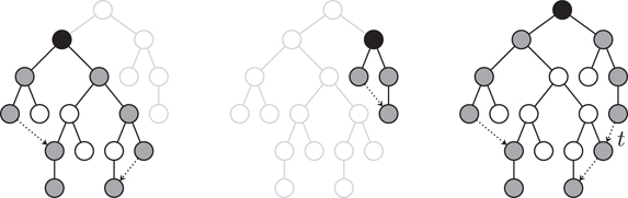
Figure 46.2Combining two subtrees and adding a new thread t.
In order to achieve linear running time it must be ensured that the contours are traversed without traversing (too many) nodes not belonging to the contours. This is achieved by introducing a thread for each leaf of the subtree that has a successor in the same contour. The thread is a pointer to this successor. See Figure 46.2 for an illustration where the threads are represented by dotted arrows. For every node of the contour, we now have a pointer to its successor in the left (right) contour given either by its leftmost (rightmost) child or by the thread. Finally, to update the threads, a new thread has to be added whenever two subtrees of different height are combined.
Once the shift has been determined for T(wright) we omit shifting the subtree by updating the coordinates of its nodes, since this would result in quadratic running time. Instead, the position of each node is only determined preliminary and the shift for T(wright) is stored at wright as the modifier mod(wright) (see [1]). Only mod(wright) and the preliminary x-coordinate prelim(v) of the parent v are adjusted by the shift of T(wright). The modifier of wright is interpreted as a value to be added to all preliminary x-coordinates in the subtree rooted at wright, except for wright itself. Thus, the coordinates of a node v in T in the final layout is its preliminary position plus the aggregated modifier modsum(v) given by the sum of all modifiers on the path from the parent of v to the root. Once all preliminary positions and modifiers have been determined the final coordinates can be easily computed by a top-down sweep.
Theorem 46.1
[Reingold and Tilford [2]] The layout algorithm for binary trees meets the aesthetic requirements (A1–A5) and can be implemented such that the running time is O(|V|).
Proof. By construction of the algorithm it is obvious that the algorithm meets (A1–A5). So it is left to show that the running time is linear in the number of nodes. Every node of T is traversed once during the postorder and the preorder traversal. So it is left to show that the time needed to traverse the contour of the two subtrees T(wleft) and T(wright) for every node v with children wleft and wright is linear in the number of nodes of T over all such traversals.
It is obviously necessary to travel down the contours of T(wleft) and T(wright) only as far as the tree with lesser height. Thus the time spent processing a vertex v in the postorder traversal is proportional to the minimum of the height of h(T(wleft)) and h(T(wright)). The running time of the postorder traversal is then given by:
The sum can be estimated as follows. Consider a node w that is part of a contour of a subtree T(wleft). When comparing the right contour of T(wleft) and the left contour of T(wright) two cases are possible. Either w is not traversed and therefore will be part of the contour of T(v) or it is traversed when comparing T(wleft) and T(wright). In the latter case, w is part of the right contour of T(wleft) and after merging T(wleft) and T(wright) the node w is not part of the right contour of T(v). Thus every node of T is traversed at most twice and the total number of comparisons is bounded by |V|.■
We do not give the full algorithm for drawing binary trees here. Instead, the layout algorithm for n-ary trees is given in full length in the next section. The methods presented there are an expansion of Reingold and Tilfords algorithm to the more general case and still proceed for binary trees as described in this section.
46.4Level Layout for n-ary Trees
A straightforward manner to draw trees of unbounded degree is to adjust the Reingold-Tilford algorithm by traversing the children of each node v from left to right, successively computing the preliminary coordinates and the modifiers.
This however violates property (A5): the subtrees are placed as close to each other as possible and small subtrees between larger ones are piled to the left; see Figure 46.3a. A simple trick to avoid this effect is to add an analogous second traversal from right to left; see Figure 46.3b, and to take average positions after that. This algorithm satisfies (A1–A5), but smaller subtrees are usually clustered then; see Figure 46.3c.

Figure 46.3Extending the Reingold-Tilford algorithm to trees of unbounded degree.
To obtain a layout where smaller subtrees are spaced out evenly between larger subtrees as for example shown in Figure 46.3d, we process the subtrees for each node v ∈ V from left to right, see Figure 46.4. In a first step, every subtree is then placed as close as possible to the right of its left subtrees. This is done similarly to the algorithm for binary trees as described in Section 46.3 by traversing the left contour of the right subtree T(wright) and the right contour of the subforest induced by the left siblings of wright.

Figure 46.4Spacing out the smaller subtrees.
Whenever two conflicting neighbors vleft and vright are detected, forcing vright to be shifted to the right by an amount of σ, we apply an appropriate shift to all smaller subtrees between the subtrees containing vleft and vright.
More precisely, let wleft and wright be the greatest distinct ancestors of vleft and vright. Notice that both wleft and wright are children of the node v that is currently processed. Let k be the number of children w1, w2, …, wk of the current root between wleft and wright plus 1. The subtrees between wleft and wright are spaced out by shifting the subtree T(wi) to the right of wleft by an amount of , for i = 1, 2, …, k. We notice that spacing out the smaller subtrees may result in subtrees that are shifted more than once. Below, the effect on the running time for computing the shifts is determined and it is shown how to obtain a linear time implementation.
It is easy to see that this approach satisfies (A1–A5) and in addition spaces out the smaller subtrees between larger subtrees evenly. In contrast to the algorithm for binary trees (see Section 46.3) nodes are not placed on integer coordinates. Instead real values are used.
Figure 46.5 gives a layout example of a 5-ary tree. The layout algorithm considers different nodes sizes.

Figure 46.5A level layout of an n-ary tree with different node sizes.
Figure 46.6 shows a layout of a PQ-tree produced by the algorithm for binary trees. A straightforward modification of the algorithm allows the application of different nodes sizes to the Q-nodes and the usage of strictly vertical edges for the children of the Q-nodes.

Figure 46.6A level layout of a PQ-tree.
The algorithm TREELAYOUT given below works as a frame that initializes modifiers, threads, and ancestors (see Section 46.4.3), before evoking the methods PREPOSITION and ADJUST. The method PREPOSITION computes the shifts and preliminary positions of the nodes.
Based on the results of the function PREPOSITION the function ADJUST given in Algorithm 46.2 computes the final coordinates by summing up the modifiers recursively.
Algorithm 46.1: TreeLayout (T)
  forall nodes v of T do
      mod(v) = thread(v) = 0;
      ancestor(v) = v;
  od
  let r be the root of T;
  PREPOSITION(r);
  ADJUST(r, −prelim(r));
Algorithm 46.2: Adjust(v, m)
   x(v) = prelim(v) + m;
   let y(v) be the level of v;
   forall children w of v do
      ADJUST(w, m + mod(v));
   od
Algorithm 46.3 presents the method PREPOSITION(v) that computes a preliminary x-coordinate for a node v. PREPOSITION is applied recursively to the children of v. After each call of PREPOSITION on a child w a function APPORTION is executed on w. The procedure APPORTION is the core of the algorithm and shifts a subtree such that it does not conflict with its left subforest. After spacing out the smaller subtrees by calling EXECUTESHIFTS, the node v is placed to the midpoint of its outermost children. The value distance prescribes the minimal distance between two nodes. If objects of different size are considered for the representation of the nodes, or if different minimal distances, that is, between subtrees, are specified, the value distance has to be modified appropriately.
Algorithm 46.3: PREPOSITION(v)
if v is a leaf then prelim(v) = 0; if v has a left sibling w then prelim(v) = prelim(w) + distance; end else let defaultAncestor be the leftmost child of v; forall children w of v from left to right do PREPOSITION(w); APPORTION(w,defaultAncestor); od EXECUTESHIFTS(v); midpoint =(prelim(leftmost child of v) + prelim(rightmost child of v)); if v has a left sibling w then prelim(v) = prelim(w) + distance; mod(v) = prelim(v)−midpoint; else prelim(v) = midpoint; end end
46.4.2Combining a Subtree and its Left Subforest
Before presenting APPORTION in detail, we need to consider efficient strategies for the different task that are performed by this function.
Similar to the threads used for binary trees (see Section 46.3), APPORTION uses threads to follow the contours of the right subtree and the left subforest. The fact that the left subforest is no tree in general does not create any additional difficulty.
One major task of APPORTION is that it has to space out the smaller subtrees between the larger ones. More precisely, if APPORTION shifts a subtree to the right to avoid a conflict with its left subforest, APPORTION has to make sure that the shifts of the smaller subtrees of the left subforest are determined.
A straightforward implementation computes the shifts for the intermediate smaller subtrees after the right subtree has been moved. However, as has been shown in Reference 5, this strategy has an aggregated runtime of Ω(|V|3/2). To prove this consider a tree Tk such that the root has k children v1, v2, …, vk (see Figure 46.7 for k = 3). The children are numbered from left to right. Except for v1 let the i-th child vi be the root of a subtree Tk(vi) that consist of a chain of i nodes. Between each pair vi, vi + 1, i = 1, 2, …, k − 1, of these children, add k children as leaves. Moreover, the subtree Tk(v1) is modified as follows. Its root v1 has 2k + 5 children, and up to level k − 1, every rightmost child of the 2k + 5 children again has 2k + 5 children. The number of nodes of Tk is

Figure 46.7T3.
When traversing the nodes v1, v2, …, vk in order to determine their shifts, the subtree chain Tk(vi) conflicts with the first subtree Tk(v1) on level i. Hence, all (i − 1)(k + 1) − 1 smaller subtrees between Tk(v1) and Tk(vi) are shifted. Thus, the total number of shifting steps is
Since the number of nodes in Tk is |V| ∈ Θ(k2), this shows that a straightforward implementation needs Ω(|V|3/2) time in total.
Let T(vi), i ∈ {2, 3, …, k} be the subtree that has to be shifted. Let vleft and vright be two neighboring nodes on some level l such that
•vleft is in the left subforest and vright is in T(vi) respectively, and
•vleft and vright determine the shift of T(vi).
In order to develop an efficient method for spacing out the smaller subtrees two tasks have to be solved.
•The tree T(vj), j ∈ {1, 2, …, i − 1}, with has to be maintained in order to determine the smaller subtrees to the left of T(vi) that have to be spaced out.
•Shifting the smaller subtrees between T(vj) and T(vi) has to be done efficiently.
The next Section 46.4.3 shows how to obtain the tree T(vj) efficiently. Section 46.4.4 gives a detailed description on how to compute the shift of T(vi). and Section 46.4.5 presents a method that spaces out smaller subtrees.
We first describe how to obtain the subtree T(vj) that contains the node vleft. The problem is equivalent to finding the greatest distinct ancestors wleft and wright of the nodes vleft and vright, where in this case wleft is equal to the root vj of the subtree that we need to determine and . It is possible to apply an algorithm by Schieber and Vishkin [24] that determines for each pair of nodes its greatest distinct ancestors in constant time, after an O(|V|) preprocessing step. Since their algorithm is somewhat tricky, and one of the greatest distinct ancestors, namely vi, is known anyway, we apply a much simpler algorithm. Furthermore, as vright is always the right neighbor of vleft, the left one of the greatest distinct ancestors only depends on vleft. Thus we may shortly call it the ancestor of vleft in the following.
To store the ancestor of a node u a pointer ancestor(u) is introduced and initialize it to u itself. The pointer ancestor(u) for any node u is not updated throughout the algorithm. Instead, a defaultAncestor is used and ancestors are only determined for the nodes u on the right contour of the left subforest during the shift of the subtree T(vi). This strategy ensures that we obtain linear running time.
We make sure that for every i = 2, 3, …, k the following property for all nodes u on the right contour of holds:
(*) If ancestor(u) is up to date, that is, u is a child of v, then ancestor(u) = wleft; otherwise, defaultAncestor is the correct ancestor(u).
For i = 2 we have that . The defaultAncestor for all nodes on the right contour is obviously v1 and therefore defaultAncestor is set equal to v1. It is easy to recognize if a node u on the right contour has a pointer ancestor(u) that is up to date: either ancestor(u)= v1, or the level l(ancestor(u)) is greater than l(v1). This obviously fulfills property (*), see Figure 46.8a for an illustration.

Figure 46.8Adjusting ancestor pointers when adding new subtrees: the pointer ancestor(u) is represented by a solid arrow if it is up to date and by a dashed arrow if it is expired. In the latter case, the defaultAncestor is used and drawn black. When adding a small subtree, all ancestor pointers ancestor(u) of its right contour are updated. When adding a large subtree, only defaultAncestor is updated.
After adding a subtree T(vi − 1) to for each i = 3, 4, …, k two cases need to be considered. If the height h(T(vi − 1)) is lesser or equal to the height of the subforest , the pointer ancestor(u) is set to vi − 1 for all nodes u on the right contour of T(vi − 1). This obviously fulfills property (*); see Figure 46.8b for an illustration. Moreover, the number of update operations is equal to the number of comparisons between the nodes on the left contour of T(vi − 1) and their neighbors in . Hence the total number of all these update operations is in O(|V|).
If the height h(T(vi − 1)) is greater than the height of , we omit updating all nodes on the right contour of T(vi − 1) in order to obtain linear running time. Instead, it suffices to set defaultAncestor to vi − 1, since either ancestor(u)= vi − 1, or l(ancestor(u)) > l(v1) holds for any node in the right contour, and all smaller subtrees in the do not contribute to the right contour anymore. Thus property (*) is fulfilled; see Figure 46.8c for an illustration.
In algorithm 46.4 the function ANCESTOR is given. It returns wleft of u as described above.
Algorithm 46.4: ANCESTOR(u,wright,defaultAncestor)
   if ancestor(u) is a sibling of wright then
      return ancestor(wright);
   else
      return defaultAncestor;
   end
To give the function APPORTION in Algorithm 46.5 a more readable annotation, we use subscripts f and o to describe the different contours of the left subforest and the right subtree. The subscript f is used for neighboring nodes on the contours that are facing each other and thus is used for the nodes on the right contour of the left subforest and the left contour of the right subtree T(vi), i = 2, 3, …, k. We use o for the left contour of and for the right contour of T(vi), describing the nodes that are on the outside of the combined subforest .
The nodes traversing the contours are vfright, vfleft, voleft, and voright, where the subscript left describes nodes of the left subforest and right nodes of the right subtree. For summing up the modifiers along the contour (see also Sect. 46.3), respective variables sfright, sfleft, soleft, and soright are used.
Whenever two nodes of the facing contours conflict, we compute the left one of the greatest distinct ancestors using the function ANCESTOR and call MOVESUBTREE to shift the subtree and prepare the shifts of smaller subtrees.
Finally, a new thread is added (if necessary) as explained in Section 46.3. Observe that we have to adjust ancestor(voright) or defaultAncestor to keep property (*). The functions NEXTLEFT and NEXTRIGHT return the next node on the left and right contour, respectively (see Algorithms 46.6 and 46.7).
46.4.5Shifting the Smaller Subtrees
For spacing out the smaller subtrees evenly, the number of the smaller subtrees between the larger ones has to be maintained. Since simply counting the number of smaller children between two larger subtrees T(vj) and T(vi), 1 ≤ j < i ≤ k would result in Ω(n3/2) time in total, it is determined as follows. The children of v are numbered consecutively. Once the pair of nodes that defines the maximum shift on T(vi) has been determined, the greatest distinct ancestors and are easily determined by the approach described in Section 46.4.3. The number i − j − 1 gives the number of in between subtrees in constant time.
In order to obtain a linear runtime, we make sure that each smaller subtree between a pair of larger ones is shifted at most once.
Thus whenever a subtree of T(vi) is considered to be placed next to the left subforest , we do not modify the shift of the smaller subtrees. Such an approach would result in quadratic runtime by the fact that smaller subtrees are shifted every time they are in between a pair of greater subtrees. Instead, a system is installed, that allows to adopt the shift of the smaller subtrees by traversing the nodes v1, v2, …, vk once after the last child vk of v has been shifted.
For every node vg, g = 1, 2, …, k, real numbers shift(vg) and change(vg) are introduced and initialized by zero. Let T(vj), 1 ≤ j < i ≤ k, be the subtree that defines the σ on the subtree T(vi). Let θ = i − j be the number of subtrees between vi and vj, plus 1. Then, for t = 1, 2, …, i − j − 1, the t-th subtree T(vj+t) has to be moved by t·σ/θ. In other words: the tree T(vj+t) is shifted by σ − (i − (j + t))·σ/θ, for example,
Algorithm 46.5: APPORTION(v,defaultAncestor)
   if v has a left sibling w then
      vrightf = vrighto = v;
      vleftf = w;
      vlefto be the leftmost sibling of vrightf;
      srightf = mod(vrightf);
      srighto = mod(vrighto);
      sleftf = mod(vleftf);
      slefto = mod(vlefto);
      while NEXTRIGHT(vleftf)≠0 and NEXTLEFT(vrightf)≠0 do
          vleftf = NEXTRIGHT(vleftf);
          vrightf = NEXTLEFT(vrightf);
          vlefto = NEXTLEFT(vlefto);
          vrighto = NEXTRIGHT(vrighto);
          ancestor(vrighto) = v;
          σ = (prelim(vleftf) + sleftf)−(prelim(vrightf) + srightf) + distance;
          if σ >0 then
              MOVESUBTREE(ANCESTOR(vleftf,v,defaultAncestor),v,σ);
              srightf = srightf + σ;
              srighto = srighto + σ;
          end
          sleftf = sleftf + mod(vleftf);
          srightf = srightf + mod(vrightf);
          slefto = slefto + mod(vlefto);
          srighto = srighto + mod(vrighto);
      end
   end
   if NEXTRIGHT(vleftf)≠0 and NEXTRIGHT(vrighto) = 0 then
      thread(vrighto) = NEXTRIGHT(vleftf);
      mod(vrighto) = mod(vrighto) + sleftf−srighto;
   end
   if NEXTLEFT(vrightf)≠0 and NEXTLEFT(vlefto) = 0 then
      thread(vlefto) = NEXTLEFT(vrightf);
      mod(vlefto) = mod(vlefto) + srightf−slefto;
      defaultAncestor = v;
   end
Algorithm 46.6: NEXTLEFT(v)
    if v has a child then
       return the leftmost child of v;
    else
       return thread(v);
    end
Algorithm 46.7: NEXTRIGHT(v)
    if v has a child then
       return the rightmost child of v;
    else
       return thread(v);
    end
•for t = i − j − 1 the subtree T(vi − 1) is shifted by σ − σ/θ,
•for t = i − j − 2 the subtree T(vi − 2) is shifted by σ − 2·σ/θ,
•and for t = 1 the subtree T(vj + 1) is shifted by σ − (i − j − 1)·σ/θ.
The shift of the subtrees T(vj + t), t = 1, 2, …, i − j − 1, depends on the shift of T(vi) and if traversed from right to left, is decreased linear by σ/θ.
Since the decrease σ/θ is linear for every pair of greater subtrees, we use a trick and aggregate the amount of shift for the intermediate smaller subtrees by storing σ in an array shift() of size k and by storing the σ/θ in an array change() of size k. The values for shifting the subtrees T(vj + t), t = 1, 2, …, i − j − 1, are then stored at vi and vj:
1.The value shift(vi) is increased by σ
2.The value change(vi) is decreased by σ/θ
3.The value change(vj) is increased by σ/θ
Figure 46.9 shows an example on setting the values of shift() and change().

Figure 46.9Aggregating the shifts: the top number at every node u indicates the value of shift(u), and the bottom number indicates the value of change(u).
By construction of the arrays shift() and change() we then obtain the shift of T(vg), g = 1, 2, …, k, (including the “original” shift of the subtree T(vi)) as follows. The children vg, g = k, k − 1, …, 1, are traversed from right to left. Two real values σ and change are maintained to store the shifts and the decreases of shift per subtree, respectively. These values are initialized with zero. When visiting child vg, g ∈ {k, k − 1, …, 1} the subtree T(vg) is shifted to the right by σ (i.e., we increase prelim(vg) and mod(vg) by σ. Furthermore, change ins increased by change(vg), and σ is increased by shift(vg) and by change(vg) and we continue with vg − 1.
It is easy to see that this algorithm shifts each subtree by the correct amount, see Figure 46.10 for an example.

Figure 46.10Executing the shifts: the third and the fourth line of numbers at a node u indicate the values of σ and change before shifting u, respectively.
The function MOVESUBTREE(wleft,wright,σ) given in algorithm 46.8 performs an update of the arrays shift() and change(). We recall that wleft and wright are the greatest distinct ancestors of vleft and vright and correspond to children vi and vj, 1 ≤ i < j ≤ k, respectively. MOVESUBTREE shifts the subtree T(wright) by increasing prelim(wright) and mod(wright) by the amount of σ. The shifts of the intermediate smaller subtrees between T(wleft) and T(wright) are prepared by adjust change(wright), shift(wright), and change(wleft).
The function EXECUTESHIFTS(v) traverses its children from right to left and determines the total shift of the children based on the arrays shift() and change().
Algorithm 46.8: MOVESUBTREE(wleft,wright, σ)
    θ = number(wright)−number(wleft);
    change(wright) = change(wright)−σ / θ;
    shift(wright) = shift(wright) + σ;
    change(wleft) = change(wleft) + σ / θ;
    prelim(wright) = prelim(wright) + σ;
    mod(wright) = mod(wright) + σ;
Algorithm 46.9: EXECUTESHIFTS
    σ = 0;
    change = 0;
    forall children w of v from right to left do
        prelim(w) = prelim(w) + σ;
        mod(w) = mod(w) + σ;
        change = change + change(w);
        σ = σ + shift(w) + change;
    od
Theorem 46.2
[Buchheim et al [5]] The layout algorithm for n-ary trees meets the aesthetic requirements (A1)–(A5), spaces out smaller subtrees evenly, and can be implemented to run in O(|V|).
Proof. By construction of the algorithm it is obvious that the algorithm meets (A1–A5) and spaces out the smaller subtrees evenly. So it is left to show that the running time is linear in the number of nodes.
Every node of T is traversed once during the traversals PREPOSITION and ADJUST. Similar reasoning as in the proof of theorem 46.1 for binary trees shows that the time needed to traverse the left contour of the subtree T(vi) and the right contour of subforest , i = 2, 3, …, k for every node v with children vi, i = 1, 2, …, k is linear in the number of nodes of T over all such traversals. Moreover, we have that by construction the number of extra operations for spacing out the smaller subtrees is linear in |V| plus the number of nodes traversed in the contours. This proofs the theorem.■
A radial layout of a tree is a variation of a level drawing, where the levels are concentric circles c1, c2, …, ch(T) around the root placed at the origin c0. Figure 46.11 shows an example of a radial layout. The radius of a circle ci, i = 1, 2, …, h(T), is given by an increasing function r(i). This type of layout is frequently used for representing a free tree. A free tree is a tree without a specific root. To layout a free tree, a node is chosen as a fictitious root that minimizes the height of the resulting subtrees. A straightforward manner to obtain a radial layout of a tree is to modify the algorithms for level drawings as presented in Sections 46.3 and 46.4.

Figure 46.11A radial layout of a binary tree.
To guarantee that the resulting drawing is planar, the subtree T(v) of each node v is drawn within an annulus wedge w(v). In order to permit edges with endpoints in w(v) to extend outside w(v) and thus to conflict with other edges, the nodes in the subtree T(v) are placed within a convex subset s(v) of w(v). Given the level l(v), the node v is placed on cl(v). Suppose that the tangent to cl(v) through v meets the points a and b on cl(v) + 1. Then s(v) is chosen to be the unbounded region that is given by the line segment ab and the rays from the root of T and the node a and b. The children vj, j = 1, 2, …, k of v are then arranged on cl(v) + 1 within s(v) according to the number of leaves in T(vj).
If the distance between consecutive circles ci, ci + 1 i = 0, 1, …, h(T) − 1, is equal, it can be easily shown that the area occupied by the layout is in
Different algorithms for the radial layout of trees have been presented by [6–8] depending on the choice of the root, the radii of the circles and the angle of the annulus wedge. Symmetry oriented algorithms have also been developed, see for example, [9].
An hv-layout of a binary tree is an upward (but not strictly upward) straight line orthogonal drawing with edges drawn as rightward horizontal or downward vertical segments. The “hv” stands for horizontal-vertical. For any vertex v in a binary tree T we either have:
1.A child of v is either
a.Aligned horizontally with v and to the right of v or
b.Vertically aligned below v.
2.The smallest rectangles that cover the area of the subtrees of the children of v in the layout do not intersect.
Figure 46.12 shows an example of a hv-layout

Figure 46.12A hv-layout of a binary tree.
A hv-layout is generated by applying a dived and conquer approach. The divide step constructs the hv-layout of the left and the right subtrees, while the conquer step either performs a horizontal or a vertical combination. Figure 46.13 shows the two types of combination.

Figure 46.13A horizontal combination (a) and a vertical combination (b).
If the left subtree a node v is placed to the left in a horizontal combination and below in a vertical combination, the layout preserves the ordering of the children of v. The height and width of such a drawing is at most |V| − 1. A straightforward way to reduce the size of a hv-drawing to a height of at most log |V| is to use only horizontal combinations and to place the larger subtree (in terms of number of nodes) to the right of the smaller subtree. This right heavy hv layout is not order preserving and can be produced in O(|V|) requiring only an area of O(|V| log |V|). The right heavy hv approach can be easily extended to draw n-ary trees as scetched in Figure 46.14.

Figure 46.14A hv-layout of a n-ary tree.
AS already presented in the introduction, this type of layout has been extensively studied for example, in References 10–21 21 to obtain results on minimal area requirements of tree layouts.
Recently Garg and Ruse [22] showed by flipping the subtrees rooted at a node v horizontally or vertically, it is possible to obtain tree layouts for binary trees with an O(|V|) area and with a pre specified aspect ratio in the range of [1, |V|α], with α ∈ [0, 1). These layouts are non upward straight line orthogonal layouts.
I gratefully acknowledge the contributions of Christoph Buchheim, who provided the figures and the implementation from our paper [5] and Merijam Percan for careful proof reading.
1.C. Wetherell and A. Shannon. Tidy drawings of trees. IEEE Trans. Softw. Eng., 5(5):514–520, 1979.
2.E. Reingold and J. Tilford. Tidier drawing of trees. IEEE Trans. Softw. Eng., SE-7(2):223–228, 1981.
3.T. Cormen, C. Leiserson, and R. Rivest. Introduction to Algorithms. MIT-Press. (1990).
4.Q. Walker, II. A node-positioning algorithm for general trees. Softw. – Pract. Exp., 20(7):685–705, 1990.
5.C. Buchheim, M. Jünger, and S. Leipert. Improving walker’s algorithm to run in linear time. In M. Goodrich, editor, Graph Drawing (Proc. GD 2002), volume 2528 of LNCS, pages 344–353. Springer-Verlag, 2002.
6.M. Bernard. On the automated drawing of graphs. In 3rd Caribbean Conference on Combinatorics and Computing, pp. 43–55, 1981.
7.P. Eades. Drawing free trees. Bulletin of the Inst. for Combinatorics and its Applications, 5:10–36, 1992.
8.C. Esposito. Graph graphics: Theory and practice. Comput. Math. Appl., 15(4):247–253, 1988.
9.J. Manning and M. Atallah. Fast detection and display of symmetry in trees. Congr. Numer., 64:159–169, 1988.
10.P. Crescenzi, G. Di Battista, and A. Piperno. A note on optimal area algorithms for upward drawings of binary trees. Comput. Geom, 2:187–200, 1992.
11.P. Crescenzi and A. Piperno. Optimal-area upward drawings of AVL trees. In R. Tamassia and I. G. Tollis, editors, Graph Drawing (Proc. GD 1994), volume 894 of LNCS, pages 307–317. Springer-Verlag, 1995.
12.S. K. Kim. Simple algorithms for orthogonal upward drawing of binary and ternary trees. In Proc. 7th Canad. Conf. Comput. Geometry, pp. 115–120, 1995.
13.S. K. Kim. H-V drawings of binary trees. In Software Visualization, volume 7 of Software Engineering and Knowledge Engineering, pages 101–116, 1996.
14.X. Lin, P. Eades, T. Lin. Minimum size h-v drawings. In Advanced Visual Interfaces, volume 36 of World Scientific Series in Computer Science, pages 386–394, 1992.
15.X. Lin, P. Eades, T. Lin. Two tree drawing conventions. Int. J. Comput. Geom. Appl., 3(2):133–153, 1993.
16.Y. Shiloach. Arrangements of Planar Graphs on the Planar Lattice. PhD thesis, Weizmann Institute of Science, 1976.
17.L. Trevisan. A note on minimum-area upward drawing of complete and Fibonacci trees. Inform. Process. Lett., 57(5):231–236, 1996.
18.P. Crescenzi, P. Penna, and A. Piperno. Linear-area upward drawings of AVL trees. Comput. Geom. Theory Appl., 9(25–42), 1998. (special issue on Graph Drawing, edited by G. Di Battista and R. Tamassia).
19.P. Crescenzi and P. Penna. Strictly-upward drawings of ordered search trees. Theor. Comput. Sci., 203(1):51–67, 1998.
20.A. Garg, M. T. Goodrich, and R. Tamassia. Planar upward tree drawings with optimal area. Int. J. Comput. Geom. Appl., 6:333–356, 1996.
21.C.-S. Shin, S. K. Kim, and K.-Y. Chwa. Area-efficient algorithms for straight-line tree drawings. Comput. Geom. Theory Appl., 15:175–202, 2000.
22.A. Garg and A. Rusu. Straight-line drawings of binary trees with linear area and arbitrary aspect ratio. In M. Goodrich, editor, Graph Drawing (Proc. GD 2002), volume 2528 of LNCS, pages 320–331. Springer-Verlag, 2002.
23.K.R. Supovit and E. Reingold. The complexity of drawing trees nicely. Act Informatica, 18:377–392, 1983.
24.B. Schieber and U. Vishkin. On finding lowest common ancestors: Simplification and parallelization. In Proceedings of the Third Aegean Workshop on Computing, volume 319 of Lecture Notes in Computer Science, pages 111–123. Springer-Verlag, 1998.
*This chapter has been reprinted from first edition of this Handbook, without any content updates.
†We have used this author’s affiliation from the first edition of this handbook, but note that this may have changed since then.