
LEDA, a Platform for Combinatorial and Geometric Computing*
Stefan Naeher
University of Trier
Ease of Use•Extensibility•Correctness•Availability and Usage
42.3Data Structures and Data Types
Basic Data Types•Numbers and Matrices•Advanced Data Types•Graph Data Structures•Geometry Kernels•Advanced Geometric Data Structures
Word Count•Shortest Paths•Curve Reconstruction•Upper Convex Hull•Delaunay Flipping•Discussion
LEDA, the Library of Efficient Data Types and Algorithms, aims at being a comprehensive software platform for the area of combinatorial and geometric computing. It provides a sizable collection of data types and algorithms in C++. This collection includes most of the data types and algorithms described in the text books of the area [1–10]. LEDA supports a broad range of applications. It has already been used in such diverse areas as code optimization, VLSI design, graph drawing, graphics, robot motion planning, traffic scheduling, geographic information systems, machine learning and computational biology.
The LEDA project was started in 1988 by Kurt Mehlhorn and Stefan Näher. The first months they spent on the specification of different data types and on selecting the implementation language. At that time the item concept came up as an abstraction of the notion “pointer into a data structure.” Items provide direct and efficient access to data and are similar to iterators in the standard template library. The item concept worked successfully for all test cases and is now used for most data types in LEDA. Concurrently with searching for the correct specifications several languages were investigated for their suitability as an implementation platform. Among the candidates were Smalltalk, Modula, Ada, Eiffel, and C++. The language had to support abstract data types and type parameters (genericity) and should be widely available. Based on the experiences with different example programs C++ was selected because of its flexibility, expressive power, and availability.
We discuss some of the general aspects of the LEDA system.
The library is easy to use. In fact, only a small fraction of the users are algorithms experts and many users are not even computer scientists. For these users the broad scope of the library, its ease of use, and the correctness and efficiency of the algorithms in the library are crucial. The LEDA manual [11] gives precise and readable specifications for the data types and algorithms mentioned above. The specifications are short (typically not more than a page), general (so as to allow several implementations) and abstract (so as to hide all details of the implementation).
Combinatorial and geometric computing is a diverse area and hence it is impossible for a library to provide ready-made solutions for all application problems. For this reason it is important that LEDA is easily extendible and can be used as a platform for further software development. In many cases LEDA programs are very close to the typical text book presentation of the underlying algorithms. The goal is the equation Algorithm + LEDA = Program.
LEDA extension packages (LEPs) extend LEDA into particular application domains and areas of algorithmics not covered by the core system. LEDA extension packages satisfy requirements, which guarantee compatibility with the LEDA philosophy. LEPs have a LEDA-style documentation, they are implemented as platform independent as possible and the installation process allows a close integration into the LEDA core library. Currently, the following LEPs are available: PQ-trees, dynamic graph algorithms, a homogeneous d-dimensional geometry kernel, and a library for graph drawing.
Programming is a notoriously error-prone task; this is even true when programming is interpreted in a narrow sense: going from a (correct) algorithm to a program. The standard way to guard against coding errors is program testing. The program is exercised on inputs for which the output is known by other means, typically as the output of an alternative program for the same task. Program testing has severe limitations. It is usually only done during the testing phase of a program. Also, it is difficult to determine the “correct” suite of test inputs. Even if appropriate test inputs are known it is usually difficult to determine the correct outputs for these inputs: alternative programs may have different input and output conventions or may be too inefficient to solve the test cases.
Given that program verification, that is, formal proof of correctness of an implementation, will not be available on a practical scale for some years to come, program checking has been proposed as an extension to testing [12,13]. The cited papers explored program checking in the area of algebraic, numerical, and combinatorial computing. In References 14–16 program checkers are presented for planarity testing and a variety of geometric tasks. LEDA uses program checkers for many of its implementations.
In computational geometry the correctness problem is even more difficult because geometric algorithms are frequently formulated under two unrealistic assumptions: computers are assumed to use exact real arithmetic (in the sense of mathematics) and inputs are assumed to be in general position. The naive use of floating point arithmetic as an approximation to exact real arithmetic very rarely leads to correct implementations. In a sequence of papers [17–21] the degeneracy and precision issues have been investigated and LEDA was extended based on this theoretical work. It now provides exact geometric kernels for two-dimensional and higher dimensional computational geometry [22] and also correct implementations for basic geometric tasks, for example, two-dimensional convex hulls, Delaunay diagrams, Voronoi diagrams, point location, line segment intersection, and higher-dimensional convex hulls and Delaunay triangulations.
An elegant (theoretical) approach to the degeneracy problem is symbolic perturbation. However, this method of forcing input data into general position can cause some serious problems in practice. In many cases, it increases the complexity of (intermediate) results considerably and furthermore, the final limit process turns out to be very difficult in particular in the presence of combinatorial structures. For this reason, LEDA follows a different approach. It copes with degeneracies directly by treating the degenerate case as the “normal” case. This approach proved to be very effective for many geometric problems.
LEDA is realized in C++ and can be used on many different platforms with many different compilers. LEDA is now used at many academic sites. A commercial version of LEDA is marketed by Algorithmic Solutions Software GmbH (<www.algorithmic-solutions.com>).
LEDA uses templates for the implementation of parameterized data types and for generic algorithms. However, it is not a pure template library and therefore is based on a number of object code libraries of precompiled code. Programs using LEDA data types or algorithms have to include the appropriate LEDA header files into their source code and have to be linked with one or more of these libraries. The four object code libraries are built on top of each other. Here, we only give a short overview. Consult the LEDA user manual [11] or the LEDA book [23] for a detailed description.
•The Basic Library (libL) contains system dependent code, basic data structures, numbers and types for linear algebra, dictionaries, priority queues, partitions, and many more basic data structures and algorithms.
•The Graph Library (libG) contains different types of graphs and a large collection of graph and network algorithms
•The 2D Geometry Library (libP) contains the two-dimensional geometric kernels advanced geometric data structures, and a large number of algorithms for two-dimensional geometric problems.
•The 3D Geometry Library (libP) contains the three-dimensional kernels and some algorithms for three-dimensional problems.
•The Window Library(libW) supports graphical output and user interaction for both the X11 platform (Unix) and Microsoft Windows systems. It also contains animation support: GraphWin, a powerful graph editor, and GeoWin, a interactive tool for the visualization of geometric algorithms. See Section 42.5 for details.
42.3Data Structures and Data Types
LEDA contains a large number of data structures from the different areas of combinatorial and geometric computing. However, as indicated in the name of the library, LEDA was not designed as a collection of data structures but as a library of (parameterized) data types. For each (abstract) data type in the library there is at least one data structure which implements this type. This separation of specification (by an abstract data type) and implementation (by an actual data structure) is crucial for a software component library. It allows to change the underlying implementation or to choose between different implementations without having to change the application program. In general, there is one default data structure for each of the advanced data types, for example, avl-trees for dictionaries, skiplists for sorted sequences, binary heaps for priority queues, and a union-find structure for partitions. For most of these data types a number of additional data structures are available and can be specified by an optional template argument. For instance dictionary<string,int,skiplist> specifies a dictionary type with key type string and information type int which is implemented by the skiplist data structure (see Reference 23 for more details and Section 42.6.1 for an example).
Of course, LEDA contains a complete collection of all basic data types, such as strings, stacks, queues, lists, arrays, tuples …which are ubiquitous in all areas of computing.
Numbers are at the origin of computing. We all learn about integers, rationals, and real numbers during our education. Unfortunately, the number types int, float, and double provided by C++ are only crude approximations of their mathematical counterparts: there are only finitely many numbers of each type and for floats and doubles the arithmetic incurs rounding errors. LEDA offers the additional number types integer, rational, bigfloat, and real. The first two are the exact realization of the corresponding mathematical types and the latter two are better approximations of the real numbers. Vectors and matrices are one- and two-dimensional arrays of numbers, respectively. They provide the basic operations of linear algebra.
A collection of parameterized data types representing sets, partitions, dictionaries, priority queues, sorted sequences, partitions and sparse arrays (maps, dictionary and hashing arrays). Type parameters include the key, information, priority, or element type and (optional) the data structure used for the implementation of the type. The list of data structures includes skiplists (see Chapter 14), (a, b)-trees, avl-trees, red-black trees, bb[α]-trees (see Chapter 11), randomized search trees (see Chapter 14), Fibonacci-heaps, binary heaps, pairing heaps (see Chapter 7), redistributive heaps, union find with path compression (Chapter 34), dynamic perfect hashing, cuckoo hashing (see Chapter 9), Emde-Boas trees, …. This list of data structures is continuously growing and adapted to new results from the area for data structures and algorithms.
The graph data type (Chapter 4) is one of the central data types in LEDA. It offers the standard iterations such as “for all nodes v of a graph G do” (written forall_nodes(v, G)) or “for all edges e incident to a node v do” (written forall_out_edges(e, v)), it allows to add and delete vertices and edges and it offers arrays and matrices indexed by nodes and edges, (see Reference 23 Chapter 6 for details and Section 42.6.2 for an example program). The data type graph allows to write programs for graph problems in a form very close to the typical text book presentation.
LEDA offers kernels for two- and three-dimensional geometry, a kernel of arbitrary dimension is available as an extension package. In either case there exists a version of the kernel based on floating point Cartesian coordinates (called float-kernel) as well as a kernel based on rational homogeneous coordinates (called rat-kernel). All kernels provide a complete collection of geometric objects (points, segments, rays, lines, circles, simplices, polygons, planes, etc.) together with a large set of geometric primitives and predicates (orientation of points, side-of-circle tests, side-of-hyperplane, intersection tests and computation, etc.). For a detailed discussion and the precise specification see Chapter 9 of the LEDA book [23]. Note that only for the rational kernel, which is based on exact arithmetic and floating-point filters, all operations and primitives are guaranteed to compute the correct result.
42.3.6Advanced Geometric Data Structures
In addition to the basic kernel data structures LEDA provides many advanced data types for computational geometry. Examples are
•A general polygon type (gen_polygon or rat_gen_polygon) with a complete set of boolean operations. Its implementation is based on an efficient and robust plane sweep algorithms for the construction of the arrangement of a set of straight line segments (see References 23 and 24 Chapter 11.7 for a detailed description).
•Two- and higher-dimensional geometric tree structures, such as range, segment, interval and priority search trees (see Chapter 19).
•Partially and fully persistent search trees (Chapter 33).
•Different kinds of geometric graphs (triangulations, Voronoi diagrams, and arrangements)
•A dynamic point_set data type supporting update, search, closest point, and different types of range query operations on one single representation which is based on a dynamic Delaunay triangulation (see Reference 23 Chapter 11.6).
The LEDA project had never the goal to provide a complete collection of all algorithms. LEDA was designed and implemented to establish a platform for combinatorial and geometric computing enabling programmers to implement these algorithms themselves more easily and customized to their particular needs. But of course the library already contains a considerable number of standard algorithms.
Here we give a brief overview and refer the reader to the user manual for precise specifications and to Chapter 10 of the LEDA-book [23] for a detailed description and analysis of the corresponding implementations. In the current version LEDA offers different implementation of algorithms for the following problems:
•Sorting and searching
•Basic graph properties
•Graph traversals
•Different kinds of connected components
•Planarity test and embeddings
•Minimum spanning trees
•Shortest paths
•Network flows
•Maximum weight and cardinality matchings
•Graph drawing
•Convex hulls (also three-dimensional)
•Half-plane intersections
•(Constraint) triangulations
•Closest and farthest Delaunay and Voronoi diagrams
•Euclidean minimum spanning trees
•Closest pairs
•Boolean operations on generalized polygons
•Segment intersection and construction of line arrangements
•Minkowski sums and differences
•Nearest neighbors and closest points
•Minimum enclosing circles and annuli
•Curve reconstruction
Visualization and animation of programs is very important for the understanding, presentation, and debugging of algorithms (see Chapter 45). LEDA provides two powerful tools for interactive visualization and animation of data structures and algorithms:
The GraphWin data type (see Reference 23, Chapter 12) combines the graph and the window data type. An object of type GraphWin (short: a GraphWin) is a window, a graph, and a drawing of the graph, all at once. The graph and its drawing can be modified either by mouse operations or by running a graph algorithm on the graph. The GraphWin data type can be used to:
•Construct and display graphs,
•Visualize graphs and the results of graph algorithms,
•Write interactive demos for graph algorithms,
•Animate graph algorithms.
All demos and animations of graph algorithms in LEDA are based on GraphWin, many of the drawings in the LEDA book [23] have been made with GraphWin, and many of the geometry demos in LEDA have a GraphWin button that allows us to view the graph structure underlying a geometric object.
GraphWin can easily be used in programs for constructing, displaying and manipulating graphs and for animating and debugging graph algorithms. It offers both a programming and an interactive interface, most applications use both of them. Figure 42.1 shows a screenshot of a typical GraphWin window.
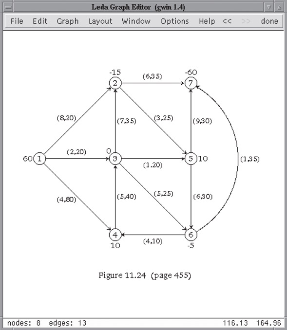
Figure 42.1A GraphWin. The display part of the window shows a graph G and the panel part of the window features the default menu of a GraphWin. G can be edited interactively, e.g., nodes and edges can be added, deleted, and moved around. It is also possible to run graph algorithms on G and to display their result or to animate their execution.
GeoWin [25] is a generic tool for the interactive visualization of geometric algorithms. GeoWin is implemented as a C++ data type. It provides support for a number of programming techniques which have shown to be very useful for the visualization and animation of algorithms. The animations use smooth transitions to show the result of geometric algorithms on dynamic user-manipulated input objects, for example, the Voronoi diagram of a set of moving points or the result of a sweep algorithm that is controlled by dragging the sweep line with the mouse (see Figure 42.2).
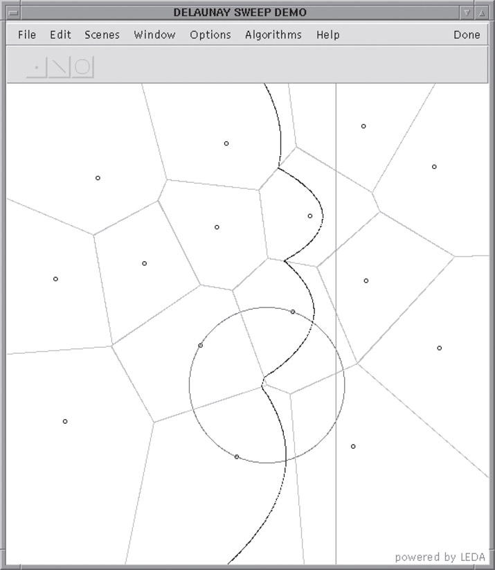
Figure 42.2GeoWin animating Fortune’s Sweep Algorithm.
A GeoWin maintains one or more geometric scenes. A geometric scene is a collection of geometric objects of the same type. A collection is simply either a standard C++-list (STL-list) or a LEDA-list of objects. GeoWin requires that the objects provide a certain functionality, such as stream input and output, basic geometric transformations, drawing and input in a LEDA window. A precise definition of the required operations can be found in the manual pages [11]. GeoWin can be used for any collection of basic geometric objects (geometry kernel) fulfilling these requirements.
The visualization of a scene is controlled by a number of attributes, such as color, line width, line style, etc. A scene can be subject to user interaction and it may be defined from other scenes by means of an algorithm (a C++ function). In the latter case the scene (also called result scene) may be recomputed whenever one of the scenes on which it depends is modified. There are three main modes for re-computation: user-driven, continuous, and event-driven.
GeoWin has both an interactive and a programming interface. The interactive interface supports the interactive manipulation of input scenes, the change of geometric attributes, and the selection of scenes for visualization.
In this section we give several programming examples showing how LEDA can be used to implement combinatorial and geometric algorithms in a very elegant and readable way. In each case we will first state the algorithm and then show the program. It is not essential to understand the algorithms in full detail; our goal is to show:
•How easily the algorithms are transferred into programs and
•How natural and elegant the programs are.
In other words, Algorithm + LEDA = Program.
We start with a very simple program. The task is to read a sequence of strings from standard input, to count the number of occurrences of each string in the input, and to print a list of all occurring strings together with their frequencies on standard output.
The program uses the LEDA types string and d_array (dictionary arrays). The parameterized data type d_array < I, E > realizes arrays with index type I and element type E. We use it with index type string and element type int.
#include <LEDA/d_array.h>#include <LEDA/impl/skiplist.h>int main(){ d_array<string,int,skiplist> N(0);string s;while (cin >> s) N[s]++;forall_defined(s,N) cout << s << " " << N[s] << endl;}
We give some more explanations. The program starts with the include statement for dictionary arrays and skiplists. In the first line of the main program we define a dictionary array N with index type string, element type int and implementation skiplist and initialize all entries of the array to zero. Conceptually, this creates an infinite array with one entry for each conceivable string and sets all entries to zero; the implementation of d_arrays stores the non-zero entries in a balanced search tree with key type string. In the second line we define a string s. The while-loop does most of the work. We read strings from the standard input until the end of the input stream is reached. For every string s we increment the entry N[s] of the array N by one. The iteration forall_defined(s, N) in the last line successively assigns all strings to s for which the corresponding entry of N was touched during execution. For each such string, the string and its frequency are printed on the standard output.
Dijkstra’s shortest path algorithm [26] takes a directed graph G = (V, E), a node s ∈ V, called the source, and a non-negative cost function on the edges cost : E → R≥0. It computes for each node v ∈ V the distance from s, see Figure 42.3. A typical text book presentation of the algorithm is as follows:
forall nodes v do
    set dist(v) to infinity.
    declare v unreached.
od
set dist(s) to 0.

while there is an unreached node do
    let u be an unreached node with minimal dist-value. (*)
    declare u reached.
    forall edges e = (u, v) out of u do
       set dist(v) = min(dist(v), dist(u) + cost(e)).
    od
od
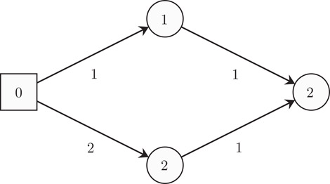
Figure 42.3A shortest path in a graph. Each edge has a non-negative cost. The cost of a path is the sum of the cost of its edges. The source node s is indicated as a square. For each node the length of the shortest path from s is shown.
The text book presentation will then continue to discuss the implementation of line (*). It will state that the pairs {(v, dist(v));v unreached} should be stored in a priority queue, for example, a Fibonacci heap, because this will allow the selection of an unreached node with minimal distance value in logarithmic time. It will probably refer to some other chapter of the book for a discussion of priority queues.
We next give the corresponding LEDA program; it is very similar to the pseudo-code above. In fact, after some experience with LEDA you should be able to turn the pseudo-code into code within a few minutes.
#include <LEDA/graph.h>#include <LEDA/node_pq.h>void DIJKSTRA(const graph& G, node s, const edge_array<double>& cost,node_array<double>& dist){ node_pq<double> PQ(G);node v;dist[s] = 0;forall_nodes(v,G){ if (v != s) dist[v] = MAXDOUBLE;PQ.insert(v,dist[v]);}while (!PQ.empty()) {node u = PQ.del_min();edge e;forall_out_edges(e,u) {v = target(e);double c = dist[u] + cost[e];if (c < dist[v]) {PQ.decrease_p(v,c);dist[v] = c;}}}}
We start by including the graph and the node priority queue data types. The function DIJKSTRA takes a graph G, a node s, an edge_array cost, and a node_array dist. Edge arrays and node arrays are arrays indexed by edges and nodes, respectively. We declare a priority queue PQ for the nodes of graph G. It stores pairs (v, dist[v]) and is initially empty. The forall_nodes-loop initializes dist and PQ. In the main loop we repeatedly select a pair (u, dist[u]) with minimal distance value and then iterate over all out-going edges to update distance values of neighboring vertices.
We next incorporate the shortest path program into a small demo. We generate a random graph with n nodes and m edges and choose the edge costs as random number in the range [0, 100]. We call the function above and report the running time.
int main(){ int n = read_int("number of nodes = ");int m = read_int("number of edges = ");graph G;random_graph(G,n,m);edge_array<double> cost(G);node_array<double> dist(G);edge e;forall_edges(e,G) cost[e] = rand_int(0,100);float T = used_time();DIJKSTRA(G,G.first_node(),cost,dist);cout << "The computation took" << used_time(T) << "seconds." << endl;}
On a graph with 10,000 nodes and 100,000 edges the computation takes less than a second.
The reconstruction of a curve from a set of sample points is an important problem in computer vision. Amenta, Bern, and Eppstein [27] introduced a reconstruction algorithm which they called CRUST. Figure 42.4 shows a point set and the curves reconstructed by their algorithm. The algorithm CRUST takes a list S of points and returns a graph G. CRUST makes use of Delaunay diagrams and Voronoi diagrams and proceeds in three steps:
•It first constructs the Voronoi diagram VD of the points in S.
•It then constructs a set L = S ∪ V, where V is the set of vertices of VD.
•Finally, it constructs the Delaunay triangulation DT of L and makes G the graph of all edges of DT that connect points in S.
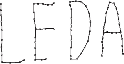
Figure 42.4A set of points in the plane and the curve reconstructed by CRUST. The figure was generated by the program presented in Section 42.6.3.
The algorithm is very simple to implement
#include <LEDA/graph.h>#include <LEDA/map.h>#include <LEDA/float_kernel.h>#include <LEDA/geo_alg.h>void CRUST(const list<point>& S, GRAPH<point,int>& G){list<point> L = S;GRAPH<circle,point> VD;VORONOI(L,VD);// add Voronoi vertices and mark themmap<point,bool> voronoi_vertex(false);node v;forall_nodes(v,VD){ if (VD.outdeg(v) < 2) continue;point p = VD[v].center();voronoi_vertex[p] = true;L.append(p);}DELAUNAY_TRIANG(L,G);forall_nodes(v,G)if (voronoi_vertex[G[v]]) G.del_node(v);}
We give some explanations. We start by including graphs, maps, the floating point geometry kernel, and the geometry algorithms. In CRUST we first make a copy of S in L. Next we compute the Voronoi diagram VD of the points in L. In LEDA we represent Voronoi diagrams by graphs whose nodes are labeled with circles. A node v is labeled by a circle passing through the defining sites of the vertex. In particular, VD[v].center() is the position of the node v in the plane. Having computed VD we iterate over all nodes of VD and add all finite vertices (a Voronoi diagram also has nodes at infinity, they have degree one in our graph representation of Voronoi diagrams) to L. We also mark all added points as vertices of the Voronoi diagram. Next we compute the Delaunay triangulation of the extended point set in G. Having computed the Delaunay triangulation, we collect all nodes of G that correspond to vertices of the Voronoi diagram in a list vlist and delete all nodes in vlist from G. The resulting graph is the result of the reconstruction.
We next incorporate CRUST into a small demo which illustrates its speed. We generate n random points in the plane and construct their crust. We are aware that it does really make sense to apply CRUST to a random set of points, but the goal of the demo is to illustrate the running time.
int main(){ int n = read_int("number of points = ");list<point> S;random_points_in_unit_square(n,S);GRAPH<point,int> G;float T = used_time();CRUST(S,G);cout << "The crust computation took" << used_time(T) << "seconds.";cout << endl;}
For 3000 points the computation takes less than a second. We can now use the preceding program for a small interactive demo.
#include <LEDA/window.h>int main(){ window W;W.display();W.set_node_width(2);W.set_line_width(2);point p;list<point> S;GRAPH<point,int> G;while (W >> p){ S.append(p);CRUST(S,G);W.clear();node v;forall_nodes(v,G) W.draw_node(G[v]);edge e;forall_edges(e,G) W.draw_segment(G[source(e)], G[target(e)]);}}
We give some more explanations. We start by including the window type. In the main program we define a window and open its display. A window will pop up. We state that we want nodes and edges to be drawn with width two. We define the list S and the graph G required for CRUST. In each iteration of the while-loop we read a point in W (each click of the left mouse button enters a point), append it to S and compute the crust of S in G. We then draw G by drawing its vertices and its edges. Each edge is drawn as a line segment connecting its endpoints. Figure 42.4 was generated with the program above.
In the next example we show how to use LEDA for computing the upper convex hull of a given set of points. The following function UPPER_HULL takes a list L of rational points (type rat_point) as input and returns the list of points of the upper convex hull of L in clockwise ordering. The algorithm is a variant of Graham’s Scan [28]. First we sort L according to the lexicographic ordering of the Cartesian coordinates and remove multiple points. If the list contains not more than two points after this step we stop. Before starting the actual Graham Scan we first skip all initial points lying on or below the line connecting the two extreme points. Then we scan the remaining points from left to right and maintain the upper hull of all points seen so far in a list called hull. Note however that the last point of the hull is not stored in this list but in a separate variable p. This makes it easier to access the last two hull points as required by the algorithm. Note also that we use the rightmost point as a sentinel avoiding the special case that hull becomes empty.
using namespace leda;list<rat_point> UPPER_HULL(list<rat_point> L){ L.sort();L.unique();if (L.length() <= 2) return L;rat_point p_min = L.front(); // leftmost pointrat_point p_max = L.back(); // rightmost pointlist<rat_point> hull;hull.append(p_max); // use rightmost point as sentinelhull.append(p_min); // first hull point// goto first point p above (p_min,p_max)while (!L.empty() && !left_turn(p_min,p_max,L.front()) L.pop();if (L.empty()) return hull;rat_point p = L.pop(); // second (potential) hull pointrat_point q;forall(q,L){ while (!right_turn(hull.back(),p,q)) p = hull.pop_back();hull.append(p);p = q;}hull.append(p); // add last hull pointhull.pop(); // remove sentinelreturn hull;}
LEDA represents triangulations by bidirected plane graphs (from the graph library) whose nodes are labeled with points and whose edges may carry additional information, for example, integer flags indicating the type of edge (hull edge, triangulation edge, etc.). All edges incident to a node v are ordered in counter-clockwise ordering and every edge has a reversal edge. In this way the faces of the graph represent the triangles of the triangulation. The graph type offers methods for iterating over the nodes, edges, and adjacency lists of the graph. In the case of plane graphs there are also operations for retrieving the reverse edge and for iterating over the edges of a face. Furthermore, edges can be moved to new nodes. This graph operation is used in the following program to implement edge flips.
Function DELAUNAY_FLIPPING takes as input an arbitrary triangulation and turns into a Delaunay triangulation by the well-known flipping algorithm. This algorithm performs a sequence of local transformations as shown in Figure 42.5 to establish the Delaunay property: for every triangle the circumscribing sphere does not contain any vertex of the triangulation in its interior. The test whether an edge has to be flipped or not can be realized by a so-called side_of_circle test. This test takes four points a, b, c, d and decides on which side of the oriented circle through the first three points a, b, and c the last point d lies. The result is positive or negative if d lies on the left or on the right side of the circle, respectively, and the result is zero if all four points lie on one common circle. The algorithms uses a list of candidates which might have to be flipped (initially all edges). After a flip the four edges of the corresponding quadrilateral are pushed onto this candidate list. Note that G[v] returns the position of node v in the triangulation graph G. A detailed description of the algorithm and its implementation can be found in the LEDA book ([23]).
void DELAUNAY_FLIPPING(GRAPH<POINT,int>& G){list<edge> S = G.all_edges();while ( !S.empty() ){ edge e = S.pop();edge r = G.rev_edge(e);// e1,e2,e3,e4: edges of quadrilateral with diagonal eedge e1 = G.face_cycle_succ(r);edge e2 = G.face_cycle_succ(e1);edge e3 = G.face_cycle_succ(e);edge e4 = G.face_cycle_succ(e3);// a,b,c,d: corners of quadrilateralPOINT a = G[G.source(e1)];POINT b = G[G.target(e1)];POINT c = G[G.source(e3)];POINT d = G[G.target(e3)];if (side_of_circle(a,b,c,d) > 0){ S.push(e1); S.push(e2); S.push(e3); S.push(e4);// flip diagonalG.move_edge(e,e2,source(e4));G.move_edge(r,e4,source(e2));}}}
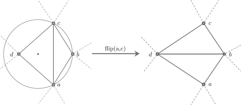
Figure 42.5Delaunay Flipping.
In each of the above examples only a few lines of code were necessary to achieve complex functionality and, moreover, the code is elegant and readable. The data structures and algorithms in LEDA are efficient. For example, the computation of shortest paths in a graph with 10,000 nodes and 100,000 edges and the computation of the crust of 5000 points takes less than a second each. We conclude that LEDA is ideally suited for rapid prototyping as summarized in the equation
Algorithm + LEDA = Efficient Program.
A large number academic and industrial projects from almost every area of combinatorial and geometric computing have been enabled by LEDA. Examples are graph drawing, algorithm visualization, geographic information systems, location problems, visibility algorithms, DNA sequencing, dynamic graph algorithms, map labeling, covering problems, railway optimization, route planning and many more. A detailed list of academic LEDA projects can be found on <http://www.mpi-sb.mpg.de/LEDA/friends> and a selection of industrial projects is shown on <http://www.algorithmic-solutions.com/enreferenzen.htm>.
1.A. V. Aho, J. E. Hopcroft and J. D. Ullman, The Design and Analysis of Computer Algorithms, Addison-Wesley, Longman Publishing Co., Inc. Boston, MA, 1974.
2.T. H. Cormen and C. E. Leiserson and R. L. Rivest, Introduction to Algorithms, MIT Press/McGraw-Hill Book Company, 1990.
3.J. H. Kingston, Algorithms and Data Structures, Addison-Wesley, 1990.
4.K. Mehlhorn, Data Structures and Algorithms 1,2, and 3, Springer, 1984.
5.J. Nievergelt and K.H. Hinrichs, Algorithms and Data Structures, Prentice Hall, 1993.
6.J. O’Rourke, Computational Geometry in C, Cambridge University Press, 1994.
7.R. Sedgewick, Algorithms, Addison-Wesley, 1991.
8.R. E. Tarjan, Data Structures and Network Algorithms, CBMS-NSF Regional Conference Series in Applied Mathematics 44, 1983.
9.C. J. van Wyk, Data Structures and C Programs, Addison-Wesley, 1988.
10.D. Wood, Data Structures, Algorithms, and Performance, Addison-Wesley, 1993.
11.K. Mehlhorn, S. Näher, M. Seel and C. Uhrig, The LEDA User Manual, Technical Report, Max-Planck-Institut für Informatik, 1999.
12.M. Blum, M. Luby and R. Rubinfeld, Self-Testing/Correcting with Applications to Numerical Problems, Proceedings of the 22nd Annual ACM Symposium on Theory of Computing (STOC90), 73–83, 1990.
13.M. Blum and S. Kannan, Designing Programs That Check Their Work, Proceedings of the 21th Annual ACM Symposium on Theory of Computing (STOC89), 86–97, 1989.
14.C. Hundack, K. Mehlhorn and S. Näher, A simple linear time algorithm for identifying Kuratowski subgraphs of non-planar graphs, unpublished manuscript, 1996.
15.K. Mehlhorn and P. Mutzel, On the Embedding Phase of the Hopcroft and Tarjan Planarity Testing Algorithm, Algorithmica, Vol. 16, No. 2, 233–242, 1995.
16.K. Mehlhorn, S. Näher, M. Seel, R. Seidel, T. Schilz, S. Schirra and C. Uhrig, Checking Geometric Programs or Verification of Geometric Structures, Computational Geometry: Theory and Applications, Vol. 12, No. 1–2, 85–103, 1999.
17.C. Burnikel, K. Mehlhorn and S. Schirra, How to compute the Voronoi diagram of line Segments: Theoretical and experimental results, Proceedings of the 2nd Annual European Symposium on Algorithms (ESA94), Lecture Notes in Computer Science 855, 227–239, 1994.
18.K. Mehlhorn and S. Näher, The Implementation of Geometric Algorithms, Proceedings of the 13th IFIP World Computer Congress, 223–231, Elsevier Science B.V. North-Holland, Amsterdam, 1994.
19.M. Seel, Eine Implementierung abstrakter Voronoidiagramme, Diplomarbeit, Fachbereich Informatik, Universität des Saarlandes, Saarbrücken, 1994.
20.C. Burnikel, K. Mehlhorn and S. Schirra, On Degeneracy in Geometric Computations, Proceedings of the 5th ACM-SIAM Sympos. Discrete Algorithms, 16–23, 1994.
21.A. Fabri, G.-J. Giezeman, L. Kettner, S. Schirra and S. Schönherr, On the Design of CGAL a Computational Geometry Algorithms Library, Software – Practice and Experience, Vol. 30, No. 11, 1167–1202, 2000.
22.Mehlhorn, K., M. Müller, S. Näher, S. Schirra, M. Seel, C. Uhrig and J. Ziegler, A Computational Basis for Higher-Dimensional Computational Geometry and Applications, Computational Geometry: Theory and Applications, Vol. 10, No. 4, 289–303, 1998.
23.K. Mehlhorn and S. Näher, LEDA: A Platform for Combinatorial and Geometric Computing, Cambridge University Press, 2000.
24.K. Mehlhorn and S. Näher, Implementation of a sweep line algorithm for the straight line segment intersection problem, Technical Report, Max-Planck-Institut für Informatik, MPI-I-94-160, 1994.
25.M. Bäsken and S. Näher, GeoWin—A Generic Tool for Interactive Visualization of Geometric Algorithms, Software Visualization, LNCS, Vol. 2269, 88–100, 2002.
26.E. W. Dijkstra, A Note on Two Problems in Connection With Graphs, Num. Math., Vol. 1, 269–271, 1959.
27.N. Amenta, M. Bern and D. Eppstein, The Crust and the beta-Skeleton: Combinatorial Curve Reconstruction, Graphical Models and Image Processing, Vol. 60, 125–135, 1998.
28.R. L. Graham, An Efficient Algorithm for Determining the Convex Hulls of a Finite Point Set, Information Processing Letters, Vol. 1, 132–133, 1972.
*This chapter has been reprinted from first edition of this Handbook, without any content updates.