
Sartaj Sahni
University of Florida
29.3Keys with Different Length
29.5Space Required and Alternative Node Structures
29.8Prefix Search and Applications
Compressed Tries with Digit Numbers•Compressed Tries with Skip Fields•Compressed Tries with Edge Information•Space Required by a Compressed Trie
Searching•Inserting an Element•Removing an Element
A trie (pronounced “try” and derived from the word retrieval) is a data structure that uses the digits in the keys to organize and search the dictionary. Although, in practice, we can use any radix to decompose the keys into digits, in our examples, we shall choose our radixes so that the digits are natural entities such as decimal digits (0, 1, 2, 3, 4, 5, 6, 7, 8, 9) and letters of the English alphabet (a–z, A–Z).
Suppose that the elements in our dictionary are student records that contain fields such as student name, major, date of birth, and social security number (SS#). The key field is the social security number, which is a nine digit decimal number. To keep the example manageable, assume that the dictionary has only five elements. Table 29.1 shows the name and SS# fields for each of the five elements in our dictionary.
Table 29.1Five Elements (Student Records) in a Dictionary
|
Name |
Social Security Number (SS#) |
|
Jack |
951-94-1654 |
|
Jill |
562-44-2169 |
|
Bill |
271-16-3624 |
|
Kathy |
278-49-1515 |
|
April |
951-23-7625 |
To obtain a trie representation for these five elements, we first select a radix that will be used to decompose each key into digits. If we use the radix 10, the decomposed digits are just the decimal digits shown in Table 29.1. We shall examine the digits of the key field (i.e., SS#) from left to right. Using the first digit of the SS#, we partition the elements into three groups–elements whose SS# begins with 2 (i.e., Bill and Kathy), those that begin with 5 (i.e., Jill), and those that begin with 9 (i.e., April and Jack). Groups with more than one element are partitioned using the next digit in the key. This partitioning process is continued until every group has exactly one element in it.
The partitioning process described above naturally results in a tree structure that has 10-way branching as is shown in Figure 29.1. The tree employs two types of nodes–branch nodes and element nodes. Each branch node has 10 children (or pointer/reference) fields. These fields, child[0:9], have been labeled 0,1, …, 9 for the root node of Figure 29.1. root.child[i] points to the root of a subtrie that contains all elements whose first digit is i. In Figure 29.1, nodes A, B, D, E, F, and I are branch nodes. The remaining nodes, nodes C, G, H, J, and K are element nodes. Each element node contains exactly one element of the dictionary. In Figure 29.1, only the key field of each element is shown in the element nodes.

Figure 29.1Trie for the elements of Table 29.1.
To search a trie for an element with a given key, we start at the root and follow a path down the trie until we either fall off the trie (i.e., we follow a null pointer in a branch node) or we reach an element node. The path we follow is determined by the digits of the search key. Consider the trie of Figure 29.1. Suppose we are to search for an element with key 951-23-7625. We use the first digit, 9, in the key to move from the root node A to the node A.child[9] = D. Since D is a branch node, we use the next digit, 5, of the key to move further down the trie. The node we reach is D.child[5] = F. To move to the next level of the trie, we use the next digit, 1, of the key. This move gets us to the node F.child[1] = I. Once again, we are at a branch node and must move further down the trie. For this move, we use the next digit, 2, of the key, and we reach the element node I.child[2] = J. When an element node is reached, we compare the search key and the key of the element in the reached element node. Performing this comparison at node J, we get a match. The element in node J, is to be returned as the result of the search.
When searching the trie of Figure 29.1 for an element with key 951-23-1669, we follow the same path as for the key 951-23-7625. The key comparison made at node J tells us that the trie has no element with key 951-23-1669, and the search returns the value null.
To search for the element with key 562-44-2169, we begin at the root A and use the first digit, 5, of the search key to reach the element node A.child[5] = C. The key of the element in node C is compared with the search key. Since the two keys agree, the element in node C is returned.
When searching for an element with key 273-11-1341, we follow the path A, A.child[2] = B, B.child[7] = E, E.child[3] = null. Since we fall off the trie, we know that the trie contains no element whose key is 273-11-1341.
When analyzing the complexity of trie operations, we make the assumption that we can obtain the next digit of a key in O(1) time. Under this assumption, we can search a trie for an element with a d digit key in O(d) time.
29.3Keys with Different Length
In the example of Figure 29.1, all keys have the same number of digits (i.e., 9). In many applications, however, different keys have different length. This does not pose a problem unless one key is a prefix of another (e.g., 27 is a prefix of 276). For applications in which one key may be a prefix of another, we normally add a special digit (say #) at the end of each key. Doing this ensures that no key is a prefix of another.
To see why we cannot permit a key that is a prefix of another key, consider the example of Figure 29.1. Suppose we are to search for an element with the key 27. Using the search strategy just described, we reach the branch node E. What do we do now? There is no next digit in the search key that can be used to reach the terminating condition (i.e., you either fall off the trie or reach an element node) for downward moves. To resolve this problem, we add the special digit # at the end of each key and also increase the number of children fields in an element node by one. The additional child field is used when the next digit equals #.
An alternative to adding a special digit at the end of each key is to give each node a data field that is used to store the element (if any) whose key exhausts at that node. So, for example, the element whose key is 27 can be stored in node E of Figure 29.1. When this alternative is used, the search strategy is modified so that when the digits of the search key are exhausted, we examine the data field of the reached node. If this data field is empty, we have no element whose key equals the search key. Otherwise, the desired element is in this data field.
It is important to note that in applications that have different length keys with the property that no key is a prefix of another, neither of just mentioned strategies is needed; the scheme described in Section 29.2 works as is.
In the worst case, a root-node to element-node path has a branch node for every digit in a key. Therefore, the height* of a trie is at most number of digits + 1.
A trie for social security numbers has a height that is at most 10. If we assume that it takes the same time to move down one level of a trie as it does to move down one level of a binary search tree, then with at most 10 moves we can search a social-security trie. With this many moves, we can search a binary search tree that has at most 210 − 1 = 1023 elements. This means that, we expect searches in the social security trie to be faster than searches in a binary search tree (for student records) whenever the number of student records is more than 1023. The breakeven point will actually be less than 1023 because we will normally not be able to construct full or complete binary search trees for our element collection.
Since a SS# is nine digits, a social security trie can have up to 109 elements in it. An AVL tree with 109 elements can have a height that is as much as (approximately) 1.44 log2(109 + 2) = 44. Therefore, it could take us four times as much time to search for elements when we organize our student-record dictionary as an AVL tree than when this dictionary is organized as a trie!
29.5Space Required and Alternative Node Structures
The use of branch nodes that have as many child fields as the radix of the digits (or one more than this radix when different keys may have different length) results in a fast search algorithm. However, this node structure is often wasteful of space because many of the child fields are null. A radix r trie for d digit keys requires O(rdn) child fields, where n is the number of elements in the trie. To see this, notice that in a d digit trie with n information nodes, each information node may have at most d ancestors, each of which is a branch node. Therefore, the number of branch nodes is at most dn. (Actually, we cannot have this many branch nodes, because the information nodes have common ancestors like the root node.)
We can reduce the space requirements, at the expense of increased search time, by changing the node structure. For example, each branch node of a trie could be replaced by any of the following:
1.A chain of nodes, each node having the three fields digit Value, child, next. Node A of Figure 29.1, for example, would be replaced by the chain shown in Figure 29.2.
![]()
Figure 29.2Chain for node A of Figure 29.1.
The space required by a branch node changes from that required for r children/pointer/reference fields to that required for 2p pointer fields and p digit value fields, where p is the number of children fields in the branch node that are not null. Under the assumption that pointer fields and digit value fields are of the same size, a reduction in space is realized when more than two-thirds of the children fields in branch nodes are null. In the worst case, almost all the branch nodes have only 1 field that is not null and the space savings become almost (1 − 3/r) * 100%.
2.A (balanced) binary search tree in which each node has a digit value and a pointer to the subtrie for that digit value. Figure 29.3 shows the binary search tree for node A of Figure 29.1.

Figure 29.3Binary search tree for node A of Figure 29.1.
Under the assumption that digit values and pointers take the same amount of space, the binary search tree representation requires space for 4p fields per branch node, because each search tree node has fields for a digit value, a subtrie pointer, a left child pointer, and a right child pointer. The binary search tree representation of a branch node saves us space when more than three-fourths of the children fields in branch nodes are null. Note that for large r, the binary search tree is faster to search than the chain described above.
3.A binary trie (i.e., a trie with radix 2). Figure 29.4 shows the binary trie for node A of Figure 29.1. The space required by a branch node represented as a binary trie is at most (2 * ⌈ log2 r⌉ + 1)p.

Figure 29.4Binary trie for node A of Figure 29.1.
4.A hash table. When a hash table with a sufficiently small loading density is used, the expected time performance is about the same as when the node structure of Figure 29.1 is used. Since we expect the fraction of null child fields in a branch node to vary from node to node and also to increase as we go down the trie, maximum space efficiency is obtained by consolidating all of the branch nodes into a single hash table. To accomplish this, each node in the trie is assigned a number, and each parent to child pointer is replaced by a triple of the form (currentNode, digitValue, childNode). The numbering scheme for nodes is chosen so as to easily distinguish between branch and information nodes. For example, if we expect to have at most 100 elements in the trie at any time, the numbers 0 through 99 are reserved for information nodes and the numbers 100 on up are used for branch nodes. The information nodes are themselves represented as an array information [100]. (An alternative scheme is to represent pointers as tuples of the form (currentNode, digitValue, childNode, childNodeIsBranchNode), where childNodeIsBranchNode = true iff the child node is a branch node.)
Suppose that the nodes of the trie of Figure 29.1 are assigned numbers as given in Figure 29.5. This number assignment assumes that the trie will have no more than 10 elements.

Figure 29.5Number assignment to nodes of trie of Figure 29.1.
The pointers in node A are represented by the tuples (10, 2, 11), (10, 5, 0), and (10, 9, 12). The pointers in node E are represented by the tuples (13, 1, 1) and (13, 8, 2).
The pointer triples are stored in a hash table using the first two fields (i.e., the currentNode and digitValue) as the key. For this purpose, we may transform the two field key into an integer using the formula currentNode * r + digitValue, where r is the trie radix, and use the division method to hash the transformed key into a home bucket. The data presently in information node i is stored in information[i].
To see how all this works, suppose we have set up the trie of Figure 29.1 using the hash table scheme just described. Consider searching for an element with key 278-49-1515. We begin with the knowledge that the root node is assigned the number 10. Since the first digit of the search key is 2, we query our hash table for a pointer triple with key (10, 2). The hash table search is successful and the triple (10, 2, 11) is retrieved. The childNode component of this triple is 11, and since all information nodes have a number 9 or less, the child node is determined to be a branch node. We make a move to the branch node 11. To move to the next level of the trie, we use the second digit 7 of the search key. For the move, we query the hash table for a pointer with key (11, 7). Once again, the search is successful and the triple (11, 7, 13) is retrieved. The next query to the hash table is for a triple with key (13, 8). This time, we obtain the triple (13, 8, 2). Since childNode = 2 < 10, we know that the pointer gets us to an information node. So, we compare the search key with the key of the element information [2]. The keys match, and we have found the element we were looking for.
When searching for an element with key 322-167-8976, the first query is for a triple with key (10, 3). The hash table has no triple with this key, and we conclude that the trie has no element whose key equals the search key.
The space needed for each pointer triple is about the same as that needed for each node in the chain of nodes representation of a trie node. Therefore, if we use a linear open addressed hash table with a loading density of α, the hash table scheme will take approximately (1/α − 1) * 100% more space than required by the chain of nodes scheme. However, when the hash table scheme is used, we can retrieve a pointer in O(1) expected time, whereas the time to retrieve a pointer using the chain of nodes scheme is O(r). When the (balanced) binary search tree or binary trie schemes are used, it takes O(log r) time to retrieve a pointer. For large radixes, the hash table scheme provides significant space saving over the scheme of Figure 29.1 and results in a small constant factor degradation in the expected time required to perform a search.
The hash table scheme actually reduces the expected time to insert elements into a trie, because when the node structure of Figure 29.1 is used, we must spend O(r) time to initialize each new branch node (see the description of the insert operation below). However, when a hash table is used, the insertion time is independent of the trie radix.
To support the removal of elements from a trie represented as a hash table, we must be able to reuse information nodes. This reuse is accomplished by setting up an available space list of information nodes that are currently not in use.
Andersson and Nilsson [1] propose a trie representation in which nodes have a variable degree. Their data structure, called LC-tries (level-compressed tries), is obtained from a binary trie by replacing full subtries of the binary trie by single node whose degree is 2i, where i is the number of levels in the replaced full subtrie. This replacement is done by examining the binary trie from top to bottom (i.e., from root to leaves).
To insert an element theElement whose key is theKey, we first search the trie for an existing element with this key. If the trie contains such an element, then we replace the existing element with theElement. When the trie contains no element whose key equals theKey, theElement is inserted into the trie using the following procedure.
Case 1 For Insert Procedure
If the search for theKey ended at an element node X, then the key of the element in X and theKey are used to construct a subtrie to replace X.
Suppose we are to insert an element with key 271-10-2529 into the trie of Figure 29.1. The search for the key 271-10-2529 terminates at node G and we determine that the key, 271-16-3624, of the element in node G is not equal to the key of the element to be inserted. Since the first three digits of the keys are used to get as far as node E of the trie, we set up branch nodes for the fourth digit (from the left) onwards until we reach the first digit at which the two keys differ. This results in branch nodes for the fourth and fifth digits followed by element nodes for each of the two elements. Figure 29.6 shows the resulting trie.

Figure 29.6Trie of Figure 29.1 with 271-10-2529 inserted.
Case 2 For Insert Procedure
If the search for theKey ends by falling off the trie from the branch node X, then we simply add a child (which is an element node) to the node X. The added element node contains theElement.
Suppose we are to insert an element with key 987-33-1122 to the trie of Figure 29.1. The search for an element with key equal to 987-33-1122 ends when we fall off the trie while following the pointer D.child[8]. We replace the null pointer D.child[8] with a pointer to a new element node that contains theElement, as is shown in Figure 29.7.
The time required to insert an element with a d digit key into a radix r trie is O(dr) because the insertion may require us to create O(d) branch nodes and it takes O(r) time to initialize the children pointers in a branch node.
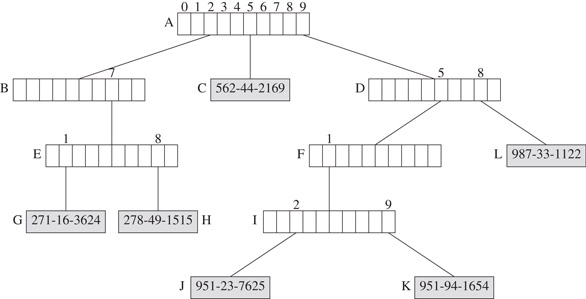
Figure 29.7Trie of Figure 29.1 with 987-33-1122 inserted.
To remove the element whose key is theKey, we first search for the element with this key. If there is no matching element in the trie, nothing is to be done. So, assume that the trie contains an element theElement whose key is theKey. The element node X that contains theElement is discarded, and we retrace the path from X to the root discarding branch nodes that are roots of subtries that have only 1 element in them. This path retracing stops when we either reach a branch node that is not discarded or we discard the root.
Consider the trie of Figure 29.7. When the element with key 951-23-7625 is removed, the element node J is discarded and we follow the path from node J to the root node A. The branch node I is discarded because the subtrie with root I contains the single element node K. We next reach the branch node F. This node is also discarded, and we proceed to the branch node D. Since the subtrie rooted at D has 2 element nodes (K and L), this branch node is not discarded. Instead, node K is made a child of this branch node, as is shown in Figure 29.8.

Figure 29.8Trie of Figure 29.7 with 951-23-7635 removed.
To remove the element with key 562-44-2169 from the trie of Figure 29.8, we discard the element node C. Since its parent node remains the root of a subtrie that has more than one element, the parent node is not discarded and the removal operation is complete. Figure 29.9 show the resulting trie.

Figure 29.9Trie of Figure 29.8 with 562-44-2169 removed.
The time required to remove an element with a d digit key from a radix r trie is O(dr) because the removal may require us to discard O(d) branch nodes and it takes O(r) time to determine whether a branch node is to be discarded. The complexity of the remove operation can be reduced to O(r + d) by adding a numberOfElementsInSubtrie field to each branch node.
29.8Prefix Search and Applications
You have probably realized that to search a trie we do not need the entire key. Most of the time, only the first few digits (i.e., a prefix) of the key is needed. For example, our search of the trie of Figure 29.1 for an element with key 951-23-7625 used only the first four digits of the key. The ability to search a trie using only the prefix of a key enables us to use tries in applications where only the prefix might be known or where we might desire the user to provide only a prefix. Some of these applications are described below.
Criminology
Suppose that you are at the scene of a crime and observe the first few characters CRX on the registration plate of the getaway car. If we have a trie of registration numbers, we can use the characters CRX to reach a subtrie that contains all registration numbers that begin with CRX. The elements in this subtrie can then be examined to see which cars satisfy other properties that might have been observed.
Automatic Command Completion
When using an operating system such as Unix or DOS, we type in system commands to accomplish certain tasks. For example, the Unix and DOS command cd may be used to change the current directory. Table 29.2 gives a list of commands that have the prefix ps (this list was obtained by executing the command ls/usr/local/bin/ps * on a Unix system).
Table 29.2Commands that Begin with “ps”
|
ps2ascii |
ps2pdf |
psbook |
psmandup |
psselect |
|
ps2epsi |
ps2pk |
pscal |
psmerge |
pstopnm |
|
ps2frag |
ps2ps |
psidtopgm |
psnup |
pstops |
|
ps2gif |
psbb |
pslatex |
psresize |
pstruct |
We can simply the task of typing in commands by providing a command completion facility which automatically types in the command suffix once the user has typed in a long enough prefix to uniquely identify the command. For instance, once the letters psi have been entered, we know that the command must be psidtopgm because there is only one command that has the prefix psi. In this case, we replace the need to type in a 9 character command name by the need to type in just the first 3 characters of the command!
A command completion system is easily implemented when the commands are stored in a trie using ASCII characters as the digits. As the user types the command digits from left to right, we move down the trie. The command may be completed as soon as we reach an element node. If we fall off the trie in the process, the user can be informed that no command with the typed prefix exists.
Although we have described command completion in the context of operating system commands, the facilty is useful in other environments:
1.A network browser keeps a history of the URLs of sites that you have visited. By organizing this history as a trie, the user need only type the prefix of a previously used URL and the browser can complete the URL.
2.A word processor can maintain a dictionary of words and can complete words as you type the text. Words can be completed as soon as you have typed a long enough prefix to identify the word uniquely.
3.An automatic phone dialer can maintain a list of frequently called telephone numbers as a trie. Once you have punched in a long enough prefix to uniquely identify the phone number, the dialer can complete the call for you.
Take a close look at the trie of Figure 29.1. This trie has a few branch nodes (nodes B, D, and F) that do not partition the elements in their subtrie into two or more nonempty groups. We often can improve both the time and space performance metrics of a trie by eliminating all branch nodes that have only one child. The resulting trie is called a compressed trie.
When branch nodes with a single child are removed from a trie, we need to keep additional information so that dictionary operations may be performed correctly. The additional information stored in three compressed trie structures is described below.
29.9.1Compressed Tries with Digit Numbers
In a compressed trie with digit numbers, each branch node has an additional field digitNumber that tells us which digit of the key is used to branch at this node. Figure 29.11 shows the compressed trie with digit numbers that corresponds to the trie of Figure 29.1. The leftmost field of each branch node of Figure 29.10 is the digitNumber field.
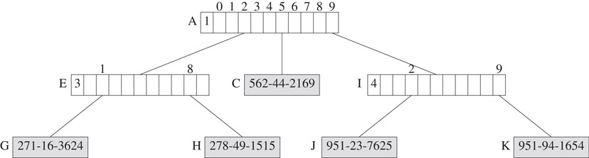
Figure 29.10Compressed trie with digit numbers.
29.9.1.1Searching a Compressed Trie with Digit Numbers
A compressed trie with digit numbers may be searched by following a path from the root. At each branch node, the digit, of the search key, given in the branch node’s digitNumber field is used to determine which subtrie to move to. For example, when searching the trie of Figure 29.10 for an element with key 951-23-7625, we start at the root of the trie. Since the root node is a branch node with digitNumber = 1, we use the first digit 9 of the search key to determine which subtrie to move to. A move to node A.child[9] = I is made. Since I.digitNumber = 4, the fourth digit, 2, of the search key tells us which subtrie to move to. A move is now made to node I.child[2] = J. We are now at an element node, and the search key is compared with the key of the element in node J. Since the keys match, we have found the desired element.
Notice that a search for an element with key 913-23-7625 also terminates at node J. However, the search key and the element key at node J do not match and we conclude that the trie contains no element with key 913-23-7625.
29.9.1.2Inserting into a Compressed Trie with Digit Numbers
To insert an element with key 987-26-1615 into the trie of Figure 29.10, we first search for an element with this key. The search ends at node J. Since the search key and the key, 951-23-7625, of the element in this node do not match, we conclude that the trie has no element whose key matches the search key. To insert the new element, we find the first digit where the search key differs from the key in node J and create a branch node for this digit. Since the first digit where the search key 987-26-1615 and the element key 951-23-7625 differ is the second digit, we create a branch node with digitNumber = 2. Since digit values increase as we go down the trie, the proper place to insert the new branch node can be determined by retracing the path from the root to node J and stopping as soon as either a node with digit value greater than 2 or the node J is reached. In the trie of Figure 29.10, this path retracing stops at node I. The new branch node is made the parent of node I, and we get the trie of Figure 29.11.

Figure 29.11Compressed trie following the insertion of 987-26-1615 into the compressed trie of Figure 29.10.
Consider inserting an element with key 958-36-4194 into the compressed trie of Figure 29.10. The search for an element with this key terminates when we fall of the trie by following the pointer I.child[3] = null. To complete the insertion, we must first find an element in the subtrie rooted at node I. This element is found by following a downward path from node I using (say) the first non null link in each branch node encountered. Doing this on the compressed trie of Figure 29.10, leads us to node J. Having reached an element node, we find the first digit where the element key and the search key differ and complete the insertion as in the previous example. Figure 29.12 shows the resulting compressed trie.

Figure 29.12Compressed trie following the insertion of 958-36-4194 into the compressed trie of Figure 29.10.
Because of the possible need to search for the first non null child pointer in each branch node, the time required to insert an element into a compressed tries with digit numbers is O(rd), where r is the trie radix and d is the maximum number of digits in any key.
29.9.1.3Removing an Element from a Compressed Trie with Digit Numbers
To remove an element whose key is theKey, we do the following:
1.Find the element node X that contains the element whose key is theKey.
2.Discard node X.
3.If the parent of X is left with only one child, discard the parent node also. When the parent of X is discarded, the sole remaining child of the parent of X becomes a child of the grandparent (if any) of X.
To remove the element with key 951-94-1654 from the compressed trie of Figure 29.12, we first locate the node K that contains the element that is to be removed. When this node is discarded, the parent I of K is left with only one child. Consequently, node I is also discarded, and the only remaining child J of node I is the made a child of the grandparent of K. Figure 29.13 shows the resulting compressed trie.
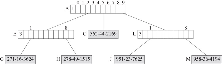
Figure 29.13Compressed trie following the removal of 951-94-1654 from the compressed trie of Figure 29.12.
Because of the need to determine whether a branch node is left with two or more children, removing a d digit element from a radix r trie takes O(d + r) time.
29.9.2Compressed Tries with Skip Fields
In a compressed trie with skip fields, each branch node has an additional field skip which tells us the number of branch nodes that were originally between the current branch node and its parent. Figure 29.15 shows the compressed trie with skip fields that corresponds to the trie of Figure 29.1. The leftmost field of each branch node of Figure 29.14 is the skip field.

Figure 29.14Compressed trie with skip fields.
The algorithms to search, insert, and remove are very similar to those used for a compressed trie with digit numbers.
29.9.3Compressed Tries with Edge Information
In a compressed trie with edge information, each branch node has the following additional information associated with it: a pointer/reference element to an element (or element node) in the subtrie, and an integer skip which equals the number of branch nodes eliminated between this branch node and its parent. Figure 29.15 shows the compressed trie with edge information that corresponds to the trie of Figure 29.1. The first field of each branch node is its element field, and the second field is the skip field.

Figure 29.15Compressed trie with edge information.
Even though we store the “edge information” with branch nodes, it is convenient to think of this information as being associated with the edge that comes into the branch node from its parent (when the branch node is not the root). When moving down a trie, we follow edges, and when an edge is followed. we skip over the number of digits given by the skip field of the edge information. The value of the digits that are skipped over may be determined by using the element field.
When moving from node A to node I of the compressed trie of Figure 29.15, we use digit 1 of the key to determine which child field of A is to be used. Also, we skip over the next 2 digits, that is, digits 2 and 3, of the keys of the elements in the subtrie rooted at I. Since all elements in the subtrie I have the same value for the digits that are skipped over, we can determine the value of these skipped over digits from any of the elements in the subtrie. Using the element field of the edge information, we access the element node J, and determine that the digits that are skipped over are 5 and 1.
29.9.3.1Searching a Compressed Trie with Edge Information
When searching a compressed trie with edge information, we can use the edge information to terminate unsuccessful searches (possibly) before we reach an element node or fall off the trie. As in the other compressed trie variants, the search is done by following a path from the root. Suppose we are searching the compressed trie of Figure 29.15 for an element with key 921-23-1234. Since the skip value for the root node is 0, we use the first digit 9 of the search key to determine which subtrie to move to. A move to node A.child[9] = I is made. By examining the edge information (stored in node I), we determine that, in making the move from node A to node I, the digits 5 and 1 are skipped. Since these digits do not agree with the next two digits of the search key, the search terminates with the conclusion that the trie contains no element whose key equals the search key.
29.9.3.2Inserting into a Compressed Trie with Edge Information
To insert an element with key 987-26-1615 into the compressed trie of Figure 29.15, we first search for an element with this key. The search terminates unsuccessfully when we move from node A to node I because of a mismatch between the skipped over digits and the corresponding digits of the search key. The first mismatch is at the first skipped over digit. Therefore, we insert a branch node L between nodes A and I. The skip value for this branch node is 0, and its element field is set to reference the element node for the newly inserted element. We must also change the skip value of I to 1. Figure 29.16 shows the resulting compressed trie.

Figure 29.16Compressed trie following the insertion of 987-26-1615 into the compressed trie of Figure 29.15.
Suppose we are to insert an element with key 958-36-4194 into the compressed trie of Figure 16. The search for an element with this key terminates when we move to node I because of a mismatch between the digits that are skipped over and the corresponding digits of the search key. A new branch node is inserted between nodes A and I and we get the compressed trie that is shown in Figure 29.17.

Figure 29.17Compressed trie following the insertion of 958-36-4194 into the compressed trie of Figure 29.15.
The time required to insert a d digit element into a radix r compressed trie with edge information is O(r + d).
29.9.3.3Removing an Element from a Compressed Trie with Edge Information
This is similar to removal from a compressed trie with digit numbers except for the need to update the element fields of branch nodes whose element field references the removed element.
29.9.4Space Required by a Compressed Trie
Since each branch node partitions the elements in its subtrie into two or more nonempty groups, an n element compressed trie has at most n − 1 branch nodes. Therefore, the space required by each of the compressed trie variants described by us is O(nr), where r is the trie radix.
When compressed tries are represented as hash tables, we need an additional data structure to store the nonpointer fields of branch nodes. We may use an array (much like we use the array information) for this purpose.
The data structure Patricia (Practical Algorithm To Retrieve Information Coded In Alphanumeric) is a compressed binary trie in which the branch and element nodes have been melded into a single node type. Consider the compressed binary trie of Figure 29.18. Circular nodes are branch nodes and rectangular nodes are element nodes. The number inside a branch node is its bit number field; the left child of a branch node corresponds to the case when the appropriate key bit is 0 and the right child to the case when this bit is 1. The melding of branch and element nodes is done by moving each element from its element node to an ancestor branch node. Since the number of branch nodes is one less than the number of element nodes, we introduce a header node and make the compressed binary trie the left subtree of the header. Pointers that originally went from a branch node to an element node now go from that branch node to the branch node into which the corresponding element has been melded. Figure 29.19 shows a possible result of melding the nodes of Figure 29.18. The number outside a node is its bit number values. The thick pointers are backward pointers that replace branch-node to element-node pointers in Figure 29.18. A backward pointer has the property that the bit number value at the start of the pointer is ≥ the bit number value at its end. For original branch-node to branch-node pointers (also called downward pointers), the bit number value at the pointer end is always greater than the bit number value at the pointer start.
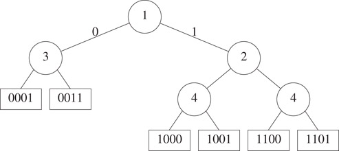
Figure 29.18A compressed binary trie.

Figure 29.19A Patricia instance that corresponds to Figure 29.18.
To search for an element with key theKey, we use the bits of theKey from left to right to move down the Patricia instance just as we would search a compressed binary trie. When a backward pointer is followed, we compare theKey with the key in the reached Patricia node. For example, to search for theKey = 1101, we start by moving into the left subtree of the header node. The pointer that is followed is a downward pointer (start bit number is 0 and end bit number is 1). We branch using bit 1 of theKey. Since this bit is 1, we follow the right child pointer. The start bit number for this pointer is 1 and the end bit number is 2. So, again, a downward pointer has been followed. The bit number for the reached node is 2. So, we use bit 2 of theKey to move further. Bit 2 is a 1. So, we use the right child pointer to get to the node that contains 1100. Again, a downward pointer was used. From this node, a move is made using bit 4 of theKey. This gets us to the node that contains 1101. This time, a backward pointer was followed (start bit of pointer is 4 and end bit is 1). When a backward pointer is followed, we compare theKey with the key in the reached node. In this case, the keys match and we have found the desired element. Notice that the same search path is taken when theKey = 1111. In this case, the final compare fails and we conclude that we have no element whose key is 1111.
We use an example to illustrate the insert algorithm. We start with an empty instance. Such an instance has no node; not even the header. For our example, we will consider keys that have 7 bits. For the first insert, we use the key 0000101. When inserting into an empty instance, we create a header node whose left child pointer points to the header node; the new element is inserted into the header; and the bit number field of the header set to 0. The configuration of Figure 29.20a results. Note that the right child field of the header node is not used.

Figure 29.20Insertion example.
The key for the next insert is 0000000. The search for this key terminates at the header. We compare the insert key and the header key and determine that the first bit at which they differ is bit 5. So, we create a new node with bit number field 5 and insert the new element into this node. Since bit 5 of the insert key is 0, the left child pointer of the new node points to the new node and the right child pointer to the header node (Figure 29.20b).
For the next insertion, assume that the key is 0000010. The search for this key terminates at the node with 0000000. Comparing the two keys, we determine that the first bit at which the two keys differ is bit 6. So, we create a new node with bit number field 6 and put the new element into this new node. The new node is inserted into the search path in such a way that bit number fields increase along this path. For our example, the new node is inserted as the left child of the node with 0000000. Since bit 6 of the insert key is 1, the right child pointer of the new node is a self pointer and the left child pointer points to the node with 0000000. Figure 29.20c shows the result.
The general strategy to insert an element other than the first one is given below. The key of the element to be inserted is theKey.
1.Search for theKey. Let reachedKey be the key in the node endNode where the search terminates.
2.Determine the leftmost bit position lBitPos at which theKey and reachedKey differ. lBitPos is well defined so long as one of the two keys isn’t a prefix of the other.
3.Create a new node with bit number field lBitPos. Insert this node into the search path from the header to endNode so that bit numbers increase along this path. This insertion breaks a pointer from node p to node q. The pointer now goes from p to the new node.
4.If bit lBitPos of theKey is 1, the right child pointer of the new node becomes a self pointer (i.e., it points to the new node); otherwise, the left child pointer of the new node becomes a self pointer. The remaining child pointer of the new node points to q.
For our next insert, the insert key is 0001000. The search for this key terminates at the node with 0000000. We determine that the first bit at which the insert key and reachedKey = 0000000 differ is bit 4. We create a new node with bit number 4 and put the new element into this node. The new node is inserted on the search path so as to ensure that bit number fields increase along this path. So, the new node is inserted as the left child of the header node (Figure 29.18d). This breaks the pointer from the header to the node q with 0000000. Since bit 4 of the insert key is 1, the right child pointer of the new node is a self pointer and the left child pointer goes to node q.
We consider two more inserts. Consider inserting an element whose key is 0000100. The reached key is 0000101 (in the header). We see that the first bit at which the insert and reached keys differ is bit 7. So, we create a new node with bit number 7; the new element is put into the new node; the new node is inserted into the search path so as to ensure that bit numbers increase along this path (this requires the new node to be made a right child of the node with 0000000, breaking the child pointer from 0000000 to the header); for the broken pointer, p is the node with 0000000 and q is the header; the left child pointer of the new node is a self pointer (because bit 7 of the insert key is 0); and remaining child pointer (in this case the right child) of the new node points to q (see Figure 29.21a).

Figure 29.21Insertion example.
For our final insert, the insert key is 0001010. A search for this key terminates at the node with 0000100. The first bit at which the insert and reached keys differ is bit 6. So, we create a new node with bit number 6; the new element is put into the new node; the new node is inserted into the search path so as to ensure that bit numbers increase along this path (this requires the new node to be made a right child of the node with 0001000; so, p = q = node with 001000); the right child pointer of the new node is a self pointer (because bit 6 of the insert key is 1); and the remaining child (in this case the left child) of the new node is q (see Figure 29.21b).
Let p be the node that contains the element that is to be removed. We consider two cases for p—(a) p has a self pointer and (b) p has no self pointer. When p has a self pointer and p is the header, the Patricia instance becomes empty following the element removal (Figure 29.20a). In this case, we simply dispose of the header. When p has a self pointer and p is not the header, we set the pointer from the parent of p to the value of p’s non-self pointer. Following this pointer change, the node p is disposed. For example, to remove the element with key 0000010 from Figure 29.21a, we change the left child pointer in the node with 0000000 to point to the node pointed at by p’s non-self pointer (i.e., the node with 0000000). This causes the left child pointer of 0000000 to become a self pointer. The node with 0000010 is then disposed.
For the second case, we first find the node q that has a backward pointer to node p. For example, when we are to remove 0001000 from Figure 29.21b, the node q is the node with 0001010. The element qElement in q (in our example, 0001010) is moved to node p and we proceed to delete node q instead of node p. Notice that node q is the node from which we reached node p in the search for the element that is to be removed. To delete node q, we first find the node r that has a back pointer to q (for our example r = q). The node r is found by using the key of qElement. Once r is found, the back pointer to q that is in r is changed from q to p to properly account for the fact that we have moved qElement to p. Finally, the downward pointer from the parent of q to q is changed to q’s child pointer that was used to locate r. In our example p is the parent of q and the right child pointer of p is changed from q to the right child of q, which itself was just changed to p.
We see that the time for each of the Patricia operations search, insert, and delete is O(h), where h is the height of the Patricia instance. For more information on Patricia and general tries, see [2,3].
This work was supported, in part, by the National Science Foundation under grant CCR-9912395.
1.A. Andersson and S. Nillson, Improved behavior of tries by adaptive branching, Information Processing Letters, 46, 1993, 295–300.
2.E. Horowitz, S. Sahni, and D. Mehta, Fundamentals of Data Structures in C++, Computer Science Press, 1995.
3.D. Knuth, The Art of Computer Programming: Sorting and Searching, Second Edition, Addison-Wesley, 1998.
*This chapter has been reprinted from first edition of this Handbook, without any content updates.
*The definition of height used in this chapter is: the height of a trie equals the number of levels in that trie.