
Andrzej Ehrenfeucht
University of Colorado
Ross M. McConnell
Colorado State University
A Simple Algorithm for Constructing the DAWG•Constructing the DAWG in Linear Time
Using the Compact DAWG to Find the Locations of a String in the Text•Variations and Applications
Building the Position Heap•Querying the Position Heap•Time Bounds•Improvements to the Time Bounds
Searching for occurrences of a substring in a text is a common operation familiar to anyone who uses a text editor, word processor, or web browser. It is also the case that algorithms for analyzing textual databases can generate a large number of searches. If a text, such as a portion of the genome of an organism, is to be searched repeatedly, it is sometimes the case that it pays to preprocess the text to create a data structure that facilitates the searches. The suffix tree [1] and suffix array [2] discussed in Chapter 30 are examples.
In this chapter, we give some alternatives to these data structures that have advantages over them in some circumstances, depending on what type of searches or analysis of the text are desired, the amount of memory available, and the amount of effort to be invested in an implementation.
In particular, we focus on the problem of finding the locations of all occurrences of a string x in a text t, where the letters of t are drawn from a fixed alphabet Σ, such as the ASCII letter codes.
The length of a string x, denoted |x|, is the number of characters in it. The empty string, denoted λ is the string of length 0 that has no characters in it. If t = a1a2, …, an is a text and is a substring of it, then i is a starting position of p in t and j is an ending position of p in t. For instance, the starting positions of abc in aabcabcaac are {2, 5}, and its ending positions are {5, 8}. We consider the empty string to have starting and ending positions at {0, 1, 2, …, n}, once at each position in the text, and once at position 0, preceding the first character of the text. Let EndPositions(p, t) denote the ending positions of p in t; when t is understood, we may denote it EndPositions(p).
A deterministic finite automaton on Σ is a directed graph where each directed edge is labeled with a letter from Σ, and where, for each node, there is at most one edge directed out of the node that is labeled with any given letter. Exactly one of the nodes is designated as a start node, and some of the nodes are designated as accept nodes. The label of a directed path is the word given by the sequence of letters on the path. A deterministic finite automaton is used for representing a set of words, namely, the set of labels of paths from the start node to an accept node.
The first data structure that we examine is the directed acyclic word graph (DAWG). The DAWG is just a deterministic finite automaton representing the language of subwords of a text t, which is finite, hence regular. All of its states except for one are accept states. There is no edge from the nonaccepting state to any accepting state, so it is convenient to omit the nonaccept state when representing the DAWG. In this representation, a string p is a substring of t iff it is the label of a directed path originating at the start node.
There exists a labeling of each node of the DAWG with a set of positions so that the DAWG has the following property:
•Whenever p is a substring of t, its ending positions in t are given by the label of the last node of the path of label p that originates at the start node.
To find the locations where p occurs, one need only begin at the start node, follow edges that match the letters of p in order, and retrieve the set of positions at the node where this process halts.
In view of the fact that there are Θ(|t|2) intervals on t, each of which represents a substring that is contained in the interval, it is surprising that the number of nodes and edges of the DAWG of t is O(|t|). The reason for this is that all possible query strings fall naturally into equivalence classes, which are sets of strings such that two strings are in the same set if they have the same set of ending positions. The size of an equivalence class can be large, and this economy makes the O(|t|) bound possible.
In an application such as a search engine, one may be interested not in the locations of a string in a text, but the number of occurrences of a string in the text. This is one criterion for deciding which texts are most relevant to a query. Since all strings in an equivalence class have the same number of occurrences, each state can be labeled not with the position set, but with the cardinality of its position set. The label of the node reached on the path labeled p originating at the start node tells the number of occurrences of p in t in O(|p|) time. This variant requires O(|t|) space and can be constructed in O(|t|) time.
Unfortunately, the sum of cardinalities of the position sets of the nodes of the DAWG of t is not O(|t|). However, a second data structure that we describe, called the compact DAWG does use O(|t|) space. If a string p has k occurrences in t, then it takes O(|p| + k) time to return the set of occurrences where p occurs in t, given the compact DAWG of t. It can be built in O(|t|) time. These bounds are the same as that for the suffix tree and suffix array, but the compact DAWG requires substantially less space in most cases. An example is illustrated in Figure 31.2.
Another important issue is the ease with which a programmer can understand and program the construction algorithm. Like the computer time required for queries, the time spent by a programmer understanding, writing, and maintaining a program is also a resource that must be considered. The third data structure that we present, called the position heap, has worse worst-case bounds for construction and queries, but has the advantage of being as easy to understand and construct as elementary data structures such as unbalanced binary search trees and heaps. One trade-off is that the worst-case bounds for a query is O(|p|2 + k), rather than O(|p| + k). However, on randomly generated strings, the expected time for a query is O(|p| + k), and on most practical applications, the query time can be expected not to differ greatly from this. Like the other structures, it can be constructed in linear time. However, an extremely simple implementation takes O(|t| log |t|) expected time on randomly generated strings and does not depart much from this in most practical applications. Those who wish to expend minimal programming effort may wish to consider this simple variant of the construction algorithm.
The position heap for the string of Figure 31.1 is illustrated in Figure 31.3.

Figure 31.1The DAWG of the text aabcabcaac. The starting node is at the upper left. A string p is a substring of the text if and only if it is the label of a path originating at the start node. The nodes can be labeled so that whenever p is the label of such a path, the last node of the path gives EndPositions(p). For instance, the strings that lead to the state labeled {5, 8} are ca, bca, and abca, and these have occurrences in the text with their last letter at positions 5 and 8.

Figure 31.2The compact DAWG of the text aabcabcaac (cf. Figure 31.1) The labels depicted in the nodes are the ending positions of the corresponding principal nodes of the DAWG. The compact DAWG is obtained from the DAWG by deleting nodes that have only one outgoing edge, and representing deleted paths between the remaining nodes with edges that are labeled with the path’s label.
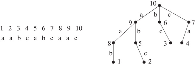
Figure 31.3The position heap of aabcabcaa.
More recently, an alternative to the construction algorithm given here has been given in Reference 3. That algorithm can be considered online, since it can construct the position heap incrementally as characters are appended to the text. The algorithm we give here can construct it as characters are prepended to the text. The case where they are appended can be reduced to the case where they are prepended, by working with the reverse of the text and reversing query strings before each query. The algorithm of Reference 3 is more natural for this and contributes additional algorithmic insights.
This analysis assumes that the size of the alphabet is a constant, which is a reasonable assumption for genomic sequences, for example. Recently, an algorithm that takes linear time, independently of the size of the alphabet, has been given in Reference 4. However, a step of that algorithm is construction of the suffix tree, hence it is conceptually more difficult than the one given here.
Linear-time construction of the position heap for a set of strings stored as a trie is given in Reference 5.
The infinite set of all strings that can be formed from letters of an alphabet Σ is denoted as Σ*. If a ∈ Σ, let an denote the string that consists of n repetitions of a.
If x is a string, then for 1 ≤ j ≤ |x|, let xj denote the character in position j. Thus x can be written as x1x2, …, x|x|. The reversal xR of x is the string . Let x[i : j] denote the substring .
The prefixes of a string x = x1x2, …, xk are those with a starting position at the leftmost position of x, namely, the empty string and those strings of the form x[1 : j] for 1 ≤ j ≤ k. Its suffixes are those with an ending position at the rightmost position of x, namely, the empty string and those of the form x[j : k].
A trie on Σ is a deterministic finite automaton that is a rooted tree whose start node is the root.
Given a family of subsets of a domain , the transitive reduction of the subset relation can be viewed as a pointer from each to each such that X ⊂ Y and there exists no Z such that X ⊂ Z ⊂ Y. This is sometimes referred to as the Hasse diagram of the subset relation on the family. The Hasse diagram is a tree if , , and for each , either X ⊆ Y, Y ⊂ X, or X ∩ Y = ∅.
Lemma 31.1
Let x and y be two strings such that EndPositions(x) ∩ EndPositions(y) ≠ ∅. One of x and y must be a suffix of the other, and either EndPositions(x) = EndPositions(y), EndPositions(x) ⊂ EndPositions(y), or EndPositions(y) ⊂ EndPositions(x).
Proof. If x and y have a common ending position i, then the two occurrences coincide in a way that forces one to be a suffix of the other. Suppose without loss of generality that y is a suffix of x. Then every occurrence of x contains an occurrence of y inside of it that ends at the same position, so Endpositions(x) ⊆ Endpositions(y).■
For instance, in the string aabcabcaac, the string ca has ending positions {5, 8}, while the string aabca has ending positions {5}, and ca is a suffix of aabca.
Let x’s right-equivalence class in t be the set {y|EndPositions(y) = EndPositions(x)}. The only infinite class is degenerate class of strings with the empty set as ending positions, namely, those elements of Σ* that are not substrings of t.
The right-equivalence classes on t are a partition of Σ*: each member of Σ* is in one and only one right-equivalence class. By Lemma 31.1, whenever two strings are in the same nondegenerate right-equivalence class, then one of them is a suffix of the other. It is easily seen that if y is the shortest string in the class and x is the longest, then the class consists of the suffixes of x whose length is at least |y|. For instance, in Figure 31.1, the class of strings with end positions {5, 8} consists of y = ca, x = abca, and since bca is a longer suffix of x than y is.
Lemma 31.2
A text t of length n has at most 2n right-equivalence classes.
Proof. The degenerate class is one right equivalence class. All others have nonempty ending positions, and we must show that there are at most 2n − 1 of them. The set V = {0, 1, 2, …, n} is the set of ending positions of the empty string. If X and Y are sets of ending positions of two right-equivalence classes, then X ⊆ Y, Y ⊆ X, or Y ∩ X = ∅, by Lemma 31.1. Therefore, the transitive reduction (Hasse diagram) of the subset relation on the nonempty position sets is a tree rooted at V. For any i such that {i} is not a leaf, we can add {i} as a child of the lowest set that contains i as a member. The leaves are now a partition of {1, 2, …, n} so it has at most n leaves. Since each node of the tree has at least two children, there are at most 2n − 1 nodes.■
Definition 31.1
The DAWG is defined as follows. The states of the DAWG are the nondegenerate right-equivalence classes that t induces on its substrings. For each a ∈ Σ and x ∈ Σ* such that xa is a substring of t, there is an edge labeled a from x’s right-equivalence class to xa’s right-equivalence class.
Figure 31.1 depicts the DAWG by labeling each right-equivalence class with its set of ending positions. The set of words in a class is just the set of path labels of paths leading from the source to a class. For instance, the right-equivalence class represented by the node labeled {5, 8} is {ca, bca, abca}.
It would be natural to include the infinite degenerate class of strings that do not occur in t. This would ensure that every state had an outgoing edge for every letter of Σ. However, it is convenient to omit this state when representing the DAWG: for each a ∈ Σ, there is an edge from the degenerate class to itself, and this does not need to be represented explicitly. An edge labeled a from a nondegenerate class to the degenerate class is implied by the absence of an edge out of the state labeled a in the representation.
For each node X and each a ∈ Σ, there is at most one transition out of X that is labeled a. Therefore, the DAWG is a deterministic finite automaton. Any word p such that EndPositions(p) ≠ ∅ spells out the labels of a path to the state corresponding to EndPositions(p). Therefore, all states of the DAWG are reachable from the start state. The DAWG cannot have a directed cycle, as this would allow an infinite set of words to spell out a path, and the set of subwords of t is finite. Therefore, it can be represented by a directed acyclic graph.
A state is a sink if it has no outgoing edges. A sink must be the right-equivalence class containing position n, so there is exactly one sink.
Theorem 31.1
The DAWG for a text of length n has at most 2n − 1 nodes and 3n − 3 edges.
Proof. The number of nodes follows from Lemma 31.2. There is a single sink, namely, the one that has position set {|t|}, this represents the equivalence class containing those suffixes of t that have a unique occurrence in t. Let T be a directed spanning tree of the DAWG rooted at the start state. T has one fewer edges than the number of states, hence 2n − 2 edges. For every e ∉ T, let P1(e) denote the path in T from the start state to the tail of e, let P2(e) denote an arbitrary path in the DAWG from the head of e to the sink, and let P(e) denote the concatenation of (P1(e), e, P2(e)). Since P(e) ends at the sink, the labels of its edges yield a suffix of t. For e1, e2 ∉ T with e1 ≠ e2, P(e1) ≠ P(e2), since they differ in their first edge that is not in T. One suffix is given by the labels of the path in T to the sink. Each of the remaining n − 1 suffixes is the sequence of labels of P(e) for at most one edge e ∉ T, so there are at most n − 1 edges not in T.
The total number of edges of the DAWG is bounded by 2n − 2 tree edges and n − 1 nontree edges.■
To determine whether a string p occurs as a substring of t, one may begin at the start state and either find the path that spells out the letters of p, thereby accepting p, or else reject p if there is no such path. This requires finding, at each node x, the transition labeled a leaving x, where a is the next letter of p. If |Σ| = O(1), this takes O(1) time, so it takes O(|p|) time to determine whether p is a subword of t. Note that, in contrast to naive approaches to this problem, this time bound is independent of the length of t.
If the nodes of the DAWG are explicitly labeled with the corresponding end positions, as in Figure 31.1, then it is easy to find the positions where a substring occurs: it is the label of the state reached on the substring. However, doing this is infeasible if one wishes to build the DAWG in O(|t|) time and use O(|t|) storage, since the sum of cardinalities of the position sets can be greater than this. For this problem, it is preferable to use the compact DAWG that is described below.
For the problem of finding the number of occurrences of a substring in t, it suffices to label each node with the number of positions in its position set. This may be done in postorder in a depth-first search, starting at the start node, and applying the following rule: the label of a node v is the sum of labels of its outneighbors, which have already been labeled by the time one must label v. Handling v takes time proportional to the number of edges originating at v, which we have already shown is O(|t|).
31.3.1A Simple Algorithm for Constructing the DAWG
Definition 31.2
If x is a substring of t, let us say that x’s redundancy in t is the number of ending (or beginning) positions it has in t. If i is a position in t, let h(i) be the longest substring x of t with an ending position at i whose redundancy is at least as great as its length, |x|. Let h(t) be the average of h(i) over all i, namely .
Clearly, h(t) is a measure of how redundant t is; the greater the value of h(t), the less information it can contain.
In this section, we given an O(|t|h(t)) algorithm for constructing the DAWG of a string t. This is quadratic in the worst case, which is illustrated by the string t = an, consisting of n copies of one letter. However, we claim that the algorithm is a practical one for most applications, where h(t) is rarely large even when t has a long repeated substring. In most applications, h(t) can be expected to behave like an O(log|t|) function.
The algorithm explicitly labels the nodes of the DAWG with their ending positions, as illustrated in Figure 31.1. Each set of ending positions is represented with a list, where the positions appear in ascending order. It begins by creating a start node, and then iteratively processes an unprocessed node by creating its neighbors. To identify an unprocessed node, it is convenient to keep a list of the unprocessed nodes, insert a node in this list, and remove a node from the front of the list when it is time to process a new node.
Algorithm 31.1
DAWGBuild(t)
    Create a start node with position set {0,1,…,n}
    While there is an unprocessed node v
       Create a copy of v’s position set
       Add 1 to every element of this set
       Remove n + 1 from this copy if it occurs
       Partition the copy into sets of positions that have a common letter
       For each partition class W
           If W is already the position set of a node, then let w denote that node
           Else create a new node w with position set W
           Let a be the letter that occurs at the positions in W
           Install an edge labeled a from v to w
Figure 31.4 gives an illustration. For the correctness, it is easy to see by induction on k that every substring w of the text that has length k leads to a node whose position set is the ending positions of w.
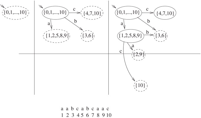
Figure 31.4Illustration of the first three iterations of Algorithm31.1 on aabcabcaac. Unprocessed nodes are drawn with dashed outlines. The algorithm initially creates a start state with position set {0, 1, …, n} (left figure). To process the start node, it creates a copy of this position set and adds 1 to each element, yielding {1, 2, …, n + 1}. It discards n + 1, yielding {1, 2, …, n}. It partitions this into the set {1, 2, 5, 8, 9} of positions that contain a, the set {3, 6} of positions that contain b, and the set {4, 7, 10} of positions that contain c, creates a node for each, and installs edges labeled with the corresponding letters to the new nodes (middle figure). To process the node v labeled {1, 2, 5, 8, 9}, it adds 1 to each element of this set to obtain {2, 3, 6, 9, 10}, and partitions them into {2, 9}, {3, 6}, and {10}. Of these, {2, 9} and {10} are new position sets, so a new node is created for each. It then installs edges from v to the nodes with these three position sets.
Lemma 31.3
The sum of cardinalities of the position sets of the nodes of the DAWG is O(|t|h(t)).
Proof. For a position i, let N(i) be the number of ending position sets in which position i appears. By Lemma 31.1, position sets that contain i form a chain {X1, X2, …, XN(i)}, where for each i from 1 to N(i) − 1, |Xi| > |Xi + 1|, and a string with Xi as its ending positions must be shorter than one with Xi + 1 as its ending positions. Therefore, |X⌊N(i)/2⌋| ≥ N(i)/2, and any string with this set as its ending position set must have length at least ⌊(N(i)/2⌋ − 1. This is a string whose set of ending positions is at least as large as its length, so N(i) = O(h(t)).
The sum of cardinalities of the position sets is given by , since each appearance of i in a position set contributes 1 to the sum, and this sum is O(|t|h(T)).■
It is easy to keep the classes as sorted linked lists. When a class X is partitioned into smaller classes, these fall naturally into smaller sorted lists in time linear in the size of X. A variety of data structures, such as tries, are suitable for looking up whether the sorted representation of a class W already occurs as the position set of a node. The time is therefore linear in the sum of cardinalities of the position sets, which is O(|t|h(t)) by Lemma 31.3.
31.3.2Constructing the DAWG in Linear Time
The linear-time algorithm given in Reference 6 to construct the DAWG works incrementally by induction on the length of the string. The DAWG of a string of length 0 (the null string) is just a single start node. For k = 0 to n − 1, it iteratively performs an induction step that modifies the DAWG of t[1 : k] to obtain the DAWG of t[1 : k +c1].
To gain insight into how the induction step must be performed, consider Figure 31.5. An occurrence of a substring of t can be specified by giving its ending position and its length. For each occurrence of a substring, it gives the number of times the substring occurs up to that point in the text, indexed by length and position. For instance, the string that has length 3 and ends at position 5 is bca. The entry in row 3, column 5 indicates that there is one occurrence of it up through position 5 of the text. There is another at position 8, and the entry at row 3 column 8 indicates that it has two occurrences up through position 8.
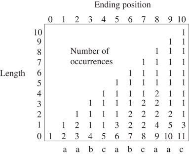
Figure 31.5Displaying the number of occurrences of substrings in a text. In the upper figure, the entry in row i column j corresponds to the substring of length j that ends at position i in the text t, and gives the number of occurrences of the substring at position i or before. That is, it gives the number of occurrences of the substring in t[1 : i]. Row 0 is included to reflect occurrences of the null substring, which has occurrences at {0, 1, …, n}.
The lower figure, which we may call the incremental landscape, gives a simplified representation of the table, by giving an entry only if it differs from the entry immediately above it. Let L[i, j] denote the entry in row i, column k of the incremental landscape. Some of these entries are blank; the implicit value of such an entry is the value of the first nonblank entry above it.
Column k has one entry for each right-equivalence class of t[1 : k] that has k as an ending position. For instance, in column 8, we see the following:
1.L[0, 8]: A right-equivalence class for the suffix of t[1 : 8] of length 0, namely, the empty string, which has nine occurrences ({0, 1, …, 8}) in t[1 : 8].
2.L[1, 8]: A right-equivalence class for the suffix of t[1 : 8] of length 1, namely, the suffix a, which has four occurrences ({1, 2, 5, 8}) in t[1 : 8].
3.L[4, 8]: A right-equivalence class for suffixes of t[1 : 8] of lengths 2 through 4, namely, {ca, bca, abca}, which have two occurrences ({5, 8}) in t[1 : 8]. The longest of these, abca, is given by the nonblank entry at L[4, 8], and membership of the others in the class is given implicitly by the blank entries immediately below it.
4.L[8, 8]: A right-equivalence class for suffixes of t[1 : k] of lengths 5 through 8, namely, {cabca, bcabca, abcabca, abcabca} that have one occurrence in t[1 : 8].
We may therefore treat nonblank entries in the incremental landscape as nodes of the DAWG. Let the height of a node denote the length of the longest substring in its right-equivalence class; this is the height (row number) where it appears in the incremental landscape.
When modifying the DAWG of t[1 : k] to obtain the DAWG of t[1 : k + 1], all new nodes that must be added to the DAWG appear in column k + 1. However, not every node in column k + 1 is a new node, as some of the entries reflect nodes that were created earlier.
For instance, consider Figure 31.7, which shows the incremental step from t[1 : 6] to t[1 : 7]. One of the nodes, which represents the class {cabc, bcabc, abcabc, aabcabc} of substrings of t[1 : 7] that are not substrings of t[1 : 6]. It is the top circled node of column 7 in Figure 31.6. Another represents the class Z2 = {c, bc, abc}. This appears in L[3, 7]. To see why this is new, look at the previous occurrence of its longest substring, abc, which is represented by L[3, 4], which is blank. Therefore, in the DAWG of t[1 : 6], it is part of a right-equivalence Z, which appears at L[4, 4], and which contains a longer word, aabc. Since {c, bc, abc} are suffixes of t[1 : 7] and aabc is not, they cease to be right-equivalent in t[1 : 7]. Therefore, Z must be split into two right-equivalence classes, Z2 = {c, bc, abc} and Z1 = Z − Z2 = {aabc}. Let us call this operation a split.

Figure 31.6The incremental landscape is a simplification of the table of Figure 31.5, where an entry is displayed only if it differs from the entry above it. The entries in column i are right-equivalence classes of t[1 : i]. These are right-equivalence classes that may be affected during the induction step, when the DAWG of t[1 : i − 1] is modified to obtain the DAWG of t[1 : i]. Equivalence classes of t[i : 1] that are not right-equivalence classes in t[1 : i] are circled; these correspond to nodes of the DAWG that must be created during the induction step. Edges of the DAWG of t[1 : i] from classes in column i − 1 are depicted as arrows. (The distinction between solid and dashed arrows is used in the proof of Theorem 31.2.)

Figure 31.7Modifying the DAWG of t[1 : 6] = aabcab to obtain the DAWG of t[1 : 7] = aabcabc. New nodes are shown with bold outlines. The sixth column of the incremental landscape, from top to bottom, consists of the nodes {6}, {3, 6}, and the start node. The seventh column, from top to bottom, consists of {7}, {4, 7}, and the start node. The node {4, 7} is split from {4}; of the strings {c, bc, abc, aabc} that end at node {4}, only {c, bc, abc} also occur at position 7, so these must now be handled by a different node from the one that handles aabc. All edges from nodes in the previous column to {4} are redirected to the new node {4, 7}.
Let us say that a node is new in column k if it is created when the DAWG of t[1 : k] is modified to obtain the DAWG of t[1 : k + 1]. In Figure 31.6, a node in a column is circled if it is new in that column. In general, a node is new in column k iff it is the top node of the column or the previous occurrence of its longest member corresponds to a blank space in the incremental landscape.
An important point is that only the top two nodes of a column can be new.
Lemma 31.4
If a new node is the result of a split, only one node lies above it in its column.
Proof. Let a be the character that causes the split, and let xa be the largest string in Z2, and let bxa be the smallest string in Z1 = Z − Z2. Since bxa previously had the same set of ending positions as xa and now it does not, it must be that xa occurs as a suffix of tk, but bxa does not. Let cxa be the smallest string in the next higher class C in column k + 1. On all previous occurrences of xa, it was inside bxa, so the first occurrence of cxa is at position k + 1. The frequency of the strings in C must be 1, so C is the top class of the column.■
The foregoing shows how nodes must be added to the DAWG in the inductive step. In order to understand how the edges of the DAWG must be modified, note that every edge directed into a node in column k + 1 comes from a node in column k. These edges are given by the following rule:
Lemma 31.5
In the DAWG of t[1 : k + 1], a node of height i in column k has an edge labeled tk + 1 to the lowest node of column k + 1 that has height greater than i.
These edges are drawn in as solid and dashed arrows in Figure 31.6. According to the figure, when the DAWG of t[1 : 7] is obtained from t[1 : 6], the new top node in the column must have an incoming edge from the top node of column 6, which is labeled {6} in Figure 31.7. The second new node in column 7, which is labeled {4, 7} in the figure, must have edges from the nodes at L[0, 6] and L[2, 6], which are the source and the node labeled {3, 6}. These are obtained by diverting edges into Z.
The induction step consists of implicitly marching in parallel down columns k and k + 1, creating the required nodes in column tk + 1 and installing the appropriate edges from right-equivalence classes in column k to right-equivalence classes of column k + 1, as well as the appropriate outgoing edges and parent pointers on each right-equivalence class in column k + 1 that is new in tk + 1. The new nodes in column k + 1 are the one with frequency one, and possibly one other, Z2, that results from a split. By Lemma 31.4, this requires marching down through at most two nodes of column k + 1, but possibly through many nodes of column k.
To facilitate marching down a column k efficiently, the algorithm needs a suffix pointer Suffix(x) on each node x of column k to the next lower node in column k. If y = y1y2y3…yj is the shortest string in the x’s right-equivalence class, then Suffix(x) points to the right-equivalence class that contains the longest proper suffix y2y3…yj of y. The suffix pointer for each node is uniquely defined, so the algorithm ensures that suffix pointers are available on nodes of column k by keeping suffix pointers current on all nodes of the DAWG.
The induction step is given in Algorithm 31.2. The algorithm does not build the incremental landscape. However, we may identify the nodes by where they would go in the incremental landscape. The meanings of the variables can be summarized as follows. Topk is the top node of column k, and Topk + 1 is the top node of column k + 1. Mid denotes the highest node of column k that already has an outgoing labeled with the (k + 1)th letter. The variable curNode is a looping variable that travels down through nodes of column k, becoming undefined if it travels past the bottom node of the column.
Algorithm 31.2
Update(Topk): Update the DAWG of t[1 : k] to obtain the DAWG of t[1 : k + 1]. Create a nodeTopk + 1 of frequency 1 and height k + 1 LetcurNode=Topk WhilecurNodeis defined and has no outgoing edge labeled tk + 1 Install an edge labeled tk + 1 fromcurNodetoTopk + 1curNode:=Suffix(curNode) IfcurNodeis definedMid:=curNodeLet Z be the neighbor ofMidon tk + 1 DefineSuffix(Topk + 1) to be Z Ifheight(Z) >height(Mid) + 1Split(k,Mid, Z); Create a second new node in Column k + 1 Else defineSuffix(Topk + 1) to be the start node Return Topk + 1 ProcedureSplit(k,Mid, Z) Create a copy Z2 of the node representing Z, together with its outgoing edges Let the height of Z2 be one plus the height ofMidLet curNode =MidWhilecurNodeis defined and Z is its neighbor on tk + 1 DivertcurNode’s edge labeled tk + 1 so that it points to Z2curNode:=Suffix(curNode) RedefineSuffix(Z2) to beSuffix(Z) RedefineSuffix(Z) to be Z2
Theorem 31.2
It takes O(|t|) time to build the DAWG of a text t of length n.
Proof. No node is ever discarded once it is created, and the final DAWG has O(|t|) nodes. Therefore, the cost of creating nodes is O(|t|). Once an edge is created it remains in the DAWG, though it might be diverted in calls to Split. No edge is ever discarded and the final DAWG has O(|t|) edges, so the cost of creating edges is O(|t|).
It remains to bound the cost of diverting edges in calls to Split. Let an edge that appears in the incremental landscape be solid if it goes from a node of height i to one of height i + 1, and dashed otherwise (see Figure 31.6). We may partition the edges in the landscape into terminating paths, each of which starts in row 0, and contains zero or more solid edges, and either followed by a dashed edge or ending in the last column. At most one terminating path begins in any column, and every dashed edge terminates a path. Thus there are at most n dashed edges.
When Z2 is created in Split, at most one of the edges diverted into it is solid. The cost of diverting this edge is subsumed in the cost of creating Z2. The cost of diverting other edges is O(|t|) over all calls to Split, since each of them is one of the at most n dashed edges that appear in the incremental landscape.■
By Theorem 31.1 and Lemma 31.3, we cannot assume that the DAWG requires linear space if the nodes are explicitly labeled with their position sets. The algorithm for building the DAWG in linear time does not label the nodes with their position sets. However, without the labels, it is not possible to use the DAWG to find the k locations where a substring p occurs in t in O(|p| + k) time.
One remedy for this problem is to label a node with a position i if it represents the smallest position set that contains i as a member. The total number of these labels is n. We can reverse the directions of the suffix pointers that are installed during the DAWG construction algorithm, yielding a tree on the position sets. If a node represents a set X of positions, the members of X can be returned in O(|X|) time by traversing the subtree rooted at X, assembling a list of these labels. (This tree is isomorphic to the suffix tree of the reverse of the text, but there is no need to adopt the common practice of labeling each of its edges with a string.)
Another alternative, which has considerable advantage in space requirements over the suffix tree, is to “compact” the DAWG, yielding a smaller data structure that still supports a query about the positions of a substring O(|p| + k) time. The algorithm for compacting it runs in O(|t|) time.
If x is a substring of t, let α(x) denote the longest string y such every ending position of x is also an ending position of yx. That is, y is the maximal string that precedes every occurrence of x in t. Note that α(x) may be the null string. Similarly, let β(x) denote the longest string z such that every starting position of x is a starting position of xz. This is the longest string that follows every occurrence of x.
For instance, if t = aabcabcaac and x = b, then α(x) = a and β(x) = ca.
Lemma 31.6
1.For x and y in a right-equivalence class, α(x)x = α(y)y is the longest string in the class.
2.For x and y in a right-equivalence class, β(x) = β(y).
Let a substring x of t be prime if α(x) and β(x) are both the empty string. For any substring x of t, α(x)xβ(x) is prime; this is the prime implicant of x. If x is prime, it is its own prime implicant.
Definition 31.3
The compact DAWG of a text t is defined as follows. The nodes are the prime substrings of t. If x is a prime substring, then for each a ∈ Σ such that xa is a substring of t, let y = α(xa) and z = aβ(xa). There is an edge labeled z from x to the prime implicant yxz of xa.
If a right-equivalence class contains a prime substring x, then x is the longest member of the class. Stretching the terminology slightly, let us call a class prime if it contains a prime substring. If C is a right-equivalence class in t, we may define β(C) = β(x) such that x ∈ C. By Part 2 of Lemma 31.6, β(C) is uniquely defined. We may define C’s prime implicant to be the right-equivalence class D that contains xβ(x) for x ∈ C. D is also uniquely defined and contains the prime implicant of the members of C.
The nodes of the DAWG may therefore be partitioned into groups that have the same prime implicant. This is illustrated in Figure 31.8.
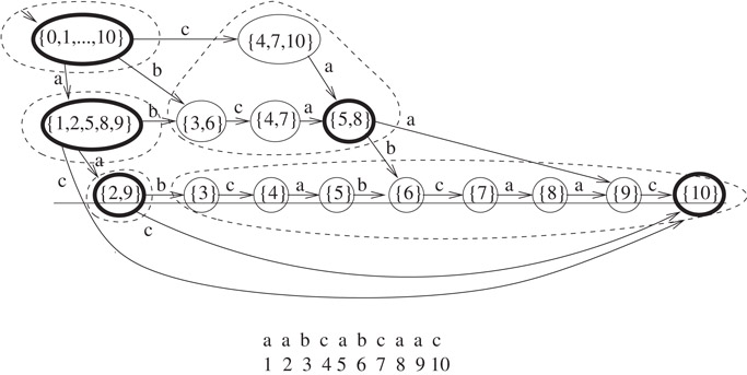
Figure 31.8Partition of nodes into groups with the same prime implicant.
Lemma 31.7
A right-equivalence class is nonprime if and only if it has exactly one outgoing edge in the DAWG.
We now describe how to obtain the compact DAWG from the DAWG in linear time. For ease of presentation, we describe how to carry it out in four depth-first traversals of the DAWG. However, in practice, only two depth-first traversals are required, since the operations of the first three traversals can be carried out during a single depth-first traversal.
In the first depth-first traversal, we may label each class with a single position from its set of ending positions. This is done in postorder: when retreating from a node, copy its label from the label of any of its successors, which have already been labeled, and subtract 1 from it.
By Lemma 31.7, the prime implicant of a class is the class itself if it is prime; otherwise, it is the unique successor that is prime. Let the distance to its prime implicant be the length of this unique path.
In postorder during the second traversal, we may label each node with a pointer to its prime implicant and label this pointer with the distance to the prime implicant. If the class C is a sink or has more than one outgoing edge, this is just a pointer from C to itself with distance label 0. Otherwise, C has a unique successor D, which is already labeled with a pointer to D’s prime implicant A with distance label i. Label C with a pointer to A with distance label i + 1.
In the third traversal, we install the compact DAWG edges. If we label the edges explicitly with their string labels, we will exceed linear time and storage. Instead, we may take advantage of the fact that the label of every edge is a substring of t. We label each edge with the length of its label (see Figure 31.9). When retreating from a prime node B during the traversal, for each DAWG edge (BC) out of B, let D be C’s prime implicant, let i be the distance of D from C. Install a compact DAWG edge from B to D that has length label i + 1.

Figure 31.9Representing the edge labels of the compact DAWG (cf. Figure 31.2) Each edge label is a substring of t with end positions at the end position labels of the principal nodes. The label of the edge can therefore be represented implicitly by labeling each node with one member of its position set, and labeling each edge with the length of its label. For instance, the edge labeled 3 from the source to the node labeled “5” is labeled with the substring of length 3 that ends at position 5, hence, the one occupying positions 3, 4, and 5 of the text. Since the text can be randomly accessed, the text can be used to look up the label of the edge. This ensures that the edge labels take O(|t|) space, since they take O(1) for each node and edge.
On the final traversal, we may remove the DAWG nodes, DAWG edges, and the prime implication pointers.
31.4.1Using the Compact DAWG to Find the Locations of a String in the Text
Let v be a node of the compact DAWG, and let x be the corresponding prime implicant. Let the total length of a path from v to the sink be the sum of the length labels of the edges on the path. Observe that there is a path of total length i from v to the sink iff x has an ending position at n − i + 1.
Lemma 31.8
Let x be a prime substring of t, and let k be the number of occurrences of x in t. Given x’s node in the compact DAWG of t, it takes O(k) time to retrieve the ending positions of x in t.
Proof. Recursively explore all paths out of the node, and whenever the sink is encountered, subtract the total length of the current path from n + 1 and return it.
The running time follows from the following observations. One position is returned for each leaf of the recursion tree; the sets of positions returned by recursive calls are disjoint; and every internal node of the recursion tree has at least two children since every node of the compact DAWG has at least two outgoing edges.■
The representation of Figure 31.9 is therefore just as powerful as that of Figure 31.2: The edge labels are implied by accessing t using the numbers on edges and nodes, while the position labels of the vertices can be retrieved in linear time by the algorithm of Lemma 31.8.
The representation of Figure 31.9 now gives an O(|p| + k) algorithm for finding the k occurrences of a substring p in a text t. One must index into the compact DAWG from the source, matching letters of p with letters of the implicit word labels of the compact edges. If a letter of p cannot be matched, then p does not occur as a subword of t. Otherwise, p is the concatenation of a set of word labels on a path, followed by part of the word label of a final edge (u, v). This takes O(|p|) time. Let i be the number of remaining unmatched letters of the word label of (u, v). The k ending positions of p are given by subtracting i from the k ending positions of v, which can be retrieved in O(k) time using the algorithm of Lemma 31.8.
For instance, using the compact DAWG of Figure 31.2 to find the locations where abc occurs, we match a to the label a of an edge out of the source to the node with position set {1, 2, 5, 8, 9}, then bc to the word label of the edge to the node labeled {5, 8}. Though the node is labeled with the position set in the picture, this position set is not available in the linear-space data structure. Instead, we find two paths of length 2 and 5 from this node to the sink, and subtracting 2 and 5 from n = 10 yields the position set {5, 8}. Then, since one letter in the word label bca remains unmatched, we subtract 1 from each member of {5, 8} to obtain {4, 7}, which is the desired answer.
31.4.2Variations and Applications
In Reference 6, a variation of the compact DAWG is given for a collection {t1, t2, …, tk} of texts and can be used to find the k occurrences of a string p in the texts in O(|p| + k) time.
That paper also gives a symmetric version of the compact DAWG. By the symmetry in the definition of the prime subwords of t, the set of prime subwords of the reversal of t are given by reversing the set of prime subwords of t. The compact DAWG of t and of the reversal of t therefore have essentially the same set of nodes; only the edges are affected by the reversal. The symmetric version has a single set of nodes and two sets of edges, one corresponding to the edges of the compact DAWG of t and one corresponding to the edges of the reversal of t. The utility of this structure as a tool for exploring the subword structure of t is described in the paper.
Another variant occurs when t is a cyclic ordering of characters, rather than a linear one. A string p has an occurrence anywhere where it matches the subword contained in an interval on this cycle. A variant of the DAWG, compact DAWG, and compact symmetric DAWG for retrieving occurrences of subwords for t in this case is given in Reference 6. The paper gives algorithms that have time bounds analogous to those given here.
Variations of landscapes, such as that of Figure 31.6, are explored in Reference 7. They give a graphical display of the structure of repetitions in a text. The suffix tree can be used to find the longest common substring of two texts t1 and t2 efficiently. The paper gives O(|t|h(t)) algorithms that use the DAWG to generate the landscape of t (see Definition 31.2), which can be used to help identify functional units in a genomic sequence. One variation of the landscape explored in the paper inputs two texts t1 and t2, and gives a graphical display of the number of occurrences of every substring of t1 in t2, which has obvious applications to the study of evolutionary relationships among organisms.
Mehta and Sahni give a generalization of the compact DAWG and the compact symmetric DAWG to circular sequences is given in Reference 8, and give techniques for analyzing and displaying the structure of strings using the compact symmetric DAWG in References 9 and 10.
We now give a data structure that gives much simpler algorithms, at a cost of slightly increasing the worst-case time required for a query. The algorithms can easily be programmed by undergraduate data structure students.
The data structure is a trie and has one node for each position in the text. The data structures and algorithms can be modified to give the same bounds for construction and searching, but this undermines the principal advantages, which are simplicity and low memory requirements.
The data structure is closely related to trees that are used for storing hash keys in Reference 11.
31.5.1Building the Position Heap
Let a string be represented by a trie if it is the label of a path from the root in the trie.
For analyzing the position heap we adopt the convention of indexing the characters of t in descending order, so . In this case, we let t[i : j] denote .
The algorithm for constructing the position heap can be described informally as follows. The positions of t are visited from right to left as a trie is built. At each position i, a new substring z is added to the set of words represented by the trie. To do this, the longest prefix t[i : j] of t[i : 1] that is already represented in the trie is found by indexing into the trie from the root, using the leading letters of t[i : 1], until one can advance no further. A leaf child of the last node of this path is added, and the edge to it is labeled ti + 1.
The procedure, PHBuild, is given in Algorithm 31.3. Figure 31.10 gives an illustration.

Figure 31.10Construction of the position heap with PHBuild (see Algorithm 31.3). The solid edges reflect the recursively constructed position heap for the suffix t[9 : 1] of t. To get the position heap for t[10 : 1], we use the heap to find the largest prefix bb of t[10 : 1] that is the label of a path in the tree, and add a new child at this spot to record the next larger prefix bba.
Algorithm 31.3
Constructing the Position Heap for a String
PHBuild(t, i)
If i = 1 return a single tree node labeled 1
Else
Recursively construct the position heap H′ for the suffix t[i − 1, 1]
Let t′ = t[i : k] be the maximal prefix of t that is the
label of a path originating at the root in the tree
Let u be the last node of this path
Add a child of u to the tree on edge labeled tk−1, and give it label i
31.5.2Querying the Position Heap
Algorithm 31.4 gives a procedure, PHFind, to find all starting positions of p in t, and Figure 31.11 gives an illustration. The worst-case running time of O(|p|2 + k) to find the k occurrences of p is worse than the O(|p| + k) bound for the suffix tree or DAWG.

Figure 31.11Searching for occurrences of a string in the text t in O(|p|2 + k) time with PHFind (see Algorithm 31.4). How the search is conducted depends on whether the search string is the path label of a node in the position heap. One case is illustrated by search string aba, which is the path label of position 11. The only places where aba may match t are at positions given by ancestors and descendants of t. The descendants {11, 15} do not need to be verified, but the proper ancestors {1, 3, 6} must be verified against t at those positions. Of these, only 3 and 6 are matches. The algorithm returns {3, 6, 11, 15}. The other case is illustrated by baba, which is not the path label of a node. Indexing on it yields position 7 and path label bab ≠ baba. Only the ancestors {2, 5, 7} are candidates, and they must be verified against t. Of these, only 7 is a match. The algorithm returns {7}. Since the ancestor positions occur on the search path, there are O(|p|) of them, and each takes O(|p|) time to verify each of them against t. Descendants can be more numerous, but take O(1) time apiece to retrieve and return, since they do not need to be verified.
Algorithm 31.4
Find All Places in a Text t Where a Substring p Occurs, Given the Position Heap H for t
PHFind (p, t, H)
Let p′ be the maximal prefix of p that is the label of a path P′ from the root of H
S1 be the set of position labels in P′
Let S2 be the subset of S1 that are the positions of occurrences of p in t
If p′ ≠ p then let S3 be the empty set
Else let S3 be the position labels of descendants of the last node of P′
Return S2 ∪ S3
Lemma 31.9
PHFind returns all positions where p occurs in t.
Proof. Let p = p1p2…pm and let . Suppose that i is a position in t where p does not occur. Then i ∉ S2. Any node u with position label i has a path label that is a prefix of t[i : 1]. Since p is not a prefix of this string, it is not a prefix of the path label of u, so i ∉ S3. We conclude that i is not among the positions returned by PHFind.
Next, let h be the position of an occurrence of p. Let x = p[1 : j] be the maximal prefix of p that is represented in the position heap of t[h − 1 : 1], where j = 0 if x = λ. If x ≠ p, then PHBuild created a node with position label h and path label xpj + 1. This is a prefix of p, so h ∈ S1, and, since p occurs at position h, h ∈ S2. If x = p, let y = t[h : k] be the largest prefix of t[h : 1] that is active in t[h − 1 : 1]. Then PHBuild created a node with position label h and path label ytk − 1, and h ∈ S3. In either case, h is returned as a position where P occurs.■
Lemma 31.10
PHFind takes O(|p|2 + k) worst-case time to return the k occurrences of p in t.
Proof. The members of S3 can be retrieved in O(1) time apiece using a depth-first traversal of the subtree rooted at the last node on path P′. Since all nodes of S1 occur on a path whose label is a prefix of p, there are at most m + 1 members of S1. Checking them against t to see which are members of S2 takes O(|p|) time apiece, for a total of O(|p|2) time in the worst case.■
This time bound overstates what can be expected in practice, since, in most cases, the string is known to match on a prefix, but there is no reason to expect that it will be similar to the position that it is supposed to match in the region beyond this prefix. A good heuristic is to match the string from the end, rather than from the beginning, since the string has a prefix that is already known to match at the position. Checking to see whether a string matches at a given position will usually require examining one or two characters, discovering a mismatch, and rejecting the string.
Lemma 31.11
PHBuild takes O(|t|h(tR)) time.
Proof. If P = (v0, v1, …, vk) be a path from the root v0 in the position heap, let P1 = (v0, v1, …, v⌊k/2⌋), and let be the remainder of the path. Let i be the position label of vk, and let h′(i) denote the length of the maximum prefix x of t[i : 1] that occurs at least |x| times in t. The path label y of P1 has an occurrence at the position labels of each of its descendants, including those on P2, of which there are at least |y|. Therefore, |y| = O(h′(i)). The time spend by the algorithm at position i of t is proportional to the length of P, which is O(|y|). Therefore, the time spent by the algorithm adding the node for position i is O(h′(i)), hence the time to build the whole heap is by Definition 31.2.■
As with the O(|t|h(t)) algorithm for building the DAWG, this time bound is a practical one in most settings, since h(t) is relatively insensitive to long repeated strings or localized areas of the string with many repetitions. Only strings where most areas of the string are repeated many times elsewhere have high values of h(t), and h(t) can be expected to behave like an O(log n) function in most settings.
31.5.4Improvements to the Time Bounds
In this section, we given an algorithm for constructing the position heap to O(|t|). We also sketch an approach for finding the occurrences of a string p in t to O(|p| + k) using position heaps. Each of these has trade-off costs, such as having greater space requirements and being harder to understand.
The position heap has a dual, which we may call the dual heap (see Figure 31.12). They have the same node set: a node has path label x in the heap iff its path label in the dual is the reversal xR of x. We will refer to the position heap as the primal heap when we wish to contrast it to the dual.

Figure 31.12The position heap and the dual heap of the string abbabbb. The node set of both heaps is the same, but the label of the path leading to a node in the dual heap is the reverse of the label of the path leading to it in the position heap.
It is tempting to think that the dual is just the position heap of the reversal tR of t, but this is not the case. As in the primal heap, the rightmost positions of t are near the root of the dual, but in the primal heap of tR, the leftmost positions of t are near the root. In the primal heap of tR the heap order is inverted, which affects the shape of the tree. Neither the primal nor the dual heap of t is necessarily isomorphic to the primal or dual heap of tR.
Algorithm 31.5
Construct the Position Heap H and its Dual D for a String t[i : 1]. Return (H, D, y), Where y Is a Pointer to the Node with Position Label i.
FastPHBuild (T, i)
If i = 1, return a single tree node labeled 1
Let (H′, D′, v) = FastPHBuild(t, i − 1)
Search upward from v in H′ to find the lowest ancestor v′ of v that has
a child u on edge labeled ti in the dual
Let w be the penultimate node on this path
Let d = dw be the depth of w in the heap
Create a new child y of u in the position heap on edge labeled ti−d
Make y be the child of w in the dual on edge labeled ti
Give y position label i
Give y depth label dy = d + 1
Return the modified position heap, the modified dual, and y
For PHBuild, the bottleneck is finding the node u whose path label is . The dual heap allows us to carry out this step more efficiently. We get an O(|t|) time bound for constructing the position heap by simultaneously constructing the position heap and its dual. It is also necessary to label each node v with its depth dv during construction, in addition to its position label, pv. This gives a compact representation of the path label of v if v is not the root: it is t[pv : pv − dv + 1].
During construction, the primal edges are directed from child to parent, while the dual edges are directed from parent to child. The modified procedure, FastPHBuild, is given in Algorithm 31.5.
Lemma 31.12
FastPHBuild is correct.
Proof. The path label of v is t[i − 1 : i − 1 − dv + 1] = t[i − 1 : i − dv]. Let d = dw be the depth of w. Since w is an ancestor of v, its path label is a prefix of this, so w’s path label is t[i − 1 : i − d]. Since v′ is the parent of w, the path label of v′ is the next shorter prefix, t[i − 1 : i − d + 1]. The path label of v′ in the dual is the reversal of this, and since u is reachable on the dual edge out of v′ that is labeled ti, the path label of u is the reversal of t[i : i − d + 1] in the dual, hence t[i : i − d + 1] in the primal heap. Since w has no child labeled ti in the dual, there is no node whose path label in the dual is the reversal of t[i : i − d], hence no node whose path label is t[i : i − d] in the primal heap.
Therefore, u has path label t[i : i − d + 1] and has no child in the primal graph on ti − d. It follows that updating the primal heap to reflect t[i : 1] requires adding a new child y labeled to u in the primal heap. Since w’s path label is the longest proper suffix of y’s path label, w must be the parent of y in the dual. Since its depth is one greater than w’s, dy = d + 1.■
Lemma 31.13
FastPHBuild takes O(|t|) time.
Proof. The inductive step takes O(1) time, except for the cost of searching upward from v to find v′. Let k be the distance from v′ to v and let k′ = k − 1. The cost of searching upward is O(k). The depth of the new node y is dv′ + 2, so it is dv − k + 2 ≤ dv + 1. Since v is the node added just before y, the depth of each successive node added increases by at most one and decreases by Θ(k). The total increases are O(|t|), so the sum of k’s overall recursive calls is bounded by this, hence also O(|t|).■
On tests we have run on several megabyte texts, FastPHBuild is noticeably faster than PHBuild. This advantage must be weighed against the fact that the algorithm is slightly more difficult to understand and uses more memory during construction, to store the dual edges.
By contrast, the algorithm we describe next for finding the positions of p in t in O(|p| + k) time is unlikely to compete in practice with PHFind, since the worst-case bound of O(|p|2 + k) for PHFind overstates the typical case. However, it is interesting from a theoretical standpoint.
Let # be a character that is not in Σ. Let t#t denote the concatenation of two copies of t with the special character # in between. To obtain the time bound for PHFind, we may build the position heap of t#t in O(|t|) time using FastPHBuild. Index the positions from |t| to −|t| in descending order. This gives 0 as the position of the # character (see Figure 31.13).

Figure 31.13Finding occurrences of p in t in O(|p| + k) time, using a position heap. Because of the extra memory requirements and the good expected performance of the O(|p|2 + k) approach, the algorithm is of theoretical interest only. The trick is to build the position heap of t#t, indexing so that positions in the second occurrence are indexed with negative numbers. To find the occurrences of p in t, it suffices to return only its positive positions in t#t. Indexing into the heap is organized so that positive positions are descendants of nodes that are indexed to. Negative occurrences, which are ancestors, do not need to be verified against the text, eliminating the Θ(|p|2) step of the simpler algorithm.
To find the starting positions of p in t, it suffices to find only its positive starting positions in t#t. Suppose that there is a path labeled p that has at most one node with a positive position number. Finding the last node v of the path takes O(|p|) time, and all k positive starting positions are descendants. We can retrieve them in O(k) time. Since we are not required to find negative position numbers where p occurs, we do not have the Θ(|p|2) cost of finding which ancestors of v are actual matches. This gives an O(|p| + k) bound in this case.
Otherwise, the problem can be solved by chopping p into segments {x1, x2, …, xk} such that each xi is the label of a path from the root in the heap that has exactly one node vi with a positive position number, namely, the last node of the path. Every positive position of xi is matched by a negative position, which must correspond to an ancestor of vi. Since there are at most |xi| ancestors of vi, vi has at most |xi| (positive) descendants, which can be retrieved in O(|xi|) time.
To see that this implies an O(|p|) time bound to return all occurrences of p in t, the reader should first note that a family of k sets X1, X2, …, Xk of integers are represented with sorted lists, it takes O(|X1| + |X2| + … |Xk|) time to find their intersection. The key to this insight is that when two sets in are merged, replacing them with their intersection, the sum of cardinalities of sets in drops by an amount proportional to the time to perform the intersection. Therefore, the bound for all intersections is proportional to the sum of cardinalities of the initial lists. The problem of finding the occurrences of p reduces to this one as follows. Let Xi denote the positive positions of segment xi of p. Shift these positions to the left by |x1x2…xi−1| to find the candidate positions they imply for the left endpoint of p in t. Intersecting the sets of candidates gives the locations of p in t.
To find the substrings {x1, x2, …, xk} of p, index from the root of the position heap on the leading characters of p until a positive node is reached. The label of this path is x1, and recursing on the remaining suffix of p gives {x2, x3, …, xk − 1}. It doesn’t give xk, since an attempt to produce xk in this way it may run out of characters of p before a node with a positive position number is reached. Instead, find xk by indexing from the right end of p using the dual heap until a positive position number is reached. Therefore, {x1, x2, …, xk − 1} represent disjoint intervals p, while xk − 1 and xk can represent overlapping intervals of p. The sum of their lengths is therefore O(|p|), giving an O(|p|) bound to find all occurrences of p in t in this case.
1.E. M. McCreight. A space-economical suffix tree construction algorithm. Journal of the ACM, 23:262–272, 1976.
2.U. Manber and E. Myers. Suffix arrays a new method for on-line search. SIAM Journal of Computing, 22:935–948, 1993.
3.G. Kucherov. On-line construction of position heaps. Journal of Discrete Algorithms, 20:3–11, 2013.
4.Y. Nakamura, I. Tomohiro, S. Inenaga, and H. Bannai. Constructing LZ78 tries and position heaps in linear time for large alphabets. Information Processing Letters, 115:655–659, 2015.
5.Y. Nakamura, S. Inenaga, H. Bannai, and M. Takaheda. The position heap of a trie. Lecture Notes in Computer Science, 7608:360–371, 2012.
6.A. Blumer, J. Blumer, D. Ehrenfeucht, D. Haussler, and R. McConnell. Complete inverted files for efficient text retrieval and analysis. Journal of the ACM, 34:578–595, 1987.
7.B. Clift, D. Haussler, R. McConnell, T. D. Schneider, and G. D. Stormo. Sequence landscapes. Nucleic Acids Research, 14:141–158, 1986.
8.D. P. Mehta and S. Sahni. A data structure for circular string analysis and visualization. IEEE Transactions on Computers, 42:992–997, 1993.
9.D. P. Mehta and S. Sahni. Computing display conflicts in string visualization. IEEE Transactions on Computers, 43:350–361, 1994.
10.D. P. Mehta and S. Sahni. Models, techniques, and algorithms for finding, selecting and displaying patterns in strings and other discrete objects. Journal of Systems and Software, 39:201–221, 1997.
11.E. G. Coffman and J. Eve. File structures using hashing functions. Communications of the ACM, 11:13–21, 1981.