
Sartaj Sahni
University of Florida
A Simple Computer Model•Effect of Cache Misses on Run Time•Matrix Multiplication
Big Oh Notation (O)•Omega(Ω) and Theta (Θ) Notations•Little Oh Notation (o)
Substitution Method•Table-Lookup Method
What Is Amortized Complexity?•Maintenance Contract•The McWidget Company•Subset Generation
The topic “Analysis of Algorithms” is concerned primarily with determining the memory (space) and time requirements (complexity) of an algorithm. Since the techniques used to determine memory requirements are a subset of those used to determine time requirements, in this chapter, we focus on the methods used to determine the time complexity of an algorithm.
The time complexity (or simply, complexity) of an algorithm is measured as a function of the problem size. Some examples are given below.
1.The complexity of an algorithm to sort n elements may be given as a function of n.
2.The complexity of an algorithm to multiply an m × n matrix and an n × p matrix may be given as a function of m, n, and p.
3.The complexity of an algorithm to determine whether x is a prime number may be given as a function of the number, n, of bits in x. Note that n = ⌈log2(x + 1)⌉.
We partition our discussion of algorithm analysis into the following sections.
1.Operation counts
2.Step counts
3.Counting cache misses
4.Asymptotic complexity
5.Recurrence equations
6.Amortized complexity
7.Practical complexities
See [1–4] for additional material on algorithm analysis.
One way to estimate the time complexity of a program or method is to select one or more operations, such as add, multiply, and compare, and to determine how many of each is done. The success of this method depends on our ability to identify the operations that contribute most to the time complexity.
Example 1.1
[Max Element] Figure 1.1 gives an algorithm that returns the position of the largest element in the array a[0:n-1]. When n > 0, the time complexity of this algorithm can be estimated by determining the number of comparisons made between elements of the array a. When n ≤ 1, the for loop is not entered. So no comparisons between elements of a are made. When n > 1, each iteration of the for loop makes one comparison between two elements of a, and the total number of element comparisons is n-1. Therefore, the number of element comparisons is max{n-1, 0}. The method max performs other comparisons (e.g., each iteration of the for loop is preceded by a comparison between i and n) that are not included in the estimate. Other operations such as initializing positionOfCurrentMax and incrementing the for loop index i are also not included in the estimate.

Figure 1.1Finding the position of the largest element in a[0:n-1].
The algorithm of Figure 1.1 has the nice property that the operation count is precisely determined by the problem size. For many other problems, however, this is not so. Figure 1.2 gives an algorithm that performs one pass of a bubble sort. In this pass, the largest element in a[0:n-1] relocates to position a[n-1]. The number of swaps performed by this algorithm depends not only on the problem size n but also on the particular values of the elements in the array a. The number of swaps varies from a low of 0 to a high of n − 1.

Figure 1.2A bubbling pass.
Since the operation count isn’t always uniquely determined by the problem size, we ask for the best, worst, and average counts.
Example 1.2
[SEQUENTIAL SEARCH] Figure 1.3 gives an algorithm that searches a[0:n-1] for the first occurrence of x. The number of comparisons between x and the elements of a isn’t uniquely determined by the problem size n. For example, if n = 100 and x = a[0], then only 1 comparison is made. However, if x isn’t equal to any of the a[i]s, then 100 comparisons are made.
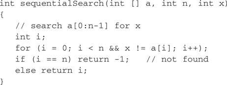
Figure 1.3Sequential search.
A search is successful when x is one of the a[i]s. All other searches are unsuccessful. Whenever we have an unsuccessful search, the number of comparisons is n. For successful searches the best comparison count is 1, and the worst is n. For the average count assume that all array elements are distinct and that each is searched for with equal frequency. The average count for a successful search is
Example 1.3
[Insertion into a Sorted Array] Figure 1.4 gives an algorithm to insert an element x into a sorted array a[0:n-1].
We wish to determine the number of comparisons made between x and the elements of a. For the problem size, we use the number n of elements initially in a. Assume that n ≥ 1. The best or minimum number of comparisons is 1, which happens when the new element x

Figure 1.4Inserting into a sorted array.
is to be inserted at the right end. The maximum number of comparisons is n, which happens when x is to be inserted at the left end. For the average assume that x has an equal chance of being inserted into any of the possible n+1 positions. If x is eventually inserted into position i+1 of a, i ≥ 0, then the number of comparisons is n-i. If x is inserted into a[0], the number of comparisons is n. So the average count is
This average count is almost 1 more than half the worst-case count.
The operation-count method of estimating time complexity omits accounting for the time spent on all but the chosen operations. In the step-count method, we attempt to account for the time spent in all parts of the algorithm. As was the case for operation counts, the step count is a function of the problem size.
A step is any computation unit that is independent of the problem size. Thus 10 additions can be one step; 100 multiplications can also be one step; but n additions, where n is the problem size, cannot be one step. The amount of computing represented by one step may be different from that represented by another. For example, the entire statement
return a+b+b*c+(a+b-c)/(a+b)+4;
can be regarded as a single step if its execution time is independent of the problem size. We may also count a statement such as
x = y;
as a single step.
To determine the step count of an algorithm, we first determine the number of steps per execution (s/e) of each statement and the total number of times (i.e., frequency) each statement is executed. Combining these two quantities gives us the total contribution of each statement to the total step count. We then add the contributions of all statements to obtain the step count for the entire algorithm.
Example 1.4
[Sequential Search] Tables 1.1 and 1.2 show the best- and worst-case step-count analyses for sequentialSearch (Figure 1.3).
Table 1.1Best-Case Step Count for Figure 1.3
|
Statement |
s/e |
Frequency |
Total Steps |
|
|
0 |
0 |
0 |
|
|
0 |
0 |
0 |
|
|
1 |
1 |
1 |
|
|
1 |
1 |
1 |
|
|
1 |
1 |
1 |
|
|
1 |
1 |
1 |
|
|
0 |
0 |
0 |
|
Total |
4 |
Table 1.2Worst-Case Step Count for Figure 1.3
|
Statement |
s/e |
Frequency |
Total Steps |
|
|
0 |
0 |
0 |
|
|
0 |
0 |
0 |
|
|
1 |
1 |
1 |
|
|
1 |
n + 1 |
n + 1 |
|
|
1 |
1 |
1 |
|
|
1 |
0 |
0 |
|
|
0 |
0 |
0 |
|
Total |
n + 3 |
For the average step-count analysis for a successful search, we assume that the n values in a are distinct and that in a successful search, x has an equal probability of being any one of these values. Under these assumptions the average step count for a successful search is the sum of the step counts for the n possible successful searches divided by n. To obtain this average, we first obtain the step count for the case x = a[j] where j is in the range [0, n − 1] (see Table 1.3).
Table 1.3Step Count for Figure 1.3 When x = a[j]
|
Statement |
s/e |
Frequency |
Total Steps |
|
|
0 |
0 |
0 |
|
|
0 |
0 |
0 |
|
|
1 |
1 |
1 |
|
|
1 |
j + 1 |
j + 1 |
|
|
1 |
1 |
1 |
|
|
1 |
1 |
1 |
|
|
0 |
0 |
0 |
|
Total |
j + 4 |
Now we obtain the average step count for a successful search:
This value is a little more than half the step count for an unsuccessful search.
Now suppose that successful searches occur only 80% of the time and that each a[i] still has the same probability of being searched for. The average step count for sequentialSearch is
0.8 ∗ (average count for successful searches) + 0.2 ∗ (count for an unsuccessful search)
= 0.8(n + 7)/2 + 0.2(n + 3)
= 0.6n + 3.4
Traditionally, the focus of algorithm analysis has been on counting operations and steps. Such a focus was justified when computers took more time to perform an operation than they took to fetch the data needed for that operation. Today, however, the cost of performing an operation is significantly lower than the cost of fetching data from memory. Consequently, the run time of many algorithms is dominated by the number of memory references (equivalently, number of cache misses) rather than by the number of operations. Hence, algorithm designers focus on reducing not only the number of operations but also the number of memory accesses. Algorithm designers focus also on designing algorithms that hide memory latency.
Consider a simple computer model in which the computer’s memory consists of an L1 (level 1) cache, an L2 cache, and main memory. Arithmetic and logical operations are performed by the arithmetic and logic unit (ALU) on data resident in registers (R). Figure 1.5 gives a block diagram for our simple computer model.

Figure 1.5A simple computer model.
Typically, the size of main memory is tens or hundreds of megabytes; L2 cache sizes are typically a fraction of a megabyte; L1 cache is usually in the tens of kilobytes; and the number of registers is between 8 and 32. When you start your program, all your data are in main memory.
To perform an arithmetic operation such as an add, in our computer model, the data to be added are first loaded from memory into registers, the data in the registers are added, and the result is written to memory.
Let one cycle be the length of time it takes to add data that are already in registers. The time needed to load data from L1 cache to a register is two cycles in our model. If the required data are not in L1 cache but are in L2 cache, we get an L1 cache miss and the required data are copied from L2 cache to L1 cache and the register in 10 cycles. When the required data are not in L2 cache either, we have an L2 cache miss and the required data are copied from main memory into L2 cache, L1 cache, and the register in 100 cycles. The write operation is counted as one cycle even when the data are written to main memory because we do not wait for the write to complete before proceeding to the next operation. For more details on cache organization, see [5].
1.4.2Effect of Cache Misses on Run Time
For our simple model, the statement a = b + c is compiled into the computer instructions
load a; load b; add; store c;
where the load operations load data into registers and the store operation writes the result of the add to memory. The add and the store together take two cycles. The two loads may take anywhere from 4 cycles to 200 cycles depending on whether we get no cache miss, L1 misses, or L2 misses. So the total time for the statement a = b + c varies from 6 cycles to 202 cycles. In practice, the variation in time is not as extreme because we can overlap the time spent on successive cache misses.
Suppose that we have two algorithms that perform the same task. The first algorithm does 2000 adds that require 4000 load, 2000 add, and 2000 store operations and the second algorithm does 1000 adds. The data access pattern for the first algorithm is such that 25% of the loads result in an L1 miss and another 25% result in an L2 miss. For our simplistic computer model, the time required by the first algorithm is 2000 ∗ 2 (for the 50% loads that cause no cache miss) + 1000 ∗ 10 (for the 25% loads that cause an L1 miss) + 1000 ∗ 100 (for the 25% loads that cause an L2 miss) + 2000 ∗ 1 (for the adds) + 2000 ∗ 1 (for the stores) = 118,000 cycles. If the second algorithm has 100% L2 misses, it will take 2000 ∗ 100 (L2 misses) + 1000 ∗ 1 (adds) + 1000 ∗ 1 (stores) = 202,000 cycles. So the second algorithm, which does half the work done by the first, actually takes 76% more time than is taken by the first algorithm.
Computers use a number of strategies (such as preloading data that will be needed in the near future into cache, and when a cache miss occurs, the needed data as well as data in some number of adjacent bytes are loaded into cache) to reduce the number of cache misses and hence reduce the run time of a program. These strategies are most effective when successive computer operations use adjacent bytes of main memory.
Although our discussion has focused on how cache is used for data, computers also use cache to reduce the time needed to access instructions.
The algorithm of Figure 1.6 multiplies two square matrices that are represented as two-dimensional arrays. It performs the following computation:
c[i][j]=n∑k=1a[i][k]∗b[k][j],1≤i≤n,1≤j≤n |
(1.1) |
|---|

Figure 1.6Multiply two n × n matrices.
Figure 1.7 is an alternative algorithm that produces the same two-dimensional array c as is produced by Figure 1.6. We observe that Figure 1.7 has two nested for loops that are not present in Figure 1.6 and does more work than is done by Figure 1.6 with respect to indexing into the array c. The remainder of the work is the same.

Figure 1.7Alternative algorithm to multiply square matrices.
You will notice that if you permute the order of the three nested for loops in Figure 1.7, you do not affect the result array c. We refer to the loop order in Figure 1.7 as ijk order. When we swap the second and third for loops, we get ikj order. In all, there are 3! = 6 ways in which we can order the three nested for loops. All six orderings result in methods that perform exactly the same number of operations of each type. So you might think all six take the same time. Not so. By changing the order of the loops, we change the data access pattern and so change the number of cache misses. This in turn affects the run time.
In ijk order, we access the elements of a and c by rows; the elements of b are accessed by column. Since elements in the same row are in adjacent memory and elements in the same column are far apart in memory, the accesses of b are likely to result in many L2 cache misses when the matrix size is too large for the three arrays to fit into L2 cache. In ikj order, the elements of a, b, and c are accessed by rows. Therefore, ikj order is likely to result in fewer L2 cache misses and so has the potential to take much less time than taken by ijk order.
For a crude analysis of the number of cache misses, assume we are interested only in L2 misses; that an L2 cache-line can hold w matrix elements; when an L2 cache-miss occurs, a block of w matrix elements is brought into an L2 cache line; and that L2 cache is small compared to the size of a matrix. Under these assumptions, the accesses to the elements of a, b and c in ijk order, respectively, result in n3/w, n3, and n2/w L2 misses. Therefore, the total number of L2 misses in ijk order is n3(1 + w + 1/n)/w. In ikj order, the number of L2 misses for our three matrices is n2/w, n3/w, and n3/w, respectively. So, in ikj order, the total number of L2 misses is n3(2 + 1/n)/w. When n is large, the ration of ijk misses to ikj misses is approximately (1 + w)/2, which is 2.5 when w = 4 (e.g., when we have a 32-byte cache line and the data is double precision) and 4.5 when w = 8 (e.g., when we have a 64-byte cache line and double-precision data). For a 64-byte cache line and single-precision (i.e., 4 byte) data, w = 16 and the ratio is approximately 8.5.
Figure 1.8 shows the normalized run times of a Java version of our matrix multiplication algorithms. In this figure, mult refers to the multiplication algorithm of Figure 1.6. The normalized run time of a method is the time taken by the method divided by the time taken by ikj order.

Figure 1.8Normalized run times for matrix multiplication.
Matrix multiplication using ikj order takes 10% less time than does ijk order when the matrix size is n = 500 and 16% less time when the matrix size is 2000. Equally surprising is that ikj order runs faster than the algorithm of Figure 1.6 (by about 5% when n = 2000). This despite the fact that ikj order does more work than is done by the algorithm of Figure 1.6.
Let p(n) and q(n) be two nonnegative functions. p(n) is asymptotically bigger (p(n) asymptotically dominates q(n)) than the function q(n) iff
limn→∞q(n)p(n)=0 |
(1.2) |
|---|
q(n) is asymptotically smaller than p(n) iff p(n) is asymptotically bigger than q(n). p(n) and q(n) are asymptotically equal iff neither is asymptotically bigger than the other.
In the following discussion the function f(n) denotes the time or space complexity of an algorithm as a function of the problem size n. Since the time or space requirements of a program are nonnegative quantities, we assume that the function f has a nonnegative value for all values of n. Further, since n denotes an instance characteristic, we assume that n ≥ 0. The function f(n) will, in general, be a sum of terms. For example, the terms of f(n) = 9n2 + 3n + 12 are 9n2, 3n, and 12. We may compare pairs of terms to determine which is bigger. The biggest term in the example f(n) is 9n2.
Example 1.5
Since
3n2 + 2n + 6 is asymptotically bigger than 10n + 7 and 10n + 7 is asymptotically smaller than 3n2 + 2n + 6. A similar derivation shows that 8n4 + 9n2 is asymptotically bigger than 100n3 − 3, and that 2n2 + 3n is asymptotically bigger than 83n. 12n + 6 is asymptotically equal to 6n + 2.
Figure 1.9 gives the terms that occur frequently in a step-count analysis. Although all the terms in Figure 1.9 have a coefficient of 1, in an actual analysis, the coefficients of these terms may have a different value.
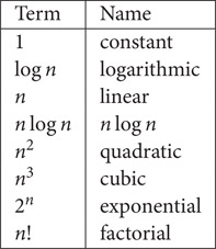
Figure 1.9Commonly occurring terms.
We do not associate a logarithmic base with the functions in Figure 1.9 that include log n because for any constants a and b greater than 1, logan = logbn/ logba. So logan and logbn are asymptotically equal.
The definition of asymptotically smaller implies the following ordering for the terms of Figure 1.9 (< is to be read as “is asymptotically smaller than”):
Asymptotic notation describes the behavior of the time or space complexity for large instance characteristics. Although we will develop asymptotic notation with reference to step counts alone, our development also applies to space complexity and operation counts.
The notation f(n) = O(g(n)) (read as “f(n) is big oh of g(n)”) means that f(n) is asymptotically smaller than or equal to g(n). Therefore, in an asymptotic sense g(n) is an upper bound for f(n).
Example 1.6
From Example 1.5, it follows that 10n + 7 = O(3n2 + 2n + 6); 100n3 − 3 = O(8n4 + 9n2). We see also that 12n + 6 =O(6n + 2); 3n2 + 2n + 6 ≠ O(10n + 7); and 8n4 + 9n2 ≠ O(100n3 − 3).
Although Example 1.6 uses the big oh notation in a correct way, it is customary to use g(n) functions that are unit terms (i.e., g(n) is a single term whose coefficient is 1) except when f(n) = 0. In addition, it is customary to use, for g(n), the smallest unit term for which the statement f(n) = O(g(n)) is true. When f(n) = 0, it is customary to use g(n) = 0.
Example 1.7
The customary way to describe the asymptotic behavior of the functions used in Example 1.6 is 10n + 7 = O(n); 100n3 − 3 = O(n3); 12n + 6 = O(n); 3n2 + 2n + 6 ≠ O(n); and 8n4 + 9n2 ≠ O(n3).
In asymptotic complexity analysis, we determine the biggest term in the complexity; the coefficient of this biggest term is set to 1. The unit terms of a step-count function are step-count terms with their coefficients changed to 1. For example, the unit terms of 3n2 + 6n log n + 7n + 5 are n2, n log n, n, and 1; the biggest unit term is n2. So when the step count of a program is 3n2 + 6n log n + 7n + 5, we say that its asymptotic complexity is O(n2).
Notice that f(n) = O(g(n)) is not the same as O(g(n)) = f(n). In fact, saying that O(g(n)) = f(n) is meaningless. The use of the symbol = is unfortunate, as this symbol commonly denotes the equals relation. We can avoid some of the confusion that results from the use of this symbol (which is standard terminology) by reading the symbol = as “is” and not as “equals.”
1.5.2Omega (Ω) and Theta (Θ) Notations
Although the big oh notation is the most frequently used asymptotic notation, the omega and theta notations are sometimes used to describe the asymptotic complexity of a program.
The notation f(n) = Ω(g(n)) (read as “f(n) is omega of g(n)”) means that f(n) is asymptotically bigger than or equal to g(n). Therefore, in an asymptotic sense, g(n) is a lower bound for f(n). The notation f(n) = Θ(g(n)) (read as “f(n) is theta of g(n)”) means that f(n) is asymptotically equal to g(n).
Example 1.8
10n + 7 = Ω(n) because 10n + 7 is asymptotically equal to n; 100n3 − 3 = Ω(n3); 12n + 6 = Ω(n); 3n3 + 2n + 6 = Ω(n); 8n4 + 9n2 = Ω(n3); 3n3 + 2n + 6 ≠ Ω(n5); and 8n4 + 9n2 ≠ Ω(n5).
10n + 7 = Θ(n) because 10n + 7 is asymptotically equal to n; 100n3 − 3 = Θ(n3); 12n + 6 = Θ(n); 3n3 + 2n + 6 ≠ Θ(n); 8n4 + 9n2 ≠ Θ(n3); 3n3 + 2n + 6 ≠ Θ(n5); and 8n4 + 9n2 ≠ Θ(n5).
The best-case step count for sequentialSearch (Figure 1.3) is 4 (Table 1.1), the worst-case step count is n + 3, and the average step count is 0.6n + 3.4. So the best-case asymptotic complexity of sequentialSearch is Θ(1), and the worst-case and average complexities are Θ(n). It is also correct to say that the complexity of sequentialSearch is Ω(1) and O(n) because 1 is a lower bound (in an asymptotic sense) and n is an upper bound (in an asymptotic sense) on the step count.
When using the Ω notation, it is customary to use, for g(n), the largest unit term for which the statement f(n) = Ω(g(n)) is true.
At times it is useful to interpret O(g(n)), Ω(g(n)), and Θ(g(n)) as being the following sets:
O(g(n)) = {f(n)|f(n) = O(g(n))}
Ω(g(n)) = {f(n)|f(n) = Ω(g(n))}
Θ(g(n)) = {f(n)|f(n) = Θ(g(n))}
Under this interpretation, statements such as O(g1(n)) = O(g2(n)) and Θ(g1(n)) = Θ(g2(n)) are meaningful. When using this interpretation, it is also convenient to read f(n) = O(g(n)) as “f of n is in (or is a member of) big oh of g of n” and so on.
The little oh notation describes a strict upper bound on the asymptotic growth rate of the function f. f(n) is little oh of g(n) iff f(n) is asymptotically smaller than g(n). Equivalently, f(n) = o(g(n)) (read as “f of n is little oh of g of n”) iff f(n) = O(g(n)) and f(n) ≠ Ω(g(n)).
Example 1.9
[LITTLE OH] 3n + 2 = o(n2) as 3n + 2 = O(n2) and 3n + 2 ≠ Ω(n2). However, 3n + 2 ≠ o(n). Similarly, 10n2+ 4n+2 = o(n3), but is not o(n2).
The little oh notation is often used in step-count analyses. A step count of 3n + o(n) would mean that the step count is 3n plus terms that are asymptotically smaller than n. When performing such an analysis, one can ignore portions of the program that are known to contribute less than Θ(n) steps.
Recurrence equations arise frequently in the analysis of algorithms, particularly in the analysis of recursive as well as divide-and-conquer algorithms.
Example 1.10
[BINARY SEARCH] Consider a binary search of the sorted array a[l : r], where n = r − l + 1 ≥ 0, for the element x. When n = 0, the search is unsuccessful and when n = 1, we compare x and a[l]. When n > 1, we compare x with the element a[m] (m = ⌊(l + r)/2⌋) in the middle of the array. If the compared elements are equal, the search terminates; if x < a[m], we search a[l : m − 1]; otherwise, we search a[m + 1 : r]. Let t(n) be the worst-case complexity of binary search. Assuming that t(0) = t(1), we obtain the following recurrence.
t(n)={t(1)n≤1t(⌊n/2⌋)+cn>1 |
(1.3) |
|---|
where c is a constant.
Example 1.11
[MERGE SORT] In a merge sort of a[0 : n − 1], n ≥ 1, we consider two cases. When n = 1, no work is to be done as a one-element array is always in sorted order. When n > 1, we divide a into two parts of roughly the same size, sort these two parts using the merge sort method recursively, then finally merge the sorted parts to obtain the desired sorted array. Since the time to do the final merge is Θ(n) and the dividing into two roughly equal parts takes O(1) time, the complexity, t(n), of merge sort is given by the recurrence:
t(n)={t(1)n=1t(⌊n/2⌋)+t(⌈n/2⌉)+cnn>1 |
(1.4) |
|---|
where c is a constant.
Solving recurrence equations such as Equations 1.3 and 1.4 for t(n) is complicated by the presence of the floor and ceiling functions. By making an appropriate assumption on the permissible values of n, these functions may be eliminated to obtain a simplified recurrence. In the case of Equations 1.3 and 1.4 an assumption such as n is a power of 2 results in the simplified recurrences:
t(n)={t(1)n≤1t(n/2)+cn>1 |
(1.5) |
|---|
and
t(n)={t(1)n=12t(n/2)+cnn>1 |
(1.6) |
|---|
Several techniques—substitution, table lookup, induction, characteristic roots, and generating functions—are available to solve recurrence equations. We describe only the substitution and table lookup methods.
In the substitution method, recurrences such as Equations 1.5 and 1.6 are solved by repeatedly substituting right-side occurrences (occurrences to the right of =) of t(x), x > 1, with expressions involving t(y), y < x. The substitution process terminates when the only occurrences of t(x) that remain on the right side have x = 1.
Consider the binary search recurrence of Equation 1.5. Repeatedly substituting for t() on the right side, we get
For the merge sort recurrence of Equation 1.6, we get
The complexity of many divide-and-conquer algorithms is given by a recurrence of the form
t(n)={t(1)n=1a∗t(n/b)+g(n)n>1 |
(1.7) |
|---|
where a and b are known constants. The merge sort recurrence, Equation 1.6, is in this form. Although the recurrence for binary search, Equation 1.5, isn’t exactly in this form, the n ≤ 1 may be changed to n = 1 by eliminating the case n = 0. To solve Equation 1.7, we assume that t(1) is known and that n is a power of b (i.e., n = bk). Using the substitution method, we can show that
t(n)=nlogba[t(1)+f(n)] |
(1.8) |
|---|
where f(n) = ∑kj=1h(bj) and h(n) = g(n)/nlogba.
Table 1.4 tabulates the asymptotic value of f(n) for various values of h(n). This table allows us to easily obtain the asymptotic value of t(n) for many of the recurrences we encounter when analyzing divide-and-conquer algorithms.
Table 1.4f(n) Values for Various h(n) Values
|
h(n) |
f(n) |
|
O(nr), r < 0 |
O(1) |
|
Θ((log n)i), i ≥ 0 |
Θ(((log n)i+1)/(i + 1)) |
|
Ω(nr), r > 0 |
Θ(h(n)) |
Let us solve the binary search and merge sort recurrences using this table. Comparing Equation 1.5 with n ≤ 1 replaced by n = 1 with Equation 1.7, we see that a = 1, b = 2, and g(n) = c. Therefore, logb(a) = 0, and h(n) = g(n)/nlogba = c = c (log n)0 = Θ(( log n)0). From Table 1.4, we obtain f(n) = Θ( log n). Therefore, t(n) = nlogba(c + Θ( log n))= Θ ( log n).
For the merge sort recurrence, Equation 1.6, we obtain a = 2, b = 2, and g(n) = cn. So logba = 1 and h(n) = g(n)/n = c = Θ((log n)0). Hence f(n) = Θ( log n) and t(n) = n(t(1) + Θ( log n)) = Θ(n log n).
1.7.1What Is Amortized Complexity?
The complexity of an algorithm or of an operation such as an insert, search, or delete, as defined in Section 1.1, is the actual complexity of the algorithm or operation. The actual complexity of an operation is determined by the step count for that operation, and the actual complexity of a sequence of operations is determined by the step count for that sequence. The actual complexity of a sequence of operations may be determined by adding together the step counts for the individual operations in the sequence. Typically, determining the step count for each operation in the sequence is quite difficult, and instead, we obtain an upper bound on the step count for the sequence by adding together the worst-case step count for each operation.
When determining the complexity of a sequence of operations, we can, at times, obtain tighter bounds using amortized complexity rather than worst-case complexity. Unlike the actual and worst-case complexities of an operation which are closely related to the step count for that operation, the amortized complexity of an operation is an accounting artifact that often bears no direct relationship to the actual complexity of that operation. The amortized complexity of an operation could be anything. The only requirement is that the sum of the amortized complexities of all operations in the sequence be greater than or equal to the sum of the actual complexities. That is
∑1≤i≤namortized(i)≥∑1≤i≤nactual(i) |
(1.9) |
|---|
where amortized(i) and actual(i), respectively, denote the amortized and actual complexities of the ith operation in a sequence of n operations. Because of this requirement on the sum of the amortized complexities of the operations in any sequence of operations, we may use the sum of the amortized complexities as an upper bound on the complexity of any sequence of operations.
You may view the amortized cost of an operation as being the amount you charge the operation rather than the amount the operation costs. You can charge an operation any amount you wish so long as the amount charged to all operations in the sequence is at least equal to the actual cost of the operation sequence.
Relative to the actual and amortized costs of each operation in a sequence of n operations, we define a potential function P(i) as below
P(i)=amortized(i)−actual(i)+P(i−1) |
(1.10) |
|---|
That is, the ith operation causes the potential function to change by the difference between the amortized and actual costs of that operation. If we sum Equation 1.10 for 1 ≤ i ≤ n, we get
or
or
From Equation 1.9, it follows that
P(n)−P(0)≥0 |
(1.11) |
|---|
When P(0) = 0, the potential P(i) is the amount by which the first i operations have been overcharged (i.e., they have been charged more than their actual cost).
Generally, when we analyze the complexity of a sequence of n operations, n can be any nonnegative integer. Therefore, Equation 1.11 must hold for all nonnegative integers.
The preceding discussion leads us to the following three methods to arrive at amortized costs for operations:
1.Aggregate Method
In the aggregate method, we determine an upper bound for the sum of the actual costs of the n operations. The amortized cost of each operation is set equal to this upper bound divided by n. You may verify that this assignment of amortized costs satisfies Equation 1.9 and is, therefore, valid.
2.Accounting Method
In this method, we assign amortized costs to the operations (probably by guessing what assignment will work), compute the P(i)s using Equation 1.10, and show that P(n) − P(0) ≥ 0.
3.Potential Method
Here, we start with a potential function (probably obtained using good guess work) that satisfies Equation 1.11 and compute the amortized complexities using Equation 1.10.
1.7.2.1Problem Definition
In January, you buy a new car from a dealer who offers you the following maintenance contract: $50 each month other than March, June, September and December (this covers an oil change and general inspection), $100 every March, June, and September (this covers an oil change, a minor tune-up, and a general inspection), and $200 every December (this covers an oil change, a major tune-up, and a general inspection). We are to obtain an upper bound on the cost of this maintenance contract as a function of the number of months.
1.7.2.2Worst-Case Method
We can bound the contract cost for the first n months by taking the product of n and the maximum cost incurred in any month (i.e., $200). This would be analogous to the traditional way to estimate the complexity–take the product of the number of operations and the worst-case complexity of an operation. Using this approach, we get $200n as an upper bound on the contract cost. The upper bound is correct because the actual cost for n months does not exceed $200n.
1.7.2.3Aggregate Method
To use the aggregate method for amortized complexity, we first determine an upper bound on the sum of the costs for the first n months. As tight a bound as is possible is desired. The sum of the actual monthly costs of the contract for the first n months is
The amortized cost for each month is set to $75. Table 1.5 shows the actual costs, the amortized costs, and the potential function value (assuming P(0) = 0) for the first 16 months of the contract.
Table 1.5Maintenance Contract

Notice that some months are charged more than their actual costs and others are charged less than their actual cost. The cumulative difference between what the operations are charged and their actual costs is given by the potential function. The potential function satisfies Equation 1.11 for all values of n. When we use the amortized cost of $75 per month, we get $75n as an upper bound on the contract cost for n months. This bound is tighter than the bound of $200n obtained using the worst-case monthly cost.
1.7.2.4Accounting Method
When we use the accounting method, we must first assign an amortized cost for each month and then show that this assignment satisfies Equation 1.11. We have the option to assign a different amortized cost to each month. In our maintenance contract example, we know the actual cost by month and could use this actual cost as the amortized cost. It is, however, easier to work with an equal cost assignment for each month. Later, we shall see examples of operation sequences that consist of two or more types of operations (e.g., when dealing with lists of elements, the operation sequence may be made up of search, insert, and remove operations). When dealing with such sequences we often assign a different amortized cost to operations of different types (however, operations of the same type have the same amortized cost).
To get the best upper bound on the sum of the actual costs, we must set the amortized monthly cost to be the smallest number for which Equation 1.11 is satisfied for all n. From the above table, we see that using any cost less than $75 will result in P(n) − P(0) < 0 for some values of n. Therefore, the smallest assignable amortized cost consistent with Equation 1.11 is $75.
Generally, when the accounting method is used, we have not computed the aggregate cost. Therefore, we would not know that $75 is the least assignable amortized cost. So we start by assigning an amortized cost (obtained by making an educated guess) to each of the different operation types and then proceed to show that this assignment of amortized costs satisfies Equation 1.11. Once we have shown this, we can obtain an upper bound on the cost of any operation sequence by computing
where k is the number of different operation types and f(i) is the frequency of operation type i (i.e., the number of times operations of this type occur in the operation sequence).
For our maintenance contract example, we might try an amortized cost of $70. When we use this amortized cost, we discover that Equation 1.11 is not satisfied for n = 12 (e.g.) and so $70 is an invalid amortized cost assignment. We might next try $80. By constructing a table such as the one above, we will observe that Equation 1.11 is satisfied for all months in the first 12 month cycle, and then conclude that the equation is satisfied for all n. Now, we can use $80n as an upper bound on the contract cost for n months.
1.7.2.5Potential Method
We first define a potential function for the analysis. The only guideline you have in defining this function is that the potential function represents the cumulative difference between the amortized and actual costs. So, if you have an amortized cost in mind, you may be able to use this knowledge to develop a potential function that satisfies Equation 1.11, and then use the potential function and the actual operation costs (or an upper bound on these actual costs) to verify the amortized costs.
If we are extremely experienced, we might start with the potential function
Without the aid of the table (Table 1.5) constructed for the aggregate method, it would take quite some ingenuity to come up with this potential function. Having formulated a potential function and verified that this potential function satisfies Equation 1.11 for all n, we proceed to use Equation 1.10 to determine the amortized costs.
From Equation 1.10, we obtain amortized(i) = actual(i) + P(i) − P(i − 1). Therefore,
and so on. Therefore, the amortized cost for each month is $75. So, the actual cost for n months is at most $75n.
1.7.3.1Problem Definition
The famous McWidget company manufactures widgets. At its headquarters, the company has a large display that shows how many widgets have been manufactured so far. Each time a widget is manufactured, a maintenance person updates this display. The cost for this update is $c + dm, where c is a fixed trip charge, d is a charge per display digit that is to be changed, and m is the number of digits that are to be changed. For example, when the display is changed from 1399 to 1400, the cost to the company is $c + 3d because 3 digits must be changed. The McWidget company wishes to amortize the cost of maintaining the display over the widgets that are manufactured, charging the same amount to each widget. More precisely, we are looking for an amount $e = amortized(i) that should levied against each widget so that the sum of these charges equals or exceeds the actual cost of maintaining/updating the display ($e ∗ n ≥ actual total cost incurred for first n widgets for all n ≥ 1). To keep the overall selling price of a widget low, we wish to find as small an e as possible. Clearly, e > c + d because each time a widget is made, at least one digit (the least significant one) has to be changed.
1.7.3.2Worst - Case Method
This method does not work well in this application because there is no finite worst-case cost for a single display update. As more and more widgets are manufactured, the number of digits that need to be changed increases. For example, when the 1000th widget is made, 4 digits are to be changed incurring a cost of c + 4d, and when the 1,000,000th widget is made, 7 digits are to be changed incurring a cost of c + 7d. If we use the worst-case method, the amortized cost to each widget becomes infinity.
1.7.3.3Aggregate Method
Let n be the number of widgets made so far. As noted earlier, the least significant digit of the display has been changed n times. The digit in the ten’s place changes once for every ten widgets made, that in the hundred’s place changes once for every hundred widgets made, that in the thousand’s place changes once for every thousand widgets made, and so on. Therefore, the aggregate number of digits that have changed is bounded by
So, the amortized cost of updating the display is $c + d(1.11111…)n/n < c + 1.12d. If the McWidget company adds $c + 1.12d to the selling price of each widget, it will collect enough money to pay for the cost of maintaining the display. Each widget is charged the cost of changing 1.12 digits regardless of the number of digits that are actually changed. Table 1.6 shows the actual cost, as measured by the number of digits that change, of maintaining the display, the amortized cost (i.e., 1.12 digits per widget), and the potential function. The potential function gives the difference between the sum of the amortized costs and the sum of the actual costs. Notice how the potential function builds up so that when it comes time to pay for changing two digits, the previous potential function value plus the current amortized cost exceeds 2. From our derivation of the amortized cost, it follows that the potential function is always nonnegative.
Table 1.6Data for Widgets

1.7.3.4Accounting Method
We begin by assigning an amortized cost to the individual operations, and then we show that these assigned costs satisfy Equation 1.11. Having already done an amortized analysis using the aggregate method, we see that Equation 1.11 is satisfied when we assign an amortized cost of $c + 1.12d to each display change. Typically, however, the use of the accounting method is not preceded by an application of the aggregate method and we start by guessing an amortized cost and then showing that this guess satisfies Equation 1.11.
Suppose we assign a guessed amortized cost of $c + 2d for each display change.
This analysis also shows us that we can reduce the amortized cost of a widget to $c + 1.12d.
An alternative proof method that is useful in some analyses involves distributing the excess charge P(i) − P(0) over various accounting entities, and using these stored excess charges (called credits) to establish P(i + 1) − P(0) ≥ 0. For our McWidget example, we use the display digits as the accounting entities. Initially, each digit is 0 and each digit has a credit of 0 dollars. Suppose we have guessed an amortized cost of $c + (1.111…)d. When the first widget is manufactured, $c + d of the amortized cost is used to pay for the update of the display and the remaining $(0.111…)d of the amortized cost is retained as a credit by the least significant digit of the display. Similarly, when the second through ninth widgets are manufactured, $c + d of the amortized cost is used to pay for the update of the display and the remaining $(0.111…)d of the amortized cost is retained as a credit by the least significant digit of the display. Following the manufacture of the ninth widget, the least significant digit of the display has a credit of $(0.999…)d and the remaining digits have no credit. When the tenth widget is manufactured, $c + d of the amortized cost are used to pay for the trip charge and the cost of changing the least significant digit. The least significant digit now has a credit of $(1.111…)d. Of this credit, $d are used to pay for the change of the next least significant digit (i.e., the digit in the ten’s place), and the remaining $(0.111…)d are transferred to the ten’s digit as a credit. Continuing in this way, we see that when the display shows 99, the credit on the ten’s digit is $(0.999…)d and that on the one’s digit (i.e., the least significant digit) is also $(0.999…)d. When the 100th widget is manufactured, $c+d of the amortized cost are used to pay for the trip charge and the cost of changing the least significant digit, and the credit on the least significant digit becomes $(1.111…)d. Of this credit, $d are used to pay for the change of the ten’s digit from 9 to 0, the remaining $(0.111…)d credit on the one’s digit is transferred to the ten’s digit. The credit on the ten’s digit now becomes $(1.111…)d. Of this credit, $d are used to pay for the change of the hundred’s digit from 0 to 1, the remaining $(0.111…)d credit on the ten’s digit is transferred to the hundred’s digit.
The above accounting scheme ensures that the credit on each digit of the display always equals $(0.111…)dv, where v is the value of the digit (e.g., when the display is 206 the credit on the one’s digit is $(0.666…)d, the credit on the ten’s digit is $0, and that on the hundred’s digit is $(0.222…)d.
From the preceding discussion, it follows that P(n) − P(0) equals the sum of the digit credits and this sum is always nonnegative. Therefore, Equation 1.11 holds for all n.
1.7.3.5Potential Method
We first postulate a potential function that satisfies Equation 1.11, and then use this function to obtain the amortized costs. From the alternative proof used above for the accounting method, we can see that we should use the potential function P(n) = (0.111…)d∑ivi, where vi is the value of the ith digit of the display. For example, when the display shows 206 (at this time n = 206), the potential function value is (0.888…)d. This potential function satisfies Equation 1.11.
Let q be the number of 9 s at the right end of j (i.e., when j = 12903999, q = 3). When the display changes from j to j + 1, the potential change is (0.111…)d(1 − 9q) and the actual cost of updating the display is $c + (q + 1)d. From Equation 1.10, it follows that the amortized cost for the display change is
1.7.4.1Problem Definition
The subsets of a set of n elements are defined by the 2n vectors x[1:n], where each x[i] is either 0 or 1. x[i] = 1 iff the ith element of the set is a member of the subset. The subsets of a set of three elements are given by the eight vectors 000, 001, 010, 011, 100, 101, 110, and 111, for example. Starting with an array x[1:n] has been initialized to zeroes (this represents the empty subset), each invocation of algorithm nextSubset (Figure 1.10) returns the next subset. When all subsets have been generated, this algorithm returns null.

Figure 1.10Subset enumerator.
We wish to determine how much time it takes to generate the first m, 1 ≤ m ≤ 2n subsets. This is the time for the first m invocations of nextSubset.
1.7.4.2Worst-Case Method
The complexity of nextSubset is Θ(c), where c is the number of x[i]s that change. Since all n of the x[i]s could change in a single invocation of nextSubset, the worst-case complexity of nextSubset is Θ(n). Using the worst-case method, the time required to generate the first m subsets is O(mn).
1.7.4.3Aggregate Method
The complexity of nextSubset equals the number of x[i]s that change. When nextSubset is invoked m times, x[n] changes m times; x[n − 1] changes ⌊m/2⌋ times; x[n − 2] changes ⌊m/4⌋ times; x[n − 3] changes ⌊m/8⌋ times; and so on. Therefore, the sum of the actual costs of the first m invocations is ∑0≤i≤⌊log2m⌋(m/2i)<2m. So, the complexity of generating the first m subsets is actually O(m), a tighter bound than obtained using the worst-case method.
The amortized complexity of nextSubset is (sum of actual costs)/m < 2m/m = O(1).
1.7.4.4Accounting Method
We first guess the amortized complexity of nextSubset, and then show that this amortized complexity satisfies Equation 1.11. Suppose we guess that the amortized complexity is 2. To verify this guess, we must show that P(m) − P(0) ≥ 0 for all m.
We shall use the alternative proof method used in the McWidget example. In this method, we distribute the excess charge P(i) − P(0) over various accounting entities, and use these stored excess charges to establish P(i + 1) − P(0) ≥ 0. We use the x[j]s as the accounting entities. Initially, each x[j] is 0 and has a credit of 0. When the first subset is generated, 1 unit of the amortized cost is used to pay for the single x[j] that changes and the remaining 1 unit of the amortized cost is retained as a credit by x[n], which is the x[j] that has changed to 1. When the second subset is generated, the credit on x[n] is used to pay for changing x[n] to 0 in the while loop, 1 unit of the amortized cost is used to pay for changing x[n − 1] to 1, and the remaining 1 unit of the amortized cost is retained as a credit by x[n − 1], which is the x[j] that has changed to 1. When the third subset is generated, 1 unit of the amortized cost is used to pay for changing x[n] to 1, and the remaining 1 unit of the amortized cost is retained as a credit by x[n], which is the x[j] that has changed to 1. When the fourth subset is generated, the credit on x[n] is used to pay for changing x[n] to 0 in the while loop, the credit on x[n − 1] is used to pay for changing x[n − 1] to 0 in the while loop, 1 unit of the amortized cost is used to pay for changing x[n − 2] to 1, and the remaining 1 unit of the amortized cost is retained as a credit by x[n − 2], which is the x[j] that has changed to 1. Continuing in this way, we see that each x[j] that is 1 has a credit of 1 unit on it. This credit is used to pay the actual cost of changing this x[j] from 1 to 0 in the while loop. One unit of the amortized cost of nextSubset is used to pay for the actual cost of changing an x[j] to 1 in the else clause, and the remaining one unit of the amortized cost is retained as a credit by this x[j].
The above accounting scheme ensures that the credit on each x[j] that is 1 is exactly 1, and the credit on each x[j] that is 0 is 0.
From the preceding discussion, it follows that P(m) − P(0) equals the number of x[j]s that are 1. Since this number is always nonnegative, Equation 1.11 holds for all m.
Having established that the amortized complexity of nextSubset is 2 = O(1), we conclude that the complexity of generating the first m subsets equals m ∗ amortized complexity = O(m).
1.7.4.5Potential Method
We first postulate a potential function that satisfies Equation 1.11, and then use this function to obtain the amortized costs. Let P(j) be the potential just after the jth subset is generated. From the proof used above for the accounting method, we can see that we should define P(j) to be equal to the number of x[i]s in the jth subset that are equal to 1.
By definition, the 0th subset has all x[i] equal to 0. Since P(0) = 0 and P(j) ≥ 0 for all j, this potential function P satisfies Equation 1.11. Consider any subset x[1:n]. Let q be the number of 1 s at the right end of x[] (i.e., x[n], x[n − 1], …, x[n − q + 1], are all 1s). Assume that there is a next subset. When the next subset is generated, the potential change is 1 − q because q 1 s are replaced by 0 in the while loop and a 0 is replaced by a 1 in the else clause. The actual cost of generating the next subset is q + 1. From Equation 1.10, it follows that, when there is a next subset, the amortized cost for nextSubset is
When there is no next subset, the potential change is − q and the actual cost of nextSubset is q. From Equation 1.10, it follows that, when there is no next subset, the amortized cost for nextSubset is
Therefore, we can use 2 as the amortized complexity of nextSubset. Consequently, the actual cost of generating the first m subsets is O(m).
We have seen that the time complexity of a program is generally some function of the problem size. This function is very useful in determining how the time requirements vary as the problem size changes. For example, the run time of an algorithm whose complexity is Θ(n2) is expected to increase by a factor of 4 when the problem size doubles and by a factor of 9 when the problem size triples.
The complexity function also may be used to compare two algorithms P and Q that perform the same task. Assume that algorithm P has complexity Θ(n) and that algorithm Q has complexity Θ(n2). We can assert that algorithm P is faster than algorithm Q for “sufficiently large” n. To see the validity of this assertion, observe that the actual computing time of P is bounded from above by cn for some constant c and for all n, n ≥ n1, while that of Q is bounded from below by dn2 for some constant d and all n, n ≥ n2. Since cn ≤ dn2 for n ≥ c/d, algorithm P is faster than algorithm Q whenever n≥max{n1,n2,c/d}.
One should always be cautiously aware of the presence of the phrase sufficiently large in the assertion of the preceding discussion. When deciding which of the two algorithms to use, we must know whether the n we are dealing with is, in fact, sufficiently large. If algorithm P actually runs in 106n milliseconds while algorithm Q runs in n2 milliseconds and if we always have n ≤ 106, then algorithm Q is the one to use.
To get a feel for how the various functions grow with n, you should study Figures 1.11 and 1.12 very closely. These figures show that 2n grows very rapidly with n. In fact, if a algorithm needs 2n steps for execution, then when n = 40, the number of steps needed is approximately 1.1 * 1012. On a computer performing 1,000,000,000 steps per second, this algorithm would require about 18.3 minutes. If n = 50, the same algorithm would run for about 13 days on this computer. When n = 60, about 310.56 years will be required to execute the algorithm, and when n = 100, about 4 ∗ 1013 years will be needed. We can conclude that the utility of algorithms with exponential complexity is limited to small n (typically n ≤ 40).
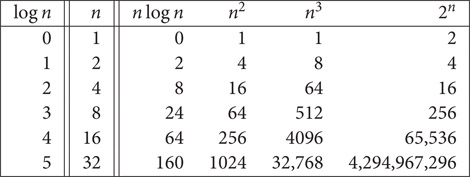
Figure 1.11Value of various functions.

Figure 1.12Plot of various functions.
Algorithms that have a complexity that is a high-degree polynomial are also of limited utility. For example, if an algorithm needs n10 steps, then our 1,000,000,000 steps per second computer needs 10 seconds when n = 10; 3171 years when n = 100; and 3.17 ∗ 1013 years when n = 1000. If the algorithm’s complexity had been n3 steps instead, then the computer would need 1 second when n = 1000, 110.67 minutes when n = 10,000, and 11.57 days when n = 100,000.
Figure 1.13 gives the time that a 1,000,000,000 instructions per second computer needs to execute an algorithm of complexity f(n) instructions. One should note that currently only the fastest computers can execute about 1,000,000,000 instructions per second. From a practical standpoint, it is evident that for reasonably large n (say n > 100) only algorithms of small complexity (such as n, n log n, n2, and n3) are feasible. Further, this is the case even if we could build a computer capable of executing 1012 instructions per second. In this case the computing times of Figure 1.13 would decrease by a factor of 1000. Now when n = 100, it would take 3.17 years to execute n10 instructions and 4 ∗ 1010 years to execute 2n instructions.

Figure 1.13Run times on a 1,000,000,000 instructions per second computer.
This work was supported, in part, by the National Science Foundation under grant CCR-9912395.
1.T. Cormen, C. Leiserson, and R. Rivest, Introduction to Algorithms, McGraw-Hill, New York, NY, 1992.
2.E. Horowitz, S. Sahni, and S. Rajasekaran, Fundamentals of Computer Algorithms, W. H. Freeman and Co., New York, NY, 1998.
3.G. Rawlins, Compared to What: An Introduction to the Analysis of Algorithms, W. H. Freeman and Co., New York, NY, 1992.
4.S. Sahni, Data Structures, Algorithms, and Applications in Java, McGraw-Hill, NY, 2000.
5.J. Hennessey and D. Patterson, Computer Organization and Design, Second Edition, Morgan Kaufmann Publishers, Inc., San Francisco, CA, 1998, Chapter 7.
*This chapter has been reprinted from first edition of this Handbook, without any content updates.