56. Geographic Information Systems

Geographic Information Systems (GISs) serve the purpose of maintaining, analyzing, and visualizing spatial data that represent geographic objects, such as mountains, lakes, houses, roads, and tunnels. For spatial data, geometric (spatial) attributes play a key role, representing, for example, points, lines, and regions in the plane or volumes in three-dimensional space. They model geographical features of the real world, such as geodesic measurement points, boundary lines between adjacent pieces of land (in a cadastral database), trajectories of mobile users, lakes or recreational park regions (in a tourist information system). In three dimensions, spatial data describe tunnels, underground pipe systems in cities, mountain ranges, or quarries. In addition, spatial data in a GIS possess nongeometric, so-called thematic attributes, such as the time when a geodesic measurement was taken, the name of the owner of a piece of land in a cadastral database, the usage history of a park.

This chapter aims to highlight some of the data structures and algorithms aspects of GISs that define challenging research problems, and some that show interesting solutions. More background information and deeper technical expositions can be found in books [1–10].

56.1.1Geometric Objects

Our technical exposition will be limited to geometric objects with a vector representation. Here, a point is described by its coordinates in the Euclidean plane with a Cartesian coordinate system. We deliberately ignore the geographic reality that the earth is (almost) spherical, to keep things simple. A line segment is defined by its two end points. A polygonal line is a sequence of line segments with coinciding endpoints along the way. A (simple) polygonal region is described by its corner points, in clockwise (or counterclockwise) order around its interior. In contrast, in a raster representation of a region, each point in the region, discretized at some resolution, has an individual representation, just like a pixel in a raster image. Satellites take raster images at an amazing rate, and hence raster data abound in GISs, challenging current storage technology with terabytes of incoming data per day. Nevertheless, we are not concerned with raster images in this chapter, even though some of the techniques that we describe have implications for raster data [11]. The reason for our choice is the different flavor that operations with raster images have, as compared with vector data, requiring a chapter of their own.

56.1.2Topological versus Metric Data

For some purposes, not even metric information is needed; it is sufficient to model the topology of a spatial dataset. How many states share a border with Iowa? is an example of a question of this topological type. In this chapter, however, we will not specifically study the implications that this limitation has. There is a risk of confusing the limitation to topological aspects only with the explicit representation of topology in the data structure. Here, the term explicit refers to the fact that a topological relationship need not be computed with substantial effort. As an example, assume that a partition of the plane into polygons is stored so that each polygon individually is a separate clockwise sequence of points around its interior. In this case, it is not easy to find the polygons that are neighbors of a given polygon, that is, share some boundary. If, however, the partition is stored so that each edge of the polygon explicitly references both adjacent polygons (just like the doubly connected edge list in computational geometry [12]), then a simple traversal around the given polygon will reveal its neighbors. It will always be an important design decision for a data structure which representation to pick.

56.1.3Geometric Operations

Given this range of applications and geometric objects, it is no surprise that a GIS is expected to support a large variety of operations. We will discuss a few of them now, and then proceed to explain in detail how to perform two fundamental types of operations in the remainder of the chapter, spatial searching and spatial join. Spatial searching refers to rather elementary geometric operations without which no GIS can function. Here are a few examples, always working on a collection of geometric objects, such as points, lines, polygonal lines, or polygons. A nearest neighbor query for a query point asks for an object in the collection that is closest to the query point, among all objects in the collection. A distance query for a query point and a certain distance asks for all objects in the collection that are within the given distance from the query point. A range query (or window query) for a query range asks for all objects in the collection that intersect the given orthogonal window. A ray shooting query for a point and a direction asks for the object in the collection that is hit first if the ray starts at the given point and shoots in the given direction. A point-in-polygon query for a query point asks for all polygons in the collection in which the query point lies. These five types of queries are illustrations only; many more query types are just as relevant. For a more extensive discussion on geometric operations, see the chapters on geometric data structures in this Handbook. In particular, it is well understood that great care must be taken in geometric computations to avoid numeric problems, because already tiny numerical inaccuracies can have catastrophic effects on computational results. Practically all books on geometric computation devote some attention to this problem [12–14], and geometric software libraries such as CGAL [15] take care of the problem by offering exact geometric computation.

56.1.4Geometric Data Structures

Naturally, we can only hope to respond to queries of this nature quickly, if we devise and make use of appropriate data structures. An extra complication arises here due to the fact that GISs maintain data sets too large for internal memory. So far, GIS have also not been designed for large distributed computer networks that would allow to exploit the internal memory of many nodes as it is known from the recently emerged Big Data technologies [16]. Data maintenance and analysis operations on a central system can therefore be efficient only if they take external memory properties into account, as discussed also in other chapters in this Handbook. We will limit ourselves here to external storage media with direct access to storage blocks, such as disks and flash memory. A block access to a random block on disk takes time to move the read–write–head to the proper position (the latency), and then to read or write the data in the block (the transfer). With today’s disks, where block sizes are on the order of several kilobytes, latency is a few milliseconds, and transfer time is less by a factor of about 100. Therefore, it pays to read a number of blocks in consecution, because they require the head movement only once, and in this way amortize its cost over more than one block. We will discuss in detail how to make use of this cost savings possibility.

All of the above geometric operations (see Section 56.1.3) on an external memory geometric data structure follow the general filter-refinement pattern [17] that first, all relevant blocks are read from disk. This step is a first (potentially rough) filter that makes a superset of the relevant set of geometric objects available for processing in main memory. In a second step, a refinement identifies the exact set of relevant objects. Even though complicated geometric operators can make this refinement step quite time-consuming, in this chapter we limit our considerations to the filter step. Because queries are the dominant operations in GISs by far, we do not explicitly discuss updates (see the chapters on external memory spatial data structures in this Handbook for more information).

56.1.5Applications of Geographic Information

Before we go into technical detail, let us mention a few of the applications that make GISs a challenging research area up until today, with more fascinating problems to expect than what we can solve.

56.1.5.1Map Overlay

Maps are the most well-known visualizations of geographical data. In its simplest form, a map is a partition of the plane into simple polygons. Each polygon may represent, for instance, an area with a specific thematic attribute value. For the attribute land use, polygons can stand for forest, savanna, lake areas in a simplistic example, whereas for the attribute state, polygons represent Arizona, New Mexico, Texas. In a GIS, each separable aspect of the data (such as the planar polygonal partitions just mentioned) is said to define a layer. This makes it easy to think about certain analysis and viewing operations, by just superimposing (overlaying) layers or, more generally, by applying Boolean operations on sets of layers. In our example, an overlay of a land use map with a state map defines a new map, where each new polygon is (some part of) the intersection of two given polygons, one from each layer. In map overlay in general, a Boolean combination of all involved thematic attributes together defines polygons of the resulting map, and one resulting attribute value in our example is the savannas of Texas. Map overlay has been studied in many different contexts, ranging from the special case of convex polygons in the partition and an internal memory plane-sweep computation [18] to the general case that we will describe in the context of spatial join processing later in this chapter.

56.1.5.2Map Labeling

Map visualization is an entire field of its own (traditionally called cartography), with the general task to layout a map in such a way that it provides just the information that is desired, no more and no less; one might simply say, the map looks right. What that means in general is hard to say. For maps with texts that label cities, rivers, and the like, looking right implies that the labels are in proper position and size, that they do not run into each other or into important geometric features, and that it is obvious to which geometric object a label refers. Many simply stated problems in map labeling turn out to be NP-hard to solve exactly, and as a whole, map labeling is an active research area with a variety of unresolved questions (see Reference 19 for a tutorial introduction). In particular, the boundary-labeling problem [20] has attracted research attention assuming that labels are placed around an iso-oriented rectangle that contains a set of point objects. Dynamic map labeling [21] is another recently addressed problem of maps that are generated in an ad hoc manner using a set of operations such as zooming and panning. The underlying goal is to preserve a consistent layout of the labels among source and target maps.

56.1.5.3Cartographic Generalization

If cartographers believe that automatically labeled maps will never look really good, they believe even more that another aspect that plays a role in map visualization will always need human intervention, namely map generalization. Generalization of a map is the process of reducing the complexity and contents of a map by discarding less important information and retaining the more essential characteristics. This is most prominently used in producing a map at a low resolution, given a map at a high resolution. Generalization ensures that the reader of the produced low resolution map is not overwhelmed with all the details from the high resolution map, displayed in small size in a densely filled area. Generalization is viewed to belong to the art of map making, with a whole body of rules of its own that can guide the artist [22,23]. The collection [24] provides a summary of the various flavors of generalization. Nevertheless, computational solutions of some subproblem help a lot, such as the simplification of a high resolution polygonal line to a polygonal line with fewer corner points that does not deviate too much from the given line. For line simplification, old algorithmic ideas [25] have seen efficient implementations [26]. A survey and an extensive experimental comparison of various algorithms is given in Reference 27 in terms of positional accuracy and processing time. Interesting extensions of the classical problem exist with the goal of preserving topological consistency [24,28].

Maps on demand, with a selected viewing window, to be shown on a screen with given resolution, imply the choice of a corresponding scale and therefore need the support of data structures that allow the retrieval up to a desired degree of detail [29]. More recently, van Oosterom and Meijers [30] have proposed a vario-scale structure that supports a continuous generalization while preserving consistency [110]. Apart from the simplest aspects, automatic map generalization, access support and labeling [21] are still open problems.

56.1.5.4Road Maps

Maps have been used for ages to plan trips. Hence, we want networks of roads, railways, and the like to be represented in a GIS, in addition to the data described earlier. This fits naturally with the geometric objects that are present in a GIS in any case, such as polygonal lines. A point where polygonal lines meet (a node) can then represent an intersection of roads (edges), with a choice which road to take as we move along. The specialty in storing roads comes from the fact that we want to be able to find paths between nodes efficiently, for instance in car navigation systems, while we are driving. The fact that not all roads are equally important can be expressed by weights on the edges. Because a shortest path computation is carried out as a breadth first search on the edge weighted graph, in one way or another (e.g., bidirectional), it makes sense to partition the graph into pages so as to minimize the weight of edges that cross the cuts induced by the partition. Whenever we want to maintain road data together with other thematic data, such as land use data, it also makes sense to store all the data in one structure, instead of using an extra structure for the road network. It may come as no surprise that for some data structures, partitioning the graph and partitioning the other thematic aspects go together very well (compromising a little on both sides), while for others this is not easily the case. The compromise in partitioning the graph does almost no harm, because it is NP-complete to find the optimum partition, and hence a suboptimal solution of some sort is all we can get anyway. An excellent recent survey on road networks and algorithms for shortest-paths can be found in Reference 31. It does not only provide a concise summary of various methods for different problem settings but also contains a very detailed experimental evaluation in terms of multiple factors such as query time, preprocessing cost, and space usage.

56.1.5.5Spatiotemporal Data

Just like for many other database applications, a time component brings a new dimension to spatial data (even in the mathematical sense of the word, if you wish). How did the forest areas in New Mexico develop over the last 20 years? Questions like this one demonstrate that for environmental information systems, a specific branch of GISs, keeping track of developments over time is a must. Spatiotemporal database research is concerned with all problems that the combination of space with time raises, from models and languages, all the way through data structures and query algorithms, to architectures and implementations of systems [32]. In this chapter, we refrain from the temptation to discuss spatiotemporal data structures in detail; see Chapter 23 for an introduction into this lively field.

56.1.5.6Data Mining

The development of spatial data over time is interesting not only for explicit queries but also for data mining. Here, one tries to find relevant patterns in the data, without knowing beforehand the character of the pattern (for an introduction to the field of data mining, see Reference 4). For more advanced topics, the reader is referred to Reference 33. Let us briefly look at a historic example for spatial data mining. A London epidemiologist identified a water pump as the centroid of the locations of cholera cases, and after the water pump was shut down, the cholera subsided. This and other examples are described in Reference 9. If we want to find patterns in quite some generality, we need a large data store that keeps track of data extracted from different data sources over time, a so-called data warehouse. It remains as an important, challenging open problem to efficiently run a spatial data warehouse and mine the spatial data. The spatial nature of the data seems to add the extra complexity that comes from the high autocorrelation present in typical spatial data sets, with the effect that most knowledge discovery techniques today perform poorly. This omnipresent tendency for data to cluster in space has been stated nicely [34]: Everything is related to everything else but nearby things are more related than distant things.

Due to the ubiquitous availability of GPS devices and their capability of tracking arbitrary movements, mining algorithms for trajectories have emerged over the last decade [35]. In addition to clustering and classification of trajectories, one of the most challenging spatial mining tasks is to extract behavioral patterns from very large set of trajectories [36]. A typical pattern is to identify sequences of regions, frequently visited by trajectories in a specified order with similar average stays. The work on trajectories differentiates between physical and semantic ones. A physical trajectory consists of typical physical measurements, such as position, speed, and acceleration, while a semantic or conceptual trajectory [37] adds annotations to the physical trajectory representing semantically richer patterns that are more relevant to a user. For example, someone might be interested in trajectories with high frequency of stops at touristic points. We refer to a recent survey [38] that gives an excellent summary of mining techniques for semantic trajectories.

56.2Space Filling Curves: Order in Many Dimensions

As explained above, our interest in space filling curves (SFCs) comes from two sources. The first one is the fact that we aim at exploiting the typical database support mechanisms that a conventional database management system (DBMS) offers, such as support for transactions and recovery. On the data structures level, this support is automatic if we resort to a data structure that is inherently supported by a DBMS. These days, this is the case for a number of one-dimensional data structures, such as those of the B-tree family (see Chapter 16). In addition, spatial DBMS support one of a small number of multidimensional data structures, such as those of the R-tree family (see Chapter 22) or of a grid-based structure. The second reason for our interest in SFCs is the general curiosity in the gap between one dimension and many: In what way and to what degree can we bridge this gap for the sake of supporting spatial operations of the kind described above? In our setting, the gap between one dimension and many goes back to the lack of a linear order in many dimensions that is useful for all purposes. An SFC tries to overcome this problem at least to some degree, by defining an artificial linear order on a regular grid that is as useful as possible for the intended purpose. Limiting ourselves in this section to two-dimensional space, we define an SFC more formally as a bijective mapping p from an index pair of a grid cell to its number in the linear order:

p : N \times N ⟶ {1, \dots, N^{2}} .

$p : N \times N ⟶ {1, \dots, N^{2}} .$

For the sake of simplicity, we limit ourselves to numbers N = 2n for some positive integer n.

Our main attention is on the choice of the linear order in such a way that range queries are efficient. In the GIS setting, it is not worst-case efficiency that counts, but efficiency in expectation. It is, unfortunately, hard to say what queries can be expected. Therefore, a number of criteria are conceivable according to which the quality of an SFC should be measured. Before entering the discussion about these criteria, let us present some of the most prominent SFCs that have been investigated for GIS data structures.

56.2.1Recursively Defined SFCs

Two SFCs have been investigated most closely for the purpose of producing a linear ordering suitable for data structures for GIS, the z-curve, by some also called Peano curve or Morton encoding, and the Hilbert curve. We depict them in Figures 56.1 and 56.2. They can both be defined recursively with a simple refinement rule. To obtain a 2^{n + 1} × 2^{n + 1} grid from a 2n × 2n grid, replace each cell by the elementary pattern of four cells as in Figure 56.1, with the appropriate rotation for the Hilbert curve, as indicated in Figure 56.2 for the four by four grid (i.e., for n = 2). In the same way, a slightly less popular SFC can be defined, the Gray code curve (see Figure 56.3).

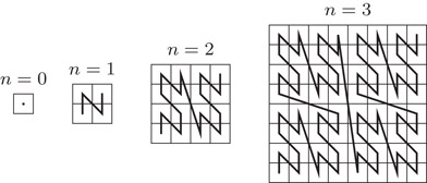
Figure 56.1The z-curve for a 2n × 2n grid, for n = 0,…, 3.

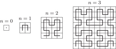
Figure 56.2The Hilbert curve for a 2n × 2n grid, for n = 0,…, 3.

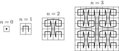
Figure 56.3The Gray curve for a 2n × 2n grid, for n = 0,…, 3.

For all recursively defined SFCs, there is an obvious way to compute the mapping p (and also its inverse), namely just along the recursive definition. Any such computation therefore takes time proportional to the logarithm of the grid size. Without going to great lengths in explaining how this computation is carried out in detail (refer [39] for this and other mathematical aspects of SFCs), let us just mention that there is a particularly nice way of viewing it for the z-curve: Here, p simply alternately interleaves the bits of both of its arguments, when these are expressed in binary. This may have made the z-curve popular among geographers at an early stage, even though our subsequent discussion will reveal that it is not necessarily the best choice.

56.2.2Range Queries for SFC Data Structures

An SFC defines a linear order that is used to store the geographical data objects. We distinguish between two extreme storage paradigms that can be found in spatial data structures, namely a partition of the data space according to the objects present in the data set (such as in R-trees or in B-trees for a single dimension), or a partition of the space only, regardless of the objects (such as in regular cell partitions). The latter makes sense if the distribution of objects is somewhat uniform (see the spatial data structures chapters in this Handbook), and in this case achieves considerable efficiency. Naturally, a multitude of data structures that operate in between both extremes have been proposed, such as the grid file (see the spatial data structures chapters in this Handbook). As to the objects, let us limit ourselves to points in the plane, so that we can focus on a single partition of the plane into grid cells and need not worry about objects that cross cell boundaries (these are dealt with elsewhere in this Handbook, see, e.g., the chapter on R-trees or the survey chapter). For simplicity, let us restrict our attention to partitions of the data space into a 2n × 2n grid, for some integer n. Partitions into other numbers of grid cells (i.e., not powers of 4) can be achieved dynamically for some data structures (see, e.g., z-Hashing [40]), but are not always easy to obtain; we will ignore that aspect for now.

Corresponding to both extreme data structuring principles, there are two ways to associate data with external storage blocks for SFCs. The simplest way is to identify a grid cell with a disk block. This is the usual setting. Grid cell numbers correspond to physical disk block addresses, and a range query translates into the need to access the corresponding set of disk blocks. In the example of Figure 56.4, for instance, the dark query range results in the need to read disk blocks corresponding to cells with numbers 2–3, 6, 8–12, 14, that is, cell numbers come in four consecutive sequences. In the best case, the cells to be read have consecutive numbers, and hence a single disk seek operation will suffice, followed by a number of successive block read operations. In the worst case, the sequence of disk cell numbers to be read breaks into a large number of consecutive pieces. It is one concern in the choice of an SFC to bound this number or some measure related to it (see the next subsection).

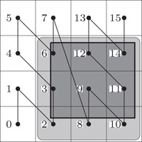
Figure 56.4Range queries and disk seek operations.

The association of a grid cell with exactly one disk block gives a data structure based on an SFC very little flexibility to adapt to a not so uniform data set. A different and more adaptive way of associating disk blocks with grid cells is based on a partition of the data space into cells so that for each cell, the objects in the cell fit on a disk block (as before), but a disk block stores the union of the sets of objects in a consecutive number of cells. This method has the advantage that relatively sparsely populated cells can go together in one disk block, but has the potential disadvantage that disk block maintenance becomes more complex. Not too complex, though, because a disk block can simply be maintained as a node of a B-tree (or, more specifically, a leaf, depending on the B-tree variety), with the content of a cell limiting the granularity of the data in the node. Under this assumption, the adaptation of the data structure to a dynamically changing population of data objects simply translates to split and merge operations of B-tree nodes. In this setting, the measure of efficiency for range queries may well be different from the above. One might be interested in running a range query on the B-tree representation, and ignoring (skipping) the contents of retrieved cells that do not contribute to the result. Hence, for a range query to be efficient, the consecutive single piece of the SFC that includes all cells of the query range should not run outside the query range for too long, that is, for too high a number of cells. We will discuss the effect of a requirement of this type on the design of an SFC in more detail below.

Obviously, there are many other ways in which an SFC can be the basis for a spatial data structure, but we will abstain from a more detailed discussion here and limit ourselves to the two extremes described so far.

56.2.3Are All SFCs Created Equal?

Consider an SFC that visits the cells of a grid by visiting next an orthogonal neighbor of the cell just visited. The Hilbert curve is of this orthogonal neighbor type, but the z-curve is not. Now consider a square query region of some fixed (but arbitrary) size, say k by k grid cells, and study the number of consecutive pieces of the SFC that this query region defines (see Figure 56.5 for a range query region of 3 × 3 grid cells that defines three consecutive pieces of a Hilbert curve). We are interested in the average number of curve pieces over all locations of the query range.

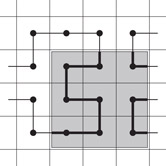
Figure 56.5Disk seeks for an orthogonal curve.

For a fixed location of the query range, the number of curve pieces that the range defines is half the number of orthogonal neighbor links that cross the range boundary (ignoring the starting or ending cell of the entire curve). The reason is that when we start at the first cell of the entire curve and follow the curve, it is an orthogonal neighbor on the curve that leads into the query range and another one that leads out, repeatedly until the query range is exhausted. To obtain the average number of curve pieces per query range, we sum the number of boundary crossing orthogonal neighbors over all query range locations (and then divide that number by twice the number of locations, but this step is of no relevance in our argument).

This sum, however, amounts to the same as summing up for every orthogonal neighbor link the number of range query locations in which it is a crossing link. We content ourselves for the sake of simplicity with an approximate average, by ignoring cells close to the boundary of the data space, an assumption that will introduce only a small inaccuracy whenever k is much less than N (and this is the only interesting case). Hence, each orthogonal link will be a crossing link for 2k query range positions, namely k positions for the query range on each of both sides. The interesting observation now is that this summation disregards the position of the orthogonal link completely (apart from the fact that we ignore an area of size O(kN) along the boundary of the universe). Hence, for any square range query, the average number of pieces of an SFC in the query range is the same across all SFCs of the orthogonal neighbor type.

In this sense, therefore, all SFCs of the orthogonal neighbor type have the same quality. This includes snake like curves such as row-major zigzag snakes and spiral snakes. Orthogonal neighbors are not a painful limitation here: If we allow for other than orthogonal neighbors, this measure of quality can become only worse, because a nonorthogonal neighbor is a crossing link for more query range locations. In rough terms, this indicates that the choice of SFC may not really matter that much. Nevertheless, it also shows that the above measure of quality is not perfectly chosen, since it captures the situation only for square query ranges, and that is not fully adequate for GISs. A recent measure of curve quality looks at a contiguous piece of the SFC and divides the area of its bounding box by the area that this piece of the curve covers. The quality of the curve is then the maximum of these ratios, taken over all contiguous pieces of the curve, appropriately called worst-case bounding-box area ratio (WBA) [41]. When instead of the area of the curve, its perimeter is taken as a basis, it needs to be properly normalized to be comparable to the area of the bounding box. When we normalize by pretending the perimeter belongs to a square, we get the ratio between the area of the bounding box and 1/16th of the squared perimeter. This view results in the worst-case bounding-box squared perimeter ratio (WBP) [41] as another quality measure, taking into account how wiggly the SFC is. For quite a few SFCs, WBA and WBP are at least 2, and the Peano curve comes very close to this bound [41]. These are not the only quality measures; for other measures and a thorough discussion of a variety of SFCs (also in higher dimension) and their qualities, see References 41 and 42. High dimension is useful when spatial objects have a high number of descriptive coordinates, such as four coordinates that describe an axis parallel rectangle, but high dimensional SFCs turn out to be far more complex to understand than those in two dimensions [43–45]. In this chapter, we will continue to discuss the basics for two dimensions only.

56.2.4Many Curve Pieces for a Query Range

The properties that recursively definable SFCs entail for spatial data structure design have been studied from a theoretical perspective [46,47]. The performance of square range queries has been studied [46] on the basis that range queries in a GIS can have any size, but are most likely to not deviate from a square shape by too much. Based on the external storage access model in which disk seek and latency time by far dominates the time to read a block, they allow a range query to skip blocks for efficiency’s sake. Skipping a block amounts to reading it in a sequence of blocks, without making use of the information thus obtained. In the example of Figure 56.4, skipping the blocks of cells 4, 5, 7, and 13 leads to a single sequence of the consecutive blocks 2–14. This can obviously be preferable to just reading consecutive sequences of relevant cell blocks only and therefore performing more disk seek operations, provided that the number of skipped blocks is not too large. In an attempt to quantify one against the other, consider a range query algorithm that is allowed to read a linear number of additional cells [46], as compared with those in the query range. It turns out that for square range query regions of arbitrary size and the permission to read at most a linear number of extra cells, each recursive SFC needs at least three disk seek operations in the worst case. While no recursive SFC needs more than four disk seeks in the worst case, none of the very popular recursive SFCs, including the z-curve, the Hilbert curve, and the Gray code curve, can cope with less than four. One can define a recursive SFC that needs only three disk seeks in the worst case [46], and hence the lower and upper bounds match. This result is only a basis for data structure design, though, because its quality criterion is still too far from GIS reality to guide the design of practical SFCs. Nevertheless, this type of fragmentation has been studied in depth for a number of SFCs [48].

Along the same lines, one can refine the cost measure and account explicitly for disk seek cost [47]. For a sufficiently short sequence of cells, it is cheaper to skip them, but as soon as the sequence length exceeds a constant (that is defined by the disk seek cost, relative to the cost of reading a block), it is cheaper to stop reading and perform a disk seek. A refinement of the simple observation from above leads to performance formulas expressed in the numbers of links of the various types that the SFC uses, taking the relative disk seek cost into consideration [47]. It turns out that the local behavior of SFCs can be modeled well by random walks, again perhaps an indication that at least locally, the choice of a particular SFC is not crucial for the performance.

56.2.5One Curve Piece for a Query Range

The second approach described above reads a single consecutive piece of the SFC to respond to a range query, from the lowest numbered cell in the range to the highest numbered. In general, this implies that a high number of irrelevant cells will be read. As we explained above, such an approach can be attractive, because it allows immediately to make use of well-established data structures such as the B-tree, including all access algorithms. We need to make sure, however, that the inefficiency that results from the extra accessed cells remains tolerable. Let us therefore now calculate this inefficiency approximately. To this end, we change our perspective and calculate for any consecutive sequence of cells along the SFC its shape in two-dimensional space. The shape itself may be quite complicated, but for our purpose a simple rectangular bounding box of all grid cells in question will suffice. The example in Figure 56.6 shows a set of 3 and a set of 4 consecutive cells along the curve, together with their bounding boxes (shaded), residing in a corner of a Hilbert curve. Given this example, a simple measure of quality suggests itself: The fewer useless cells we get in the bounding box, the better. A quick thought reveals that this measure is all too crude, because it does not take into consideration that square ranges are more important than skinny ranges. This bias can be taken into account by placing a piece of the SFC into its smallest enclosing square (see the dotted outline of a 3 × 3 square in Figure 56.6 for a bounding square of the 3 cells), and by taking the occupancy (i.e., percentage of relevant cells) of that square as the measure of quality. The question we now face is to bound the occupancy for a given SFC, across all possible pieces of the curve, and further, to find a best possible curve with respect to this bound. For simplicity’s sake, let us again limit ourselves to curves with orthogonal links.

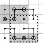
Figure 56.6Bounding a piece of a curve.

Let us first argue that the lower bound on the occupancy, for any SFC, cannot be higher than one-third. This is easy to see by contradiction. Assume to this end that there is an SFC that guarantees an occupancy of more than one-third. In particular, this implies that there cannot be two vertical links immediately after each other, nor can there be two consecutive horizontal links (the reason is that the three cells defining these two consecutive links define a smallest enclosing square of size 3 by 3 cells, with only 3 of these 9 cells being useful, and hence with an occupancy of only one-third). But this finishes the argument, because no SFC can always alternate between vertical and horizontal links (the reason is that a corner of the space that is traversed by the curve makes two consecutive links of the same type unavoidable, see Figure 56.7).

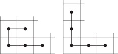
Figure 56.7All possible corner cell traversals (excluding symmetry).

On the positive side, the Hilbert curve guarantees an occupancy of one-third. The reason is that the Hilbert curve gives this guarantee for the 4 × 4 grid, and that this property is preserved in the recursive refinement.

This leads to the conclusion that in terms of the worst-case occupancy guarantee, the Hilbert curve is a best possible basis for a spatial data structure.

56.3Spatial Join

In order to compute map overlays, a GIS provides an operator called spatial join that allows flexible combinations of multiple inputs according to a spatial predicate. The spatial join computes a subset of the Cartesian product of the inputs. Therefore, it is closely related to the join operator of a DBMS. A (binary) join on two sets of spatial objects, say R and S, according to a binary spatial predicate P is given by

S J_{P} (R, S) = {(r, s) | r \in R \land s \in S \land P (r, s)}

$S J_{P} (R, S) = {(r, s) | r \in R \land s \in S \land P (r, s)}$

The join is called a spatial join if the binary predicate P refers to spatial attributes of the objects. Among the most important ones are the following:

•Intersection predicate: P_∩(r, s) = (r ∩ s ≠ ∅).

•Distance predicate: Let DF be a distance function and ε > 0. Then, P_DF (r, s) = (DF(r, s) < ε).

In the following we assume that R and S consist of N two-dimensional spatial objects and that the join returns a total of T pairs of objects. N is assumed being sufficiently large such that the problem cannot be solved entirely in main memory of size M. Therefore, we are particularly interested in external memory algorithms. Due to today’s large main memory, the reader might question this assumption. However, remember that a GIS is a resource-intensive multiuser system where multiple complex queries are running concurrently. Thus the memory assigned to a specific join algorithm might be substantially lower than the total physically available. Given a block size of B, we use the following notations: n = N/B, m = M/B, and t = T/B. Without loss of generality, we assume that B is a divisor of N, M, and T.

A naive approach to processing a spatial join is simply to perform a so-called nested-loop algorithm, which checks the spatial predicate for each pair of objects. The nested-loop algorithm is generally applicable, but requires O(N2) time and O(n2) I/O operations. For special predicates, however, we are able to design new algorithms that provide substantial improvements in runtime compared to the naive approach. Among those is the intersection predicate, which is also the most frequently used predicate in GIS. We therefore will restrict our discussion to the intersection predicate to which the term spatial join will refer to by default. The discussion of other predicates is postponed to the end of the section. We refer to Reference 49 for an excellent survey on spatial joins.

The processing of spatial joins follows the general paradigm of multistep query processing [50] that consists at least of the following two processing steps. In the filter step, a spatial join is performed using conservative approximations of the spatial objects like their minimum bounding rectangles (MBRs). In the refinement step, the candidates of the filter step are checked against the join predicate using their exact geometry. In this section, we limit our discussion on the filter step that utilizes the MBR of the spatial objects. The reader is referred to References 51 and 52 for a detailed discussion of the refinement step and intermediate processing steps that are additionally introduced.

If main memory is large enough to keep R and S entirely in memory, the filter step is (almost) equivalent to the rectangle intersection problem, one of the elementary problems in computational geometry. The problem can be solved in O(N log N + T) runtime where T denotes the size of the output. This can be accomplished by using either a sweep-line algorithm [53] or a divide-and-conquer algorithm [54]. However, the disadvantage of these algorithms is their high overhead that results in a high constant factor. For real-life spatial data, it is generally advisable, see Reference 55 for example, to employ an algorithm that is not optimal in the worst case. The problem of computing spatial joins in main memory has attracted research attention again [56]. In comparison to external algorithms, it has been recognized that performance of main memory solutions is more sensitive to specific implementation details.

56.3.1External Algorithms

In this subsection, we assume that the spatial relations are larger than main memory. According to the availability of indices on both relations, on one of the relations, or on none of the relations, we obtain three different classes of spatial join algorithms for the filter step. This common classification scheme also serves as a foundation in the most recent survey on spatial joins [49].

56.3.1.1Index on Both Spatial Relations

In References 57 and 58, spatial join algorithms were presented where each of the relations is indexed by an R-tree. Starting at the roots, this algorithm synchronously traverses the trees node by node and joins all pairs of overlapping MBRs. If the nodes are leaves, the associated spatial objects are further examined in the refinement step. Otherwise, the algorithm is called recursively for each qualifying pair of entries. As pointed out in Reference 59, this algorithm is not limited to R-trees, but can be applied to a broad class of index structures. Important to both, I/O and CPU cost, is the traversal strategy. In Reference 58, a depth-first strategy was proposed where the qualifying pairs of nodes are visited according to a spatial ordering. If large buffers are available, a breadth-first traversal strategy was shown to be superior [60] in an experimental comparison. Though experimental studies have shown that these algorithms provide fast runtime in practice, the worst-case complexity of the algorithm is O(n2). The general problem of computing an optimal schedule for reading pages from disk is shown [61] to be NP-hard for spatial joins. For specific situations where two arbitrary rectangles from R and S do not share boundaries, the optimal solution can be computed in linear time. This is generally satisfied for bounding boxes of the leaves of R-trees.

56.3.1.2Index on One Spatial Relation

Next, we assume that only one of the relations, say R, is equipped with a spatial index. We distinguish between the following three approaches. The first approach is to issue a range query against the index on R for each MBR of S. By using worst-case optimal spatial index structures, this already results in algorithms with subquadratic runtime. When a page buffer is available, it is also beneficial to sort the MBRs of S according to a criterion that preserves locality, for example, Hilbert value of the center of the MBRs. Then, two consecutive queries will access the same pages with high probability and therefore, the overall number of disk accesses decreases. The second approach as proposed in Reference 62 first creates a spatial index on S, the relation without spatial index. The basic idea for the creation of the index is to use the upper levels of the available index on R as a skeleton. Thereafter, one of the algorithms is applied that requires an index on both of the relations. In Reference 63, an improvement of the algorithm is presented that makes better use of the available main memory. A third approach is presented in References 64 and 65 where the spatial index is used for sorting the data according to one of the minimum boundaries of the rectangles. The sorted sequence then serves as input to an external plane-sweep algorithm.

56.3.1.3Index on None of the Inputs

There are two early proposals on spatial join processing that require no index. The first one [66] suggests using an external version of a computational geometry algorithm. This is basically achieved by employing an external segment tree. The other [17] can be viewed as a sweep-line algorithm where the ordering is derived from z-order. Though the algorithm was originally not designed for rectangles, this can be accomplished in a straightforward manner [67,68]. Like any other sweep-line algorithm, R and S are first sorted, where the z-order serves as criterion in the following way. A rectangle receives the z-value of the smallest cell that still covers the entire rectangle. Let x be a z-value and b(x) = (x0, x1,…, x_k) its binary representation where k = l(x) denotes the level of the corresponding cell. Then, x < _zy, if b(x) < _lexi b(y) where < _lexi denotes the lexicographical order on strings. Note that if x is a prefix of y, x will precede y in lexicographical order. After sorting the input, the processing continues while maintaining a stack for each input. The stacks satisfy the following invariant. The z-value of each element (except the last) is a prefix of its successor. The algorithm simply takes the next element from the sorted inputs, say x from input R. Before x is pushed to the stack, all elements from both stacks are removed that are not prefix of b(x). Thereafter, the entire stack of S is checked for overlap. The worst case of the join occurs when each of the rectangles belongs to the cell that represents the entire data space. Then, the join runs like a nested loop and requires O(n2) I/O operations. This can practically be improved by introducing redundancy [67,69]. However, the worst-case bound remains the same.

Other methods like the Partition Based Spatial-Merge Join (PBSM) [70] and the Spatial Hash-Join [71] are based on the principles of divide-and-conquer where spatial relations are partitioned into buckets that fit into main memory and the join is computed for each pair of corresponding buckets. Let us discuss PBSM in more detail. PBSM performs in four phases. In the first phase, the number of partitions p is computed such that the join for each pair of partitions is likely to be processed in main memory. Then, a grid is introduced with g cells, g ≥ p and each of the cells is then associated with a partition. A rectangle is then assigned to a partition if it intersects with at least one of its cells. In the second phase, pairs of partitions have to be processed that still contain too much data. This usually requires repartitioning of the data into smaller partitions. In the third phase, the join is processed in main memory for every pair of related partitions. The fourth phase consists of sorting, in order to get rid of duplicates in the response set. This however can be replaced by applying an inexpensive check of the result whenever it is produced [72]. Overall, the worst case is O(n2) I/O operations for PBSM.

Spatial Hash-Joins [71] differ from PBSM in the following way. One of the relations is first partitioned using a spatial index structure like an R-tree which uniquely assigns rectangles to leaves, where each of them corresponds to a partition. The other relation is then partitioned using the index of the first relation. Each rectangle has to be stored in all partitions where an overlap with the MBR of the partition exists. Overall, this guarantees the avoidance of duplicate results.

At the end of the 1990s, Arge et al. [55] proposed the first spatial join algorithm that meets the lower I/O bound O(n log_m n + t). The method is an external sweep-line algorithm that is also related to the divide-and-conquer algorithm of Reference 66. Rather than partitioning the problem recursively into two, it is proposed to partition the input recursively into $k = \sqrt{m}$ $k = \sqrt{m}$ strips of almost equal size until the problem is small enough for being solved in memory. This results in a recursion tree of height O(log_m n). At each level, O(m) sorted lists of size Θ(B) are maintained where simultaneously an interval join is performed. Since each of the interval joins runs in O(n′ + t′) (n′ and t′ denote the input size and result size of the join, respectively) and at most O(N) intervals are maintained on each level of the recursion, it follows that at most O(n) accesses are required for each level.

Instead of using the optimal algorithm, Arge et al. [55] employs a plane-sweep algorithm in their experiments where the sweep-line is organized by a dynamic interval tree. This is justified by the observation that the sweep-line is small as it holds only a small fraction of the entire spatial relations. If the algorithm really runs out of memory, it is recommended invoking the optimal algorithm for the entire problem. A different overflow strategy has been presented in Reference 73 where multiple iterations over the spatial relations might be necessary. The advantage of this strategy is that each result element is computed exactly once.

56.3.2Advanced Issues

There are various extensions for spatial joins which are discussed in the following. We first address the processing of spatial joins on multiple inputs. Next, we discuss the processing of distance joins. Eventually, we conclude the section with a brief summary of requirements on the implementation of algorithms within a system.

The problem of joining more than two spatial relations according to a set of binary spatial predicates has been addressed in References 74 and 75. Such a join can be represented by a connected graph where its nodes represent the spatial relations and its edges binary join predicates. A first approach, called pairwise join method (PJM), is to decompose the multiway join into an operator tree of binary joins. The graphs with cycles therefore need to be transformed into a tree by ignoring the edges with lowest selectivity. Depending on the availability of spatial indexes, it is then advantageous to use from each class of spatial join algorithms the most efficient one. A different approach generalizes synchronous traversal to multiple inputs. The most important problem is not related to I/O, but to the processing cost of checking the join predicates. In Reference 74, different strategies are examined for an efficient processing of the join predicates. Results of an experimental study revealed that neither PJM nor synchronous traversal performs best in all situations. Therefore, an algorithm is presented for computing a hybrid of these approaches by using dynamic programming.

In addition to the intersection predicate, there are many other spatial predicates that are of practical relevance for spatial joins in a GIS, see Reference 76 for a survey. Among those, the distance predicate has received most attention. The distance join of R and S computes all pairs within a given distance. This problem has been even more extended in the following directions. First, pairs should be reported in an increasing order of the distances of the spatial objects. Second, only a fixed number of pairs should be reported. Third, answers should be produced on demand one at a time (without any limitations on the total number of answers). This problem has been addressed in References 77 and 78 where R-trees are assumed to be available on the spatial relations. The synchronized traversal is then controlled by two priority queues, where one maintains pairs of nodes according to their minimum distance and the other is primarily used for pruning irrelevant pairs of entries. In Reference 78, it was recognized that there are many overlapping nodes which are not distinguishable in the priority queues. In order to break ties, a secondary ordering has been introduced that assigns a high priority to such pairs that are likely to contribute to the final result. The problem of distance joins is not only important for spatial data in two dimensions, but it is possible to extend it to high dimensional spaces [79] and metric spaces [80]. Another member of the distance join family is the k-nearest neighbor join [81] that returns for each object of the one set the k-nearest neighbors in the other sets. This operation is of particular interest for moving object databases [82,83] where the one set refers to moving users and the other set consists of a spatial set with points of interest like restaurants.

Recently, the problem of iterated distance joins has been studied in the literature for supporting extensive simulations on a two-dimensional point set [84]. First, a distance self join returns for every point p of the input all points within distance ε to p. Then, these neighbors trigger a positional update of p. These two steps are recursively repeated on the updated input until the user quits the processing.

The design of algorithms for processing spatial joins largely depends on the specific system requirements. Similar to DBMSs, a complex query in a GIS is translated into an operator tree where nodes may correspond to spatial joins or other operators. There are two important issues that arise in this setting. First, an operator for processing spatial joins should have the ability to produce an estimation of the processing cost before the actual processing starts. Therefore, cost formulas [85] are required that are inexpensive to compute, only depend on a few parameters of the input and produce sufficiently accurate estimations. In general, accuracy of selectivity estimation can be largely improved using histograms [86]. Special spatial histograms have been proposed for estimating the selectivity of intersection joins [87–89] and k-nearest neighbor joins [90].

Second, it is generally advantageous to use join methods that are nonblocking, that is, first results are produced without having the entire input available. Nonblocking supports the production of early results and leads to small intermediate results in processing pipelines consisting of a large number of operators. This is a necessity for continuously arriving spatial streams [91] where the arrival of new data items triggers the processing and the corresponding results are immediately forwarded to the next consuming operator. A nonblocking operator is also beneficial for traditional demand-driven data processing engines [92] where an explicit request for the next result triggers the next processing steps of a query pipeline.

56.4Models, Toolboxes, and Systems for Geographic Information

GISs differ substantially with respect to their specific functionality, which makes a comparison of the different systems quite difficult. We restrict our evaluation to the core functionality of a GIS related to manipulating vector data. Moreover, we stress the following three criteria in our comparison:

Data Model: The spatial data model offered by the system is very important to a user since it provides the geometric data types and the operations.

Spatial indexing: Spatial index structures are crucial for efficiently supporting the most important spatial queries. It is therefore important what kind of index structures are actually available, particularly for applications that deal with very large databases.

Spatial Join: Since spatial joins are the most meaningful operations for combining different maps, system performance depends on the efficiency of the underlying algorithm.

These criteria are among the most relevant ones for spatial query processing in a GIS [93].

Though we already have restricted our considerations to specific aspects, we limit our comparison to a few important systems and libraries. We actually start our discussion with introducing common standardized data models that are implemented by many commercial systems. Thereafter, we will discuss a few commercial systems that are used in the context of GIS in industry. Next, we present a few spatial libraries, some of them serve as plug-ins in systems.

56.4.1Standardized Data Models

The most important standard for GIS [94,95] is published by Open Geospatial Consortium (OGC). This so-called simple feature model of OGC provides an object-oriented vector model and basic geometric data types. The actual implementations of commercial vendors like Oracle are closely related to the OGC standard. All of the geometric data types are subclasses of the class Geometry that provides an attribute that specifies the spatial reference system. One of the methods of Geometry delivers the so-called envelope of an object that is called MBR in our terminology. The data model distinguishes between atomic geometric types, such as points, curves and surfaces, and the corresponding collection types. The most complex atomic type is a polygonal surface that consists of an exterior polygonal ring and a set of internal polygonal rings where each of them represents a hole in the surface. Certain assertions have to be obeyed for such a polygonal surface to be in a consistent state.

The topological relationships of two spatial objects are expressed by using the nine-intersection model [96]. This model distinguishes between the exterior, interior, and boundary of an object. Spatial predicates like overlaps are then defined by specifying which of the assertions has to be satisfied. In addition to predicates, the OGC specification defines different constructive methods like the one for computing the convex hull of a spatial object. Another important function allows to compute the buffer object which contains those points that are within distance ɛ of a given object. Moreover, there are methods for computing the intersection (and other set operations) on two objects.

The OGC standard has also largely influenced other ones for geographic data like the standard for storing, retrieving, and processing spatial data using SQL [97] and the standard for the Geography Markup Language (GML) that is based on XML. The latest published version of the GML standard [98] additionally provides functionality to support three-dimensional objects and spatiotemporal applications. Because GML is often considered to be too complex, syntactically simpler markup languages, such as WKT [94] and GeoJSON [99], have gained popularity. For example, WKT serves in many database systems for supporting spatial data types. Users can express objects and functions in WKT, while the internal storage format is in a more compressed binary representation. The open standard format GeoJSON has become popular for the specification of vector data. Today, many front-end tools use GeoJSON to import and export spatial data in an easy way.

Due to the great variety of spatial data models, GDAL (Geospatial Data Abstraction Library)^* becomes an indispensable C++-library today. Originally designed for the conversion of raster data, it also comes with routines to convert vector models in its package OGR. While similar libraries exists, GDAL is undoubtedly the one with the largest support of data models so far.

56.4.2Spatial Database Systems

In this section, we give an overview on the geographic query processing features of spatial database systems. We first start our discussion with the Oracle system that is still the first choice for the management of spatial data. Then, we introduce other important database systems with spatial support.

56.4.2.1Oracle

Among the big database vendors, Oracle currently offers the richest support for the management of spatial data. The data model of Oracle [100] is conformant to the simple feature model of OGC. Oracle additionally offers curves where the arcs might be circular. The spatial functionality is implemented on top of Oracle’s DBMS and therefore, it is not fully integrated. This is most notable when SQL is used for specifying spatial queries where the declarative flavor of SQL is in contrast to the imperative procedural calls of the spatial functionality.

The processing of spatial queries is performed by using the filter-refinement approach. Moreover, intermediate filters might be employed where a kernel approximation of the object is used. This kind of processing is applied to spatial selection queries and to spatial joins.

There are R-trees and quadtrees in Oracle for indexing spatial data. In contrast to R-trees, (linear) quadtrees are built on a grid decomposition of the data space into tiles, each of them keep a list of its intersecting objects. The linear quadtree is implemented within Oracle’s B+-tree. In case of fixed indexing, the tiles are all of the same size. Oracle provides a function to enable users to determine a good setting of the tile size. In the case of hybrid indexing, tiles may vary in size. This is accomplished by locally increasing the grid resolution if the number of tiles is still below a given threshold. A comparison of Oracle’s spatial index structures [101] shows that the query performance of the R-tree is superior compared to the quadtree.

56.4.2.2Open Source Systems and Research Prototypes

Today, there is a plethora of database systems coming with spatial query processing support. The most well-known open source system is probably PostGIS,^* a spatial extension of PostgreSQL. Similar to Oracle, PostGIS implements the simple feature model of OGC and supports the common topological 9-intersection model. For spatial indexing, R-trees are offered as a specialization of a more generic indexing framework. There is a large number of GIS products, such as ArcGIS and QGIS [102], that can use PostGIS as their underlying spatial data store. Among those is also CartoDB,^† a unique GIS system running in a cloud infrastructure and using PostGIS instances on the computing nodes. Another remarkable spatial database systems is MonetDB/GIS.^‡ The unique features of this system are its column architecture, data compression, and in-memory processing. As mentioned before, main-memory processing is only possible if memory is also sufficiently available. Note however that compression rates in column stores tend to be extremely high such that this assumption is not anymore unrealistic for specific applications. Finally, systems are becoming of interest not running in server mode, but within the application process. Examples of such systems are SQLite^§ and its spatial extender SpatiaLite. Both of them come with an R*-tree as spatial index. In a similar direction, H2GIS is the spatial extension of the open source system H2^¶ that is fully implemented in Java. Java applications can take advantage of H2GIS as the high communication and serialization overhead can be avoided.

56.4.3Spatial Libraries

The success in rapidly developing spatial extensions of database systems is also due to the availability of powerful spatial libraries that already offer the building blocks for spatial query processing. We already mentioned the C++ library GDAL that supports a large number of spatial data models (raster and vector). However, the processing capabilities are not sufficient in GDAL. Therefore, other tools have been developed over the last decade.

56.4.3.1JTS Topology Suite, GeoTools, and GEOS

The JTS Topology Suite (JTS) [103] is a Java class library providing fundamental geometric functions according to the geometry model defined by OGC [95]. Hence, it provides the basic spatial data types like polygonal surfaces and spatial predicates and operations like buffer and convex hull. The library also supports a user-definable precision model and contains code for robust geometric computation. There are also a few classes available for indexing MBRs (envelopes). The one structure is the MX-CIF quadtree [8] that is a specialized quadtree for organizing a dynamic set of rectangles. The other structure is a static R-tree that is created by using a bulk-loading technique [104]. So far, there has been no support of managing data on disk efficiently. The JTS library did not change for a long time until recently when the project was reactivated and a new version was published.

There are two important extensions of JTS. GEOS (Geometry Engine, Open Source) is a C++ library port of JTS Topology Suite. GEOS is a very active open source project and it can be viewed as the successor of JTS. It makes use of JTS and its mature numerically stable geometry operations, and also added extensions like support for raster data.

56.4.3.2LEDA and CGAL

LEDA [105] and CGAL [15] are C++ libraries (see Chapter 42 for more on LEDA) that offer a rich collection of data structures and algorithms. Among the more advanced structures are spatial data types suitable for being used for the implementation of GIS. Most interesting to GIS is LEDA’s and CGAL’s ability to compute the geometry exactly by using a so-called rational kernel, that is, spatial data types whose coordinates are rational numbers. LEDA provides the most important two-dimensional data types such as points, iso-oriented rectangles, polygons, and planar subdivisions. Moreover, LEDA provides efficient implementations of important geometric algorithms such as convex hull, triangulations, and line intersection. AlgoComs, a companion product of LEDA, also provides a richer functionality for polygons that is closely related to a map overlay. In contrast to LEDA, the focus of CGAL is limited to computational geometry algorithms where CGAL’s functionality is generally richer in comparison to LEDA. CGAL contains kd-trees for indexing multidimensional point data and supports incremental nearest neighbor queries.

Both, LEDA and CGAL, do not support external algorithms and spatial index structures. Therefore, they only partly cover the functionality required for a GIS. There has been an extension of LEDA, called LEDA-SM [106], that supports the most important external data structures.

56.4.3.3XXL

XXL (eXtensible and fleXible Library) [107] is a pure Java library that does not originally support spatial data types, but only points and rectangles. Similar to GeoTools, this missing functionality is added by making use of JTS. XXL provides powerful support for various kinds of (spatial) indexes. There are different kinds of implementations of R-trees [108] as well as B-trees that might be combined with SFCs (e.g., z-order and Hilbert order). The concept of containers is introduced in XXL to provide an abstract view on external memory. Implementations of containers exist that are based on main memory, files, and raw disks. XXL offers a rich source of different kinds of spatial joins [72,109] that are based on using SFCs and the sort–merge paradigm. XXL is equipped with an object-relational algebra of query operators and a query optimizer that is able to rewrite Java programs. Query operators are iterators that deliver the answers of a query on demand, one by one. XXL is available under an open source licensing agreement (GNU LGPL).

Acknowledgment

We gratefully acknowledge the assistance of Michael Cammert.

References

1.S.A. Ahson and M. Ilyas, Location-Based Services Handbook: Applications, Technologies, and Security. CRC Press, Boca Raton, FL, 2010.

2.P.A. Burrough, R.A. McDonnell, and C.D. Lloyd, Principles of Geographical Information Systems, Oxford University Press, Oxford, UK, 2015.

3.R.H. Güting and M. Schneider, Moving Objects Databases, Morgan Kaufmann, San Francisco, CA, 2005.

4.J. Han, M. Kamber, and J. Pei, Data Mining: Concepts and Techniques, 3rd edition, Morgan Kaufmann, San Francisco, CA, 2011.

5.P.A. Longley, M.F. Goodchild, D.J. Maguire, and D.W. Rhind, Geographic Information Science and Systems, John Wiley & Sons, Hoboken, NJ, 2015.

6.H.J. Miller, and J. Han, Geographic Data Mining and Knowledge Discovery, CRC Press, Boca Raton, FL, 2009.

7.P. Rigaux, M.O. Scholl, and A. Voisard, Spatial Databases: With Application to GIS, Morgan Kaufmann, San Francisco, CA, 2001.

8.H. Samet, Foundations of Multidimensional and Metric Data Structures, Morgan Kaufmann, San Francisco, CA, 2006.

9.S. Shekhar and S. Chawla, Spatial Databases: A Tour, Prentice-Hall, Upper Saddle River, NJ, 2003.

10.M.J. van Kreveld, J. Nievergelt, and T. Roos, P. Widmayer (eds.), Algorithmic Foundations of Geographic Information Systems, Lecture Notes in Computer Science, vol. 1340, Springer, Heidelberg, Germany, 1997.

11.R. Pajarola and P. Widmayer. An image compression method for spatial search, IEEE Transactions on Image Processing, 9:357–365, 2000.

12.F.P. Preparata and M.I. Shamos, Computational Geometry: An Introduction, Springer, Heidelberg, Germany, 1985.

13.M.T. de Berg, M.J. van Kreveld, M.H. Overmars, and O. Schwarzkopf, Computational Geometry: Algorithms and Applications (second edition), Springer, Heidelberg, Germany, 2000.

14.J. Nievergelt and K. Hinrichs, Algorithms and Data Structures: With Applications to Graphics and Geometry, Prentice-Hall, Upper Saddle River, NJ, 1993.

15.CGAL, CGAL 4.6—Manual, release 4.6, http://doc.cgal.org/latest/Manual/, 2015.

16.H. Zhang, G. Chen, B.-C. Ooi, K.-L. Tan, and M. Zhang, In-memory big data management and processing: A survey, IEEE TKDE, 27(7):1920–1948, 2015.

17.J.A. Orenstein, Spatial query processing in an object-oriented database system, In Proceedings of the 1986 (ACM) (SIGMOD) International Conference on Management of Data, Washington, D.C., May 28–30, 1986, pp. 326–336.

18.J. Nievergelt and F. Preparata, Plane-sweep algorithms for intersecting geometric figures, CACM, 25(10):739–747, 1982.

19.G. Neyer, Map labeling with application to graph drawing, Drawing Graphs, Methods and Models (M. Kaufmann and D. Wagner, eds.), Lecture Notes in Computer Science, vol. 2025, Springer, pp. 247–273, 2001.

20.M.A. Bekos, M. Kaufmann, A. Symvonis, and A. Wolff, Boundary labeling: Models and efficient algorithms for rectangular maps, Computational Geometry, 36(3):215–236, 2007.

21.K. Been, E. Daiches, and C. Yap, Dynamic map labeling, IEEE Transactions on Visualization and Computer Graphics, 12(5):773–780, 2006.

22.B.P. Buttenfield and R.B. McMaster, Map Generalization: Making Rules for Knowledge Representation, Wiley, New York, 1991.

23.J.-C. Müller, J.-P. Lagrange, and R. Weibel, GIS and Generalization: Methodology and Practice, Taylor & Francis, London, 1995.

24.W.A. Mackaness, A. Ruas, and L. T. Sarjakoski, Generalisation of Geographic Information: Cartographic Modelling and Applications, Elsevier, Amsterdam, The Netherlands, 2007.

25.D.H. Douglas and T.K. Peucker, Algorithms for the reduction of the number of points required to represent a digitized line or its caricature, Canadian Cartographer, 10(2):112–122, 1973.

26.J. Hershberger and J. Snoeyink, Cartographic line simplification and polygon CSG formulæ in O(n log n) time, Computational Geometry, 11:175–185, 1998.

27.W. Shi and C. Cheung, Performance evaluation of line simplification algorithms for vector generalization, The Cartographic Journal, 43(1):27–44, 2006.

28.A. Saalfeld, Topologically consistent line simplification with the Douglas–Peucker algorithm, Cartography and Geographic Information Science, 26(1):7–18, 1999.

29.B. Becker, H.-W. Six, and P. Widmayer, Spatial priority search: An access technique for scaleless maps, In Proceedings of the 1991 (ACM) (SIGMOD) International Conference on Management of Data, Denver, Colorado, May 29–31, 1991, pp. 128–137. ACM Press.

30.P. van Oosterom and M. Meijers, Vario-scale data structures supporting smooth zoom and progressive transfer of 2D and 3D data, International Journal of GIS, 28(3):455–478, 2014.

31.H. Bast, D. Delling, A. Goldberg, M. Müller-Hannemann, T. Pajor, P. Sanders, D. Wagner, and R.F. Werneck, Route planning in transportation networks, arXiv preprint arXiv:1504.05140, 2015.

32.M. Koubarakis, T.K. Sellis, A.U. Frank, S. Grumbach, R.H. Güting, C.S. Jensen, N.A. Lorentzos et al. (eds.), Spatio-Temporal Databases: The Chorochronos Approach, Lecture Notes in Computer Science, vol. 2520, Springer, Heidelberg, Germany, 2003.

33.C.C. Aggarwal, Data Mining: The Textbook, Springer, Heidelberg, Germany, 2015.

34.W. Tobler, Cellular geography, Philosophy in Geography, Reidel Publishing Company, Dordrecht, Holland, 1979, pp. 379–386.

35.N. Preparata and Y. Theodoridis, Mobility Data Management and Exploration, Springer, Heidelberg, Germany, 2014.

36.F. Giannotti, M. Nanni, F. Pinelli, and D. Pedreschi, Trajectory pattern mining, In Proceedings of the 13th (ACM) (SIGKDD) International Conference on Knowledge Discovery and Data Mining, (P. Berkhin, R. Caruana, and X. Wu, eds.) San Jose, CA, August 12–15, 2007, pp. 330–339.

37.S. Spaccapietra, C. Parent, M.L. Damiani, J.A. de Macedo, F. Porto, and C. Vangenot, A conceptual view on trajectories, Data & Knowledge Engineering, 65(1):126–146, 2008.

38.C. Parent, S. Spaccapietra, C. Renso, G. Andrienko, N. Andrienko, V. Bogorny, M. L. Damiani et al., Semantic trajectories modeling and analysis, ACM Computing Surveys, 45(4):42, 2013.

39.H. Sagan, Space Filling Curves, Springer, Heidelberg, Germany, 1994.

40.A. Hutflesz, H.-W. Six, and P. Widmayer, Globally order preserving multidimensional linear hashing, IEEE ICDE, 1988, pp. 572–579, IEEE, New York.

41.H. J. Haverkort and F. van Walderveen, Locality and bounding-box quality of two-dimensional space-filling curves, Computational Geometry, 43(2):131–147, 2010.

42.H. J. Haverkort and F. van Walderveen, Four-dimensional Hilbert curves for r-trees, Journal of Experimental Algorithmics (JEA), 16:3–4, 2011.

43.H. Haverkort, An inventory of three-dimensional Hilbert space-filling curves, arXiv preprint arXiv:1109.2323, 2011.

44.H. Haverkort, Harmonious Hilbert curves and other extradimensional space-filling curves, arXiv preprint arXiv:1211.0175, 2012.

45.M.F. Mokbel, W.G. Aref, and I. Kamel, Analysis of multi-dimensional space-filling curves, GeoInformatica, 7(3):179–209, 2003.

46.T. Asano, D. Ranjan, T. Roos, E. Welzl, and P. Widmayer, Space filling curves and their use in the design of geometric data structures, Theoretical Computer Science, 18(1):3–15, 1997.

47.E. Bugnion, T. Roos, R. Wattenhofer, and P. Widmayer, Space filling curves versus random walks, in Proceedings of the Algorithmic Foundations of Geographic Information Systems (M. van Kreveld, J. Nievergelt, T. Roos, and P. Widmayer, eds.), Lecture Notes in Computer Science, vol. 1340, Springer, Heidelberg, Germany, 1997.

48.H. Haverkort, Recursive tilings and space-filling curves with little fragmentation, Journal of Computational Geometry, 2(1):92–127, 2011.

49.E.H. Jacox and H. Samet, Spatial join techniques, ACM TODS, 32(1):7, 2007.

50.J.A. Orenstein, Redundancy in spatial databases, Proceedings of the 1989 ACM SIGMOD International Conference on Management of Data, Portland, Oregon, 1989, pp. 294–305. ACM, New York.

51.T. Brinkhoff, H.-P. Kriegel, R. Schneider, and B. Seeger, Multi-step processing of spatial joins, Proceedings of the 1994 ACM SIGMOD International Conference on Management of ata, Minneapolis, Minnesota, May 24–27, 1994, pp. 197–208. ACM, New York.

52.Y.-W. Huang, M.C. Jones, and E.A. Rundensteiner, Improving spatial intersect joins using symbolic intersect detection, SSD, Lecture Notes in Computer Science, vol. 1262, 1997, Springer, Heidelberg, Germany, pp. 165–177.

53.H.-W. Six and D. Wood, The rectangle intersection problem revisited, BIT, 20(4):426–433, 1980.

54.R.H. Güting and D. Wood, Finding rectangle intersections by divide-and-conquer, IEEE Transactions on Computers, 33(7):671–675, 1984.

55.L. Arge, O. Procopiuc, S. Ramaswamy, T. Suel, and J.S. Vitter, Scalable sweeping-based spatial join, Proceedings of 24rd International Conference on Very Large Data Bases, New York, August 24–27, 1998, pp. 570–581. Morgan Kaufmann.

56.D. Šidlauskas and C.S. Jensen, Spatial joins in main memory: Implementation matters!, VLDB Conference, 8(1):97–100, 2014.

57.N. Beckmann, H.-P. Kriegel, R. Schneider, and B. Seeger, The R^*-tree: An efficient and robust access method for points and rectangles, In Proceedings of the 1990 (ACM) (SIGMOD) International Conference on Management of Data, Atlantic City, NJ, May 23–25, 1990, pp. 322–331. ACM Press.

58.T. Brinkhoff, H.-P. Kriegel, and B. Seeger, Efficient processing of spatial joins using R-trees, In Proceedings of the 1993 (ACM) (SIGMOD) International Conference on Management of Data, Washington, DC, May 26–28 (P. Buneman and S. Jajodiaeds, eds.), 1993, pp. 237–246. ACM Press.

59.O. Günther, Efficient computation of spatial joins, In Proceedings of the Ninth International Conference on Data Engineering, Vienna, Austria, April 19–23, 1993, pp. 50–59. IEEE Computer Society.

60.Y.-W. Huang, N. Jing, and E.A. Rundensteiner, Spatial joins using R-trees: Breadth-first traversal with global optimizations, In Proceedings of 23rd International Conference on Very Large Data Bases, Athens, Greece, August 25–29, (M. Jarke, M.J. Carey, K.R. Dittrich, F.H. Lochovsky, P. Loucopoulos, and M.A. Jeusfeld, eds.), 1997, pp. 396–405. Morgan Kaufmann.

61.G. Neyer and P. Widmayer, Singularities make spatial join scheduling hard, International Symposium on Algorithms and Computation, Lecture Notes in Computer Science, vol. 1350, Springer, Heidelberg, Germany, pp. 293–302, 1997.

62.M.-L. Lo and C.V. Ravishankar, Spatial joins using seeded trees, In Proceedings of the 1994 (ACM) (SIGMOD) International Conference on Management of Data, Minneapolis, Minnesota, May 24–27, (R.T. Snodgrass and M. Winslett, eds.), 1994, pp. 209–220. ACM Press.

63.N. Mamoulis and D. Papadias, Slot index spatial join, IEEE TKDE, 15(1):211–231, 2003.

64.L. Arge, O. Procopiuc, S. Ramaswamy, T. Suel, J. Vahrenhold, and J.S. Vitter, A unified approach for indexed and non-indexed spatial joins, In Advances in Database Technology-EDBT 2000, 7th International Conference on Extending Database Technology, Konstanz, Germany, March 27–31, (C. Zaniolo, P.C. Lockemann, M.H. Scholl, and T. Grust, eds.). Lecture Notes in Computer Science, 2000, pp. 413–429. Springer.

65.C. Gurret and P. Rigaux, The sort/sweep algorithm: A new method for R-Tree based spatial joins, In Proceedings of the 12th International Conference on Scientific and Statistical Database Management, Berlin, Germany, July 26–28, (O. Günther and H.-J. Lenz, eds.), 2000, pp. 153–165. IEEE Computer Society.

66.R.H. Güting and W. Schilling, A practical divide-and-conquer algorithm for the rectangle intersection problem, Information Sciences, 42:95–112, 1987.

67.J.-P. Dittrich and B. Seeger, GESS: A scalable similarity-join algorithm for mining large data sets in high dimensional spaces, In Proceedings of the Seventh ACM SIGKDD International Conference on Knowledge Discovery and Data Mining, San Francisco, CA, USA, August 26–29, (D. Lee, M. Schkolnick, F.J. Provost, and R. Srikant, eds.), 2001, pp. 47–56. ACM Press.

68.N. Koudas and K.C. Sevcik, Size separation spatial join, In Proceedings ACM SIGMOD International Conference on Management of Data, Tucson, Arizona, May 13–15, (J. Peckham, ed.), 1997, pp. 324–335. ACM Press.

69.J.A. Orenstein, An algorithm for computing the overlay of k-dimensional spaces, In Advances in Spatial Databases, Second International Symposium, SSD’91, Zürich, Switzerland, August 28–30, Lecture Notes in Computer Science, vol. 525, 1991, pp. 381–400. Springer.

70.J.M. Patel and D.J. DeWitt, Partition based spatial-merge join, In Proceedings of the 1996 ACM SIGMOD International Conference on Management of Data, Montreal, Quebec, Canada, June 4–6, (H.V. Jagadish and I.S. Mumick, eds.), 1996, pp. 259–270. ACM Press.

71.M.-L. Lo and C.V. Ravishankar, Spatial hash-joins, In Proceedings of the 1996 ACM SIGMOD International Conference on Management of Data, Montreal, Quebec, Canada, June 4–6, (H.V. Jagadish and I.S. Mumick, eds.), 1996, pp. 247–258. ACM Press.

72.J.-P. Dittrich and B. Seeger, Data redundancy and duplicate detection in spatial join processing, In Proceedings of the 16th International Conference on Data Engineering, San Diego, California, February 28–March 3, (D.B. Lomet and G. Weikum, eds.), 2000, pp. 535–546. IEEE Computer Society.

73.E.H. Jacox and H. Samet, Iterative spatial join, ACM TODS, 28(3):230–256, 2003.

74.N. Mamoulis and D. Papadias, Multiway spatial joins, TODS, 26(4):424–475, 2001.

75.D. Papadias, N. Mamoulis, and Y. Theodoridis, Constraint-based processing of multiway spatial joins, Algorithmica, 30(2):188–215, 2001.

76.D. Papadias, Y. Theodoridis, T. Sellis, and M. Egenhofer, Topological relations in the world of minimum bounding rectangles, In Proceedings of the 1995 ACM SIGMOD International Conference on Management of Data, San Jose, California, May 22–25, (M.J. Carey and D.A. Schneider, eds.), 1995, pp. 92–103. ACM Press.

77.G.R. Hjaltason an H. Samet, Incremental distance join algorithms for spatial databases, In Proceedings ACM SIGMOD International Conference on Management of Data, Seattle, Washington, June 2–4, (L.M. Haas and A. Tiwary, eds.), 1998, pp. 237–248. ACM Press.

78.H. Shin, B. Moon, and S. Lee, Tie-breaking strategies for fast distance join processing, Data and Knowledge Engineering. 41(1):67–83, 2002.

79.C. Böhm, B. Braunmüller, F. Krebs, and H.-P. Kriegel, Epsilon grid order: An algorithm for the similarity join on massive high-dimensional data, In Proceedings of the 2001 ACM SIGMOD International Conference on Management of Data, Santa Barbara, CA, May 21–24, (S. Mehrotra and T.K. Sellis, eds.), 2001, pp. 379–388. ACM Press.

80.E.H. Jacox and H. Samet, Metric space similarity joins, ACM TODS, 33(2):7, 2008.

81.C. Böhm and F. Krebs, The k-nearest neighbour join: Turbo charging the kdd process, Knowledge and Information Systems, 6(6):728–749, 2004.

82.S. Ilarri, E. Mena, and A. Illarramendi, Location-dependent query processing: Where we are and where we are heading, ACM Computing Surveys, 42(3):12, 2010.

83.X. Xiong, M.F. Mokbel, and W.G. Aref, SEA-CNN: Scalable processing of continuous k-nearest neighbor queries in spatio-temporal databases, In Proceedings of the 21st International Conference on Data Engineering, Tokyo, Japan, April 5–8, (K. Aberer, M.J. Franklin, and S. Nishio, eds.), 2005, pp. 643–654. IEEE Computer Society.

84.B. Sowell, M.V. Salles, T. Cao, A. Demers, and J. Gehrke, An experimental analysis of iterated spatial joins in main memory, VLDB Conference, 6(14):1882–1893, 2013.

85.Y. Theodoridis, E. Stefanakis, and T.K. Sellis, Efficient cost models for spatial queries using R-Trees, IEEE TKDE, 12(1):19–32, 2000.

86.Y. Ioannidis, The history of histograms (abridged), In Proceedings of 29th International Conference on Very Large Data Bases, Berlin, Germany, September 9–12, (J.C. Freytag, P.C. Lockemann, S. Abiteboul, M.J. Carey, P.G. Selinger, and A. Heuer, eds.), 2003, pp. 19–30. Morgan Kaufmann.

87.N. An, Z.-Y. Yang, and A. Sivasubramaniam, Selectivity estimation for spatial joins, In Proceedings of the 17th International Conference on Data Engineering, Heidelberg, Germany, April 2–6, (D. Georgakopoulos and A. Buchmann, eds.) 2001, pp. 368–375. IEEE Computer Society.

88.R. Beigel and E. Tanin, The geometry of browsing, LATIN’98: Theoretical Informatics, Third Latin American Symposium, Campinas, Brazil, April, 20–24, (C.L. Lucchesi and A.V. Moura, eds.), 1998, pp. 331–340. Springer.

89.C. Sun, D. Agrawal, and A. El Abbadi, Selectivity estimation for spatial joins with geometric selections, In Advances in Database Technology-EDBT 8th International Conference on Extending Database Technology, Prague, Czech Republic, March 25–27, (C.S. Jensen, K.G. Jeffery, J. Pokorný, S. Saltenis, E. Bertino, K. Böhm, and M. Jarke, eds.), 2002, pp. 609–626. Lecture Notes in Computer Science. Springer.

90.A.M. Aly, W.G. Aref, and M. Ouzzani, Cost estimation of spatial k-nearest-neighbor operators, In Proceedings of the 18th International Conference on Extending Database Technology, Brussels, Belgium, March 23–27, (G. Alonso, F. Geerts, L. Popa, P. Barcelö, J. Teubner, M. Ugarte, J. Van den Bussche, and J. Paredaens, eds.), 2015, pp. 457–468. OpenProceedings.org

91.R. Zhang, D. Lin, K. Ramamohanarao, and E. Bertino, Continuous intersection joins over moving objects, In Proceedings of the 24th International Conference on Data Engineering, Cancun, Mexico, April 7–12, (G. Alonso, J.A. Blakeley, and A.L.P. Chen, eds.), 2008, pp. 863–872. IEEE Computer Society.

92.G. Graefe, Query evaluation techniques for large databases, ACM Computing Surveys, 25(2):73–170, 1993.

93.R.H. Güting, An introduction to spatial database systems, VLDB Journal, 3(4):357–399, 1994.

94.Open GIS Consortium, OpenGIS Implementation Specification for Geographic information—Simple feature access—Part 1: Common architecture option, revision 1.2.1, Wayland, MA, 2010.

95.Open GIS Consortium, OpenGIS Implementation Specification for Geographic information—Simple feature access—Part 2: SQL option, revision 1.2.1, Wayland, MA, 2010.

96.M.J. Egenhofer, Reasoning about binary topological relations, Symposium on Spatial Databases, Lecture Notes in Computer Science, vol. 525, Springer, Heidelberg, Germany, pp. 143–160, 1991.

97.ISO/IEC 13249–3:2011 FDIS, Information technology—database languages—SQL multimedia and application packages—Part 3: Spatial, 2nd edition, Geneva, Switzerland, 2011.

98.Open GIS Consortium, OpenGIS Geography Markup Language (GML) Encoding Standard, Version 3.2.1, Wayland, MA, 2007.

99.GeoJSON.org, The GeoJSON Format Specification, Revison 1.0, 2008.

100.Oracle, Spatial and Graph Developer’s Guide release 12.1, Redwood City, CA, http://docs.oracle.com/database/121, 2014.

101.R.K.V. Kothuri, S. Ravada, and D. Abugov, Quadtree and R-tree indexes in oracle spatial: A comparison using GIS data, In Proceedings of the 2002 ACM SIGMOD International Conference on Management of Data, Madison, Wisconsin, June 3–6, (M.J. Franklin, B. Moon, and A. Ailamaki, eds.), 2002, pp. 546–557. ACM Press.

102.QGIS, User Guide, Release 2.18, 2016.

103.Vivid Solutions, JTS topology suite technical specifications version 1.4, Victoria, BC, Canada, http://www.vividsolutions.com/, 2003.

104.S. Leutenegger, M. Lopez, and J. Edgington, A simple and efficient algorithm for R-tree packing, In Proceedings of the 13th International Conference on Data Engineering, Birmingham, UK, April 7–11, (W.A. Gray and P. Larson, eds.), 1997, pp. 497–506. IEEE Computer Society.

105.K. Mehlhorn and S. Näher, LEDA 2 Part Set: A Platform for Combinatorial and Geometric Computing, Cambridge University Press, Cambridge, UK, 2009.

106.A. Crauser and K. Mehlhorn, LEDA-SM: Extending LEDA to secondary memory, In Algorithm Engineering, 3rd International Workshop, London, UK, July 19–21, (J.S. Vitter and C.D. Zaroliagis, eds.), Lecture Notes in Computer Science, 1999, vol. 1668, pp. 228–242. Springer.

107.M. Cammert, C. Heinz, J. Krämer, M. Schneider, and B. Seeger, A status report on XXL—a software infrastructure for efficient query processing, IEEE Data Engineering Bulletin, 26(2):12–18, 2003.

108.A. Guttman, R-trees: A dynamic index structure for spatial searching, In Proceedings of Annual Meeting, Boston, Massachusetts, June 18–21, (B. Yormark, ed.), 1984, pp. 47–57. ACM Press.

109.J.A. Orenstein, Strategies for optimizing the use of redundancy in spatial databases, In Design and Implementation of Large Spatial Databases, First Symposium, Santa Barbara, California, July 17/18, (A.P. Buchmann, O. Gnther, T.R. Smith, and Y.-F. Wang, eds.), Lecture Notes in Computer Science, vol. 409, pp. 115–136, 1989. Springer.

110.M. Meijers, Simultaneous & topologically-safe line simplification for a variable-scale planar partition, Advancing Geoinformation Science for a Changing World, Utrecht, The Netherlands, April 18–21, (S.C.M. Geertman, W. Reinhardt, and F. Toppen, eds.). Lecture Notes in Geoinformation and Cartography, pp. 337–358, 2011. Springer.

*www.gdal.org.

*postgis.net/.

†cartodb.com.

‡www.monetdb.org/Documentation/Extensions/GIS.

§www.sqlite.org/.

¶www.h2database.com.

..................Content has been hidden....................

You can't read the all page of ebook, please click here login for view all page.

Table of Contents for 56. Geographic Information Systems

Create new playlist

Sign In

Sign Up

Table of Contents for
56. Geographic Information Systems