
Data Structures for Cheminformatics
Dinesh P. Mehta
Colorado School of Mines
John D. Crabtree
University of North Alabama
Graph Theoretic Representations•Canonical Representations•Canonical Labeling Methods
60.3Chemical Fingerprints and Similarity Search
Tanimoto Similarity•Bitbound Algorithm•Fingerprint Compression•Hashing Approaches for Improved Searches•Triangle Inequality and Improvements•XOR Filter•Inverted Indices•LINGO•Trie-Based Approaches for Storing Fingerprints•Multibit and Union Tree•Combining Hashing and Trees
Cheminformatics is an interdisciplinary science that exists at the interface between chemistry and computer and information sciences. Its goal is to design new molecules that meet societal needs. Among the many fields in which it is used, the design of new drugs (medicines) is an area that has seen the greatest application of cheminformatics. The goal of drug discovery is to find the optimal molecule that binds to a biological target, typically a protein. The number of theoretical molecules (known as chemical space) from which to find the optimal molecule is infinite. This chemical space can be reduced to a finite druglike chemical space (estimated to contain between 1012 and 10180 molecules) by eliminating molecules that are unlikely to be usable as drugs. The Chemical Abstracts Service (CAS) whose objective is “to find, collect, and organize all publicly disclosed substance information” currently (as of December 29, 2015) contains only approximately 105 million molecules, a small fraction of the druglike chemical space. In practice, the quest for a new molecule starts from lists of existing molecules. Cheminformatics techniques are used to filter these lists to generate a subset of molecules that are tested experimentally against the biological target using high-throughput screening. Molecules that bind to the target are said to be hits. From the list of hits, the filtering process identifies leads and from these, a candidate that enters preclinical development. Perhaps because of the strong connection with medicinal chemistry, cheminformatics is sometimes seen as being related to bioinformatics. However, a key distinction in the underlying algorithmic techniques is that bioinformatics focuses on sequence data (e.g., DNA sequences), whereas cheminformatics focuses on the structure of small molecules represented as graphs. Excellent introductions and surveys of the field include References 1–4.
The science of cheminformatics is largely based on a principle known as the similar property principle, which states that molecules with similar structures tend to have similar properties. This principle motivates a graph-theoretic approach to several problems. Graph-theoretic representations are often referred to as topological or 2D approaches in cheminformatics terminology. It should be noted that a molecule actually has 3D geometric structure and that this captures important information about the molecule not available in a 2D representation. In most cases, however, 2D techniques outperform 3D techniques, possibly because the former are a more mature computational technology than the latter. We will accordingly focus on 2D techniques in the remainder of this chapter.
Specific cheminformatics problems that require efficient data structures are listed below.
1.Exact searches: Given a query molecule q, is there a molecule d in database D such that q = d? This is discussed in Section 60.2.
2.Similarity searches: Given a query molecule q, identify molecules d in database D that are similar to q. This is discussed in Section 60.3.
This section first describes a graph-theoretic representation of a molecule and then describes canonical representations that are used in the exact search problem.
60.2.1Graph Theoretic Representations
A molecule can be represented mathematically as a chemical or molecular graph: an atom of the molecule corresponds naturally to a graph vertex while (covalent) bonds connecting atoms correspond naturally to edges between graph vertices. More precisely, a molecular graph is a labeled, undirected, connected multigraph.
1.Labels denote atom type (e.g., a carbon atom is represented by a graph vertex with a label “C”).
2.A pair of atoms may be connected by double- or triple bonds. This requires multiple edges between a pair of vertices in the graph making it a multigraph. (Recall that a simple graph permits at most one edge between a pair of vertices.)
3.If a molecular graph is not connected and consists of multiple connected components, each component is considered to be a separate molecule.
A molecular graph could be hydrogen-included (hydrogen atoms are explicitly included) or hydrogen-excluded (hydrogen atoms are excluded from the representation). In the latter, positions of the H atoms can be inferred from the valences and bonds of the remaining atoms. The valence of an atom is the maximum number of bonds incident on it and is determined by the number of electrons in the atom’s outermost shell and the octet rule. For example, carbon has a valence of 4. If a carbon atom in a hydrogen-excluded representation consists of (1) a double bond to a second carbon atom and (2) a single bond to a nitrogen atom, we can infer that it has a fourth implicit bond to a hydrogen atom. Other scenarios can also be accommodated within the graph representation.
•In conjugated systems such as benzene, bonds are not well defined and are represented by alternating single/double bonds or alternatively as bonds with a valency of 1.5.
•In a reduced graph model, each vertex represents a group of connected atoms.
Molecular graphs are typically represented using a variant of the well-known adjacency matrix. The adjacency matrix representation is known to be inefficient for sparse graphs (relative to adjacency lists), but the relatively small sizes of molecules make its use acceptable in this context.
60.2.2Canonical Representations
Consider a data structure (database) that stores a set of molecules. A classical operation on such a data structure is to search for a particular query molecule. Underlying this is the need to solve the following problem: given two molecules M1 and M2, are they the same molecule? This is usually a trivial question for most data. For example, two integers can be compared for equality in O(1) time; or two strings can be compared in time proportional to their lengths by a simple character-by-character comparison. For graphs, however, this check for equality reduces to the graph isomorphism problem.
A graph G is said to be isomorphic to graph H if there exists a bijection such that u and v in G are adjacent if and only if f(u) and f(v) are adjacent in H.
The status of the isomorphism problem is undetermined for general graphs: no polynomial-time algorithm has been discovered, nor has a proof of NP-completeness been found. However, polynomial-time algorithms have been found for special classes of graphs including planar graphs [5], interval graphs [6], and trees [7]. Just as efficient graph isomorphism algorithms have been discovered for other special classes of graphs, a theoretical polynomial-time solution has been proven to exist for graphs of bounded valence [8,9]. However, a practical, polynomial-time, graph isomorphism algorithm for graphs of bounded valence has not been implemented [10].
Faulon showed that a chemical graph can be converted to a bounded degree graph [10], implying that isomorphism can be solved in polynomial time for chemical graphs. However, the underlying algorithms are highly theoretical and are considered to be unimplementable and impractical.
For these and other reasons, the cheminformatics community has considered alternative approaches to implement exact searches. The main idea is to convert a molecular graph to a unique text string known as a canonical label. We denote the canonical label of a molecular graph M by CL(M). The question of whether M1 = = M2 is now reduced to the question CL(M1) = = CL(M2), which is easily resolved by a simple string comparison. Note that if the canonical labeling algorithm runs in polynomial time, this approach yields a polynomial time solution to the isomorphism problem for molecular graphs. Unfortunately existing canonical labeling algorithms suffer from one of two drawbacks.
1.They run in polynomial time, but do not result in unique labels; that is, two distinct molecular graphs get the same label.
2.They generate unique labels, but run in exponential time on some inputs.
These drawbacks are mitigated in that they do not arise often in practice. A theoretical analysis based on random chemical graphs [11] appears to confirm these observations.
60.2.3Canonical Labeling Methods
A thorough treatment of all of the individual canonical labeling techniques is beyond the scope of this article. In the following, we describe three canonical labeling methods.
60.2.3.1Morgan’s Algorithm
The first attempt at creating a canonical name for molecules in systems came from the CAS [12]. This algorithm creates a name for a given compound based on the names, connectivity, and other properties of the atoms encountered during the traversal of its graphical representation. The key to Morgan’s algorithm is the calculation of the graph’s extended connectivity (EC):
1.Set the EC of all atoms to their degree.
2.Count the number of different EC values in the graph (let this be the cardinality C of the EC values).
3.Calculate a new EC value for each atom by summing the old values of its connected vertices (except if the EC is 1, do not change it).
4.Determine cardinality of the new EC values Cnew and compare to the old value Cold; if Cnew > Cold, goto Step 3.
5.If Cnew < Cold, use Cold.
6.If Cnew == Cold, use Cnew.
Many researchers have modified this algorithm to fit their particular needs or data sets. Chen et al. [13] describe a variant of Morgan’s Algorithm in which each atom is assigned a code which consists of the atom’s elemental symbol, its connectivity, and particle charge.
The example in Figure 60.1 (inspired by Chenet al. [13]) shows how the connectivity is calculated during each iteration of the algorithm.
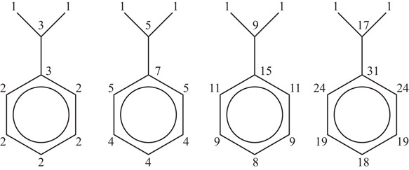
Figure 60.1Connectivity graph of cumin.
Initially, there are three distinct connectivity values. After the next iteration, there are four. Since the next two iterations both produce six distinct values, the end condition is triggered and the current (last iteration) is used as the final values.
While this algorithm works for almost all chemical structures, it can fail when the graph is highly regular producing oscillatory behavior. Morgan’s Algorithm has been adapted with approximation techniques to solve such problems [14]. As mentioned, many different versions of this algorithm have been produced. The variation from Chen et al. is O(mn2) where m is the number of starting points and n is the number of symmetry points [13].
60.2.3.2Nauty
One of the fastest algorithms for isomorphism testing and canonical naming is Nauty (No AUTomorphism, Yes?) [15]. It is based on a method of finding the automorphism group for a graph [16]. An automorphism is a mapping of a graph onto itself. A graph may have many such mappings, which are collectively referred to as the automorphism group.
Given a graph G(V, E), a partition of V is a set of disjoint subsets of V. The set of all partitions of V is denoted by Π(V). The divisions of a particular partition π are called its cells. A partition with one cell is called a unit partition and a partition in which each cell contains only one vertex is called a discrete partition. Given two partitions π1 and π2, π1 is finer than π2 (and π2 is coarser than π1) if every cell of π1 is a subset of some cell in π2. The unit partition is the coarsest partition and the discrete partition is the finest. The key to the algorithm is producing equitable partitions. A partition π is said to be equitable if, given a partition π of V into n cells (where a cell W is a set of vertices): π = W1, W2,…, Wn, π is equitable if for every cell Wi there exists a di such that every vertex in cell Wi is adjacent to exactly di vertices in cell Wi + 1. McKay [16] proves that every graph has a unique, coarsest equitable partition that is guaranteed to exist. The Nauty package implements a refinement process that takes any partition (usually a unit partition) as input and produces the unique equitable coarsest partition as output. The vertices are initially divided into cells by degree, sorted in increasing order. Each cell is then iteratively compared with subsequent cells by comparing the degrees in each cell. Whenever a discrepancy in degree is found, the cell is divided. If no discrepancies are found, the loop ends. Since a discrete partition cannot be further divided, it is also an end condition. Each cell in the partition is “colored” producing a unique name.
Given the graph in Figure 60.2, and the initial unit partition π = [01234], the initial refinement process would create the partition π = [34|01|2] which, for this simple example, is the coarsest equitable partition. Nodes 3 and 4 would be colored the same as would nodes 0 and 1.

Figure 60.2Graph for Nauty example.
The time complexity of Nauty was analyzed in Reference 17, where it is proven that the worst-case time complexity is exponential. In practice, when used on chemical graphs, Nauty appears to have a complexity that is linear.
60.2.3.3Signature-Based Canonization
This naming algorithm produces a molecular descriptor called a signature which is based on extended valence sequences [10].
The algorithm first constructs a graph, which is similar in form to a tree, for each atom in the molecule. The graph is not formally a tree since vertices representing atoms may appear more than once in the graph. The root of the “tree” is the atom being considered. The next level is composed of nodes representing all of the atoms connected to the root atom. The next level contains all of the atoms connected to atoms in the previous level. This process continues until all bonds in the molecule have been considered. As previously mentioned, it is possible that a node representing an atom could appear multiple times in the graph. In fact, when these repeated nodes occur at the same level, entire subtree structures are repeated. For this reason, the space requirements of the algorithm are minimized by pointing to repeated subtrees, thus forming a directed acyclic graph (DAG).
Each node in the tree is then initialized with an integer invariant that is derived from the represented atom’s type. Then, starting from the level furthest from the root, the nodes are sorted based on their invariants. The invariants of the nodes at the next level closer to the root are then recalculated based on their invariants and those of their neighbors. This process continues until the root is reached. The purpose of this procedure is the production of a unique ordering of the edges of the graph based on the node invariants.
The graph is then traversed in a depth-first manner, producing a signature for the atom. This signature contains enough information to completely rebuild the molecule. In fact, the molecule can be reconstructed from the signature produced for any of the atoms in the graph. The lexicographically largest signature of all of the atom signatures is used to represent the molecule. Since all signatures contain all of the needed information, the other signatures can be discarded. Pseudocode for Signature-based canonization follows.
1.For each atom in the molecule:
a.Create the signature tree with the current atom at the root
b.Assign initial integer invariant values
c.For each level of the signature tree, from the leaves to the root:
i.Sort the nodes at the current level, based on invariant values
ii.Recalculate the invariant values for the nodes on the next level using the values of the neighboring nodes
d.Produce a signature string for the atom based on a depth-first search for every node in the tree
e.Associate the signature string with the current atom
2.Choose the lexicographically largest signature string to represent the molecule
3.Discard all other signature strings.
The worst-case time complexity of the Signature algorithm on pathological inputs is exponential.
60.3Chemical Fingerprints and Similarity Search
Because of the difficulties associated with the graph isomorphism and subgraph isomorphism problems, molecules are encoded and stored in chemical databases as fingerprints. Chemical fingerprints are representations of 2D chemical structure and are used in chemical database substructure searching, similarity search, clustering, and classification. Several chemical fingerprinting schemes are described in the literature. One of these is the extended connectivity fingerprint (ECFP).
The ECFP is a circular fingerprint based on Morgan’s algorithm. ECFPs are not designed for substructure searches, but are instead used for similarity searches, clustering, and virtual screening. They are generated in three steps: (1) an initial assignment stage, where each atom is assigned an integer identifier; (2) an iterative updating stage in which each atom’s identifier is updated to include its neighbors; and (3) finally, a duplicate identifier removal stage. The ECFP set includes all of the identifiers generated in each iteration. For more details about ECFP and a comprehensive discussion of other fingerprint techniques, we refer the reader to Reference 18.
In the remainder of this chapter, we do not focus on a particular fingerprinting scheme, but on the underlying concept as illustrated in Figure 60.3.
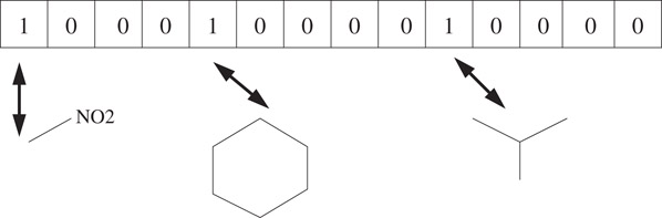
Figure 60.3Illustration of fingerprints: the fingerprint vector is a bit string with each element in the vector denoting a particular molecular substructure. Examples of substructure features used in the fingerprint include all possible labeled paths or labeled trees (circular substructures) up to a certain length. A bit is set to “1” if and only if the corresponding substructure is present in the molecule. In some versions, each element of the vector is a count of the number of occurrences of the particular substructure.
Given two sets a and b, the Tanimoto similarity S(a, b) between them is defined as
where |a| denotes the cardinality of set a. The cardinality of a set is given by the number of “1”s in the corresponding fingerprint. The Tanimoto similarity is well defined as long as at least one set is nonempty. Note that 0 ≤ S(a, b) ≤ 1, with S(a, b) = 0 when the intersection is empty and S(a, b) = 1 when the two sets are identical.
Tanimoto similarities are used to find all sets (represented by fingerprints) in a database that are similar to a query fingerprint as follows:
Given a database D of fingerprints and a query fingerprint q, return all fingerprints d∈D such that S(q, d) ≥ t, where t is a user-specified threshold.
Note that the time complexity of this operation is O(|D|f), where f denotes the time needed to compute the Tanimoto similarity between a pair of fingerprints, which is proportional to the length of the fingerprint vector.
An alternative formulation for similarity searches does not require the user to specify an arbitrary t, but instead returns the top C hits:
Given a database D of fingerprints and a query fingerprint q, return C fingerprints d∈D with the highest S(q, d) values.
This approach requires the computation of all Tanimoto similarities as before O(|D|f). A max-heap is used to keep track of the top C hits for an additional computation of O(|D| (log C). Given the large sizes of molecular databases, a linear search that compares a query fingerprint with each of the database fingerprints is unacceptably expensive. In the sections below, we describe several improvements to the linear search based on the use of innovative data structures.
One strategy [19] to improve search times is to use information about the cardinalities of both sets to reduce the number of database fingerprints against whom similarities are computed. For a given fixed |q| and |d|, S(q, d) is maximized when |q ∩ d| is maximized and |q ∪ d| is minimized. This occurs when q ⊆ d or d ⊆ q and results in the following bound:
Consider an example of a similarity search where the size of the query fingerprint |q| = 200 and the user-defined similarity threshold t = 0.8.
Case 1 |q| ≤ |d|: S(q, d) ≤ 200/|d|. Any fingerprints d ∈ D such that |d| > 250 result in S(q, d) ≤ 0.8 and can be immediately discarded without further analysis.
Case 2 |q| ≥ |d|: S(q, d) ≤ |d|/200. Any fingerprints d ∈ D such that |d| < 160 result in S(q, d) ≤ 0.8 and can also be immediately discarded.
Only d with 160 ≤ |d| ≤ 250 need to be evaluated further against query q. To exploit this observation, the database is preprocessed so that fingerprints are placed in bins indexed by size. Only bins corresponding to sizes in the range [|q|t,|q|/t] need to be searched.
This organization of fingerprints by cardinality can also be used in the top C hits formulation. We compute the bound for each bin and sort the bins in decreasing order of bound. The fingerprints are explored (i.e., their Tanimoto similarity against q is computed) in this order. Once again, a max-heap is used to store the top C hits. The search is terminated when the smallest similarity value in the heap is greater than the highest bound remaining.
Fingerprints can be very long (215 − 220 bits) and sparse. Recall that the computation time for similarity and top-C searches includes a factor f corresponding to fingerprint size. Compressing fingerprints not only reduces the size of the database but also improves computation time. Long fingerprints may be compressed by a factor of k by folding them using a simple modulo operation.
Compressed fingerprints can now be used instead of the original fingerprints for similarity searches as described earlier. This introduces an error that results in a systematic overestimate of Tanimoto similarity. (A given bit location in a pair of compressed fingerprints could both be 1 even though none of the corresponding k pairs of bits in the original fingerprints were both “1”s.) Molecules that would not meet the similarity threshold using the original fingerprints might meet them using compressed fingerprints. This overestimate results in a reduction in the quality of the similarity search. A mathematical correction of this overestimate is derived in Reference 20.
The folding scheme described above is lossy because it is not possible to recover the original fingerprint from the compressed fingerprint. An alternative lossless approach for reducing fingerprint size exploits the sparsity of fingerprints by storing the indices of “1” bits. In the example, (1 0 0 0 1 1 0 0 0 0 0 0 1 0 1) can be represented by (1 5 6 13 15). Another approach is to store the lengths of 0 runs: (0 3 6 1) in our example. These reduced vectors can be compressed optimally using Golomb-Rice or Elias Codes based on statistical assumptions [21].
60.3.4Hashing Approaches for Improved Searches
Additional improvements over the bounds presented in Section 60.3.2 can be obtained by associating with each fingerprint a short integer signature vector of length M. When M = 1, the integer is simply the number of “1”s in the fingerprint, making the improvement of Section 60.3.2 a special case of this approach. The case when M = 5 is illustrated by a simple modification to the example in Figure 60.4: instead of taking the OR of corresponding bits, we add their values giving the vector (2 0 1 0 2).
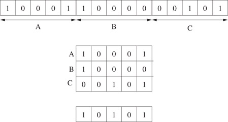
Figure 60.4Illustration of folding: a long fingerprint consisting of 15 bits (1 0 0 0 1 1 0 0 0 0 0 0 1 0 1) is folded by a factor of 3 to give a fingerprint (1 0 1 0 1) of length 5. The original fingerprint is interpreted as having been subdivided into three segments of length 5 each. Bit j in the compressed fingerprint is the logical OR of bits j in the three segments.
In our explanation, we focus on the case where M = 2. The two integers in this case may be obtained by separately counting the number of “1”s in the first half and the second half, respectively. For fingerprint q, the two counts are denoted by q1 and q2, respectively.
We can now compute a bound on S(q, d) as follows:
From, this we get . There are now four cases, depending on the outcome of the min operations:
1.
2.
3.
4..
The first two cases give us |q|t ≤ |d| ≤ |q|/t, the inequalities corresponding to M = 1, identical to those obtained in Section 60.3.2. For a fixed value of |d|, cases 3 and 4 give us − q2 + t(|q| + |d|)/(t + 1) < d1 < |d| + q1 − t(|q| + |d|)/(1 + t). Consider an example with |q| = 200 and t = 0.8 as before. Recall that this already reduces the search to values of |d| in [160, 250]. Suppose q1 = 125 and q2 = 75. Suppose also that we are considering database fingerprints with |d| = 200. Substituting, this gives 102 < d1 < 147. This allows us to further eliminate fingerprints in the |d| = 200 bin that do not meet this criteria. This computation is facilitated by a secondary sorting within each bin on d1. Recall that bins are already ordered by |d|.
60.3.5Triangle Inequality and Improvements
Recall that Tanimoto similarity is guaranteed to be in the range [0, 1] with a high value denoting a high similarity and vice versa. We can also define Tanimoto distance D(a, b) = 1 − S(a, b). The Tanimoto distance is a distance metric and satisfies the triangle inequality; that is, given three fingerprints a, b, and c: |D(b, a) − D(a, c)| ≤ D(b, c) ≤ D(b, a) + D(a, c). This inequality can be used to prune searches as follows: suppose D(a, b) is small (say 0.1) and D(a, c) is large (say 0.9). We have 0.8 ≤ D(b, c) ≤ 1.0, which implies that 0 ≤ S(b, c) ≤ 0.2. For t > 0.2, we are able to avoid computing S(b, c). Notice that this computation does not utilize information about the precise bits that are common between a and c or a and b to compute a bound between b and c. A more sophisticated analysis that considers this information gives an intersection bound that is tighter than the distance bound that results in more efficient searches [22].
Another strategy [23] for improving similarity searches is to augment the original fingerprint with a signature: a folded fingerprint based on the XOR operator unlike the example in Figure 60.4 which uses the OR operator. The XOR-based signature on the example is (0, 0, 1, 0, 0). The signature is used to prune the search space as described below.
First, note that the union and intersection used in the computation of Tanimoto’s similarity can be expressed in terms of the XOR (⊕) operator as follows. In set-theoretic terms, |a ⊕ b| = |a − b| + |b − a|.
Let the XOR-folded fingerprints of a and b be α and β, respectively. We then have |a ⊕ b| ≥ |α ⊕ β|, which gives.
resulting in
If the quantity in the RHS is less than the similarity threshold t, we can discontinue the computation of S(a, b). The XOR filter will sometimes result in better bounds than BitBound and can be used in addition to it.
Consider a database of |D| molecules represented as f-bit binary fingerprints, with each bit i, 1 ≤ i ≤ f, corresponding to the presence/absence of a feature. In an inverted index, a list of molecules is maintained for each of the f features. List i consists of all molecules whose ith bit is set to 1. Consider the fingerprint corresponding to a query molecule q. In order to compute its Tanimoto similarity with each fingerprint in the database, we only need to traverse the lists corresponding to features present in q. We maintain a counter for each molecule in D that is initialized to 0. When a molecule is encountered in one of the relevant lists, its counter is incremented. The final value of the counter for each molecule represents the size of its intersection with the query molecule, the numerator of the Tanimoto similarity formula.
Nasr et al. note that the similarity threshold problem can be reduced to the T occurrence problem in information retrieval (i.e., finding all fingerprints with an intersection of size at least T with the query), for which efficient solutions based on the inverted index exist. We have
which gives
The invertex index-based DivideSkip solution [24] to the T-occurrence problem is presented and applied in Reference 23.
A set of LINGOs [25] is defined as all substrings of length q in the modified SMILES string for a molecule. A simplified SMILES string S = c0ccccc0L for q = 4 gives the multiset {c0cc, 0ccc, cccc, cccc, ccc0, cc0L}. The similarity between two molecules represented by their SMILES strings can be computed as the Tanimoto similarity between their LINGO multisets (LINGOsim). The LINGOsim computation is performed by representing the LINGOs of the query by a trie/finite state machine to improve the efficiency of the computation [26]. An alternative solution stores the database of molecules (with each molecule represented by a LINGO multiset) as an inverted index [27].
60.3.9Trie-Based Approaches for Storing Fingerprints
A database of binary fingerprints can be stored in a binary tree. Starting with the root, the complete set of fingerprints is recursively split into two sets corresponding to its left and right subtrees. Each fingerprint is assigned to one of the two sets depending on the value of its first (leftmost) bit. If the value is 0 (1), it is assigned to the left (right) subtree. At level i of the tree, bit i of the fingerprint is used to determine the assignment of the fingerprint to the appropriate subtree. For an exact search for a fingerprint, the algorithm starts at the root and follows left or right pointers that spell out the fingerprint in time proportional to f.
For a threshold similarity search, a naive solution visits all of the leaves of the trie and computes the Tanimoto similarity. This search can be pruned be employing the Tanimoto lookahead condition [28] described later. Let
1.B(n, d) denote the partial bit string spelled by the path from the root to node n at depth d.
2.Q(d) denote the partial bit string formed from the first d bits of the query fingerprint.
3.QL(d) denote the number of “1”s in the query bit string after position d.
The Running Union Count and Running Intersection Counts are defined respectively as RUC(n, d) = |B(n, d) ∪ Q(d)| and RIC(n, d) = |B(n, d) ∩ Q(d)|. The maximum value of the Tanimoto similarity between query q and any molecule that is reached by traversing the bit tree through node n is given by
The search can be terminated at node n if this value computed at node n is less than the threshold t.
A more efficient organization of the tree splits the fingerprints into two sets using a bit of maximal entropy (i.e., one that yields two subsets as much as possible of equal size) rather than picking the next bit in left-to-right order. This is the Singlebit tree described in Reference 29. The equation for Smax above applies to the modified tree, but requires that each tree node keep track of the bit used at that node as well as the bits used by its ancestors to split the fingerprint set.
60.3.10Multibit and Union Tree
The Singlebit tree was found to be inefficient in experiments [29] because a relatively small tree depth was found to be enough to partition the fingerprints. This meant that the algorithm is only aware of a small fraction of bits, resulting in bounds that do not prune a large number of fingerprints.
The Multibit tree addresses this shortcoming by recording in each node the list of bits that have constant value 0 or 1 in all of the fingerprints stored in the node’s subtree. For example, consider a node whose subtree contains two fingerprints: 10, 101, and 10110. The node would store the three common bits as (1,1) (2,0) (3,1) where the first element denotes the position of the bit and the second is the common value. Using this information results in tighter bounds and greater pruning [29,30].
An alternative strategy (UnionBit Tree) has a node store the union of the fingerprint vectors in its leaves. In the example above, the node would store 10111. A query fingerprint’s intersection with the union vector has cardinality guaranteed to be greater than or equal to that of any of the individual fingerprints. The UnionBit tree uses less CPU time and memory relative to the MultiBit treei [31].
60.3.11Combining Hashing and Trees
The BitBound algorithm (described in Section 60.3.2) organizes fingerprints by placing each fingerprint in a bin corresponding to its cardinality, the number of 1s in that fingerprint; that is, all fingerprints with 15 1s are placed in bin 15. The bins are sorted by cardinality; the BitBound algorithm searches bins in a specified range as described earlier. Improved solutions are obtained by storing the fingerprints in each bin using a multibit tree [30].
1.N. Brown, Chemoinformatics—An introduction for computer scientists, ACM Computing Surveys, vol. 41, no. 2, pp. 8:1–8:38, February 2009.
2.J. K. Wegner, A. Sterling, R. Guha, A. Bender, J.-L. Faulon, J. Hastings, N. O’Boyle, J. Overington, H. Van Vlijmen, and E. Willighagen, Cheminformatics, Communications of the ACM, vol. 55, no. 11, pp. 65–75, November 2012.
3.J.-L. Faulon, and A. Bender, Handbook of Cheminformatics Algorithms, Boca Raton, FL: CRC Press, 2010.
4.D. J. Wild, Introducing Cheminformatics: An Intensive Self-Study Guide, McGraw-Hill Open-publishing, 2013.
5.J. E. Hopcroft and J. K. Wong, Linear time algorithm for isomorphism of planar graphs (preliminary report), in STOC’74: Proceedings of the Sixth Annual ACM Symposium on Theory of Computing. New York, NY: ACM Press, 1974, pp. 172–184.
6.M. R. Garey and D. S. Johnson, Computers and Intractability; A Guide to the Theory of NP-Completeness, New York, NY: W. H. Freeman & Co., 1990.
7.A. Aho, J. Hopcroft, and J. Ullman, The Design and Analysis of Computer Algorithms, Reading, MA: Addison-Wesley, 1974.
8.E. Luks, Isomorphism of graphs of bounded valence can be tested in polynomial time, Journal of Computer and System Sciences, vol. 25, no. 1, pp. 42–65, August 1982.
9.C. M. Hoffmann, Group-Theoretic Algorithms and Graph Isomorphism, Springer-Verlag GmbH and Co. KG: Berlin/Heidelberg, December 1982.
10.J.-L. Faulon, M. J. Collins, and R. D. Carr, The signature molecular descriptor. 4. Canonizing molecules using extended valence sequences, Journal of Chemical Information and Modeling, vol. 44, no. 2, pp. 427–436, 2004. [Online]. Available: http://dx.doi.org/10.1021/ci0341823
11.T. M. Kouri, D. Pascua, and D. P. Mehta, Random models and analyses for chemical graphs, International Journal of Foundations of Computer Science, vol. 26, no. 2, pp. 269–291, 2015.
12.H. L. Morgan, The generation of a unique machine description for chemical structures—A technique developed at chemical abstracts service, Journal of Chemical Documentation, vol. 5, no. 2, pp. 107–113, 1965.
13.W. Chen, J. Huang, and M. K. Gilson, Identification of symmetries in molecules and complexes, Journal of Chemical Information and Modeling, vol. 44, no. 4, pp. 1301–1313, 2004.
14.T. Cieplak and J. Wisniewski, A new effective algorithm for the unambiguous identification of the stereochemical characteristics of compounds during their registration in databases, Molecules, vol. 6, 915–926, 2001.
15.B. McKay, No automorphisms, yes?” http://cs.anu.edu.au/bdm/nauty/, 2004.
16.B. McKay, Practical graph isomorphism, Congressus Numerantium, vol. 30, 45–87, 1981.
17.T. Miyazaki, The complexity of McKay’s canonical labeling algorithm, Groups and Computation II, DIMACS Series in Discrete Mathematics and Theoretical Computer Science, vol. 28, 239–256, 1997.
18.D. Rogers and M. Hahn, Extended-connectivity fingerprints, Journal of Chemical Information and Modeling, vol. 50, no. 5, pp. 742–754, 2010.
19.S. J. Swamidass and P. Baldi, Bounds and algorithms for fast exact searches of chemical fingerprints in linear and sublinear time, Journal of Chemical Information and Modeling, vol. 47, no. 2, pp. 302–317, 2007.
20.S. J. Swamidass and P. Baldi, Mathematical correction for fingerprint similarity measures to improve chemical retrieval, Journal of Chemical Information and Modeling, vol. 47, no. 3, pp. 952–964, 2007.
21.P. Baldi, R. W. Benz, D. S. Hirschberg, and S. J. Swamidass, Lossless compression of chemical fingerprints using integer entropy codes improves storage and retrieval, Journal of Chemical Information and Modeling, vol. 47, no. 6, pp. 2098–2109, 2007.
22.P. Baldi and D. S. Hirschberg, An intersection inequality sharper than the Tanimoto triangle inequality for efficiently searching large databases, Journal of Chemical Information and Modeling, vol. 49, no. 8, pp. 1866–1870, 2009.
23.P. Baldi, D. S. Hirschberg, and R. J. Nasr, Speeding up chemical database searches using a proximity filter based on the logical exclusive or, Journal of Chemical Information and Modeling, vol. 48, no. 7, pp. 1367–1378, 2008.
24.C. Li, J. Lu, and Y. Lu, Efficient merging and filtering algorithms for approximate string searches,’ in Proceedings of the 2008 IEEE 24th International Conference on Data Engineering, series ICDE’08. Washington, DC: IEEE Computer Society, 2008, pp. 257–266.
25.D. Vidal, M. Thormann, and M. Pons, Lingo, an efficient holographic text based method to calculate biophysical properties and intermolecular similarities, Journal of Chemical Information and Modeling, vol. 45, no. 2, pp. 386–393, 2005.
26.J. A. Grant, J. A. Haigh, B. T. Pickup, A. Nicholls, and R. A. Sayle, Lingos, finite state machines, and fast similarity searching, Journal of Chemical Information and Modeling, vol. 46, no. 5, pp. 1912–1918, 2006.
27.T. G. Kristensen, J. Nielsen, and C. N. S. Pedersen, Using inverted indices for accelerating lingo calculations, Journal of Chemical Information and Modeling, vol. 51, no. 3, pp. 597–600, 2011.
28.A. Smellie, Compressed binary bit trees: A new data structure for accelerating database searching, Journal of Chemical Information and Modeling, vol. 49, no. 2, pp. 257–262, 2009.
29.T. Kristensen, J. Nielsen, and C. Pedersen, A tree based method for the rapid screening of chemical fingerprints, in Algorithms in Bioinformatics, series Lecture Notes in Computer Science, S. Salzberg and T. Warnow, Eds. Springer, Berlin/Heidelberg, 2009, vol. 5724, pp. 194–205.
30.R. Nasr, T. Kristensen, and P. Baldi, Tree and hashing data structures to speed up chemical searches: Analysis and experiments, Molecular Informatics, vol. 30, no. 9, pp. 791–800, 2011.
31.S. Saeedipour, D. Tai, and J. Fang, Chemcom: A software program for searching and comparing chemical libraries, Journal of Chemical Information and Modeling, vol. 55, no. 7, pp. 1292–1296, 2015.