Example with a Nonsignificant Interaction
To illustrate how a two-way ANOVA is performed, let’s modify the earlier study that examined the effect of rewards on commitment in romantic relationships. In Chapter 9, “One-Way ANOVA with One Between-Subjects Factor,” only one independent variable was manipulated, and this variable was called “type of rewards.” In this chapter, however, there are two independent variables: independent variable A will be “type of rewards” while independent variable B will be “type of costs.”
In the study presented in Chapter 9, participants read descriptions of a fictitious “partner 10” and rated how committed they would be to a relationship with that person. One independent variable (called “type of rewards”) was manipulated, and this variable consisted of three experimental conditions. Participants were assigned to either the low-, mixed-, or the high-reward conditions. This variable was manipulated by varying the description of partner 10 which was provided to participants:
Participants in the low-reward condition were told to assume that this partner “...does not enjoy the same recreational activities that you enjoy, and is not very good looking.”
Participants in the mixed-reward condition were told to assume that “...sometimes this person seems to enjoy the same recreational activities that you enjoy, and sometimes s/he does not. Sometimes partner 10 seems to be very good looking, and sometimes s/he does not.”
Participants in the high-reward condition were told that this partner “...enjoys the same recreational activities that you enjoy, and is very good looking.”
These same manipulations will be used in the present study. In a sample of 30 participants, one-third will be assigned to a low-reward condition, one-third to a mixed-reward condition, and one-third to a high-reward condition. This “type of reward” factor serves as independent variable A.
In this study, however, you also manipulate a second predictor variable (independent variable B) at the same time. The second independent variable will be called “type of costs” and it will consist of two experimental conditions. Half the participants (the “low-cost” group) will be told to assume that they are in a relationship that does not create significant personal hardships. Specifically, when they read the description of partner 10, it will state that “Partner 10 lives in the same neighborhood as you so it is easy to see him/her as often as you like.” The other half of the participants (the “high-cost” group) will be told to imagine that they are in a relationship that does create significant personal hardships. When they read the description of partner 10, it will state that “Partner 10 lives in a distant city, so it is difficult and expensive to visit with him/her.”
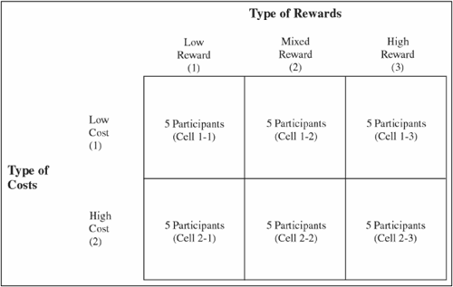
Your study now has two independent variables. Independent variable A is type of rewards and it has three levels (or conditions); independent variable B is type of costs and it has two levels. The factorial design used in the study is illustrated in Figure 10.7.
This 2 × 3 matrix shows that there are two independent variables. One independent variable has two levels, and the other has three levels. There are a total of 30 participants who are divided into 6 cells or subgroups. Each cell contains five participants. Each horizontal row in the figure (running from left to right) represents a different level of the type of costs independent variable. There are 15 participants in the low-cost condition and 15 in the high-cost condition. Each vertical column in the figure (running from top to bottom) represents a different level of the type of rewards independent variable. There are 10 participants in the low-reward condition, 10 in the mixed-reward condition, and 10 in the high-reward condition.
It is strongly advised that you prepare a similar figure whenever you conduct a factorial study, as this will make it easier to enter your data and reduce the likelihood of input errors. Notice that the cell designator (the cell number, such as “1-1,” “2-3,” etc.) indicates which experimental condition to which a given participant was assigned under each of the two independent variables. The first number in the designator indicates which level under type of costs and the second number indicates level of rewards. For example, the designator “1-1” for cell 1-1 indicates that the participant was in condition 1 (the low-cost condition) under type of costs and in condition 1 (the low-reward condition) under type of rewards. This means that all five participants in this subgroup read that partner 10 lives in the same town as the participant (low-cost) but is not very good-looking (low-reward).
On the other hand, the designator “2-3” for cell 2-3 indicates that the participant was in condition 2 (the high-cost condition) under type of costs and was in condition 3 (the high-reward condition) under type of rewards. This means that all five participants in this subgroup read that partner 10 lives in a distant city (high-cost), but is very good-looking (high-reward). Similar reasoning applies in the interpretation of the designators for the remaining four cells in the figure.
When working with these cell designators, remember that the number for the row precedes and the number for the column. This means that the cell at the intersection of row 2 and column 1 is identified with the designator 2-1, not 1-2.
Writing the SAS Program
Creating the SAS Dataset
There were two predictor variables in this study (type of rewards and type of costs) and one criterion variable (commitment). This means that each participant has a score for three variables. First, with the variable REWGRP, you indicate which experimental condition this participant experienced under the type of rewards independent variable. Each participant is given a score of 1, 2, or 3 depending on the condition to which s/he is assigned. Second, with the variable COSTGRP, you indicate which condition the participants are assigned under the type of costs independent variable. Each participant is given a score of either 1 or 2 depending on the condition to which s/he is assigned. Finally, with the variable COMMIT, you will record participants’ rated commitment to the relationship with partner 10. That is, you simply enter the number that is the sum of responses to the four questionnaire items that measure commitment to partner 10.
The data are entered so that there is one line of data for each participant. Assume that you enter your data using the following format:
| Line | Column | Variable Name | Explanation |
|---|---|---|---|
| 1 | 1 | COSTGRP | Codes group membership, so that
1 = low-cost condition, and 2 = high-cost condition |
| 2 | blank | ||
| 3 | REWGRP | Codes group membership, so that
1 = low-reward condition, 2 = mixed-reward condition, and 3 = high-reward condition | |
| 4 | blank | ||
| 5-6 | COMMIT | Commitment ratings obtained when participants rated partner 10 |
Remember that there are actually 30 participants in your study. However, to save space, assume for the moment that there are only 12 participants: two participants in cell 1-1; two participants in cell 1-2; and so forth. Here is what the dataset might look like if it were keyed according to the preceding format:
 1          1 1 08
 2          1 1 07
 3          1 2 13
 4          1 2 17
 5          1 3 36
 6          1 3 31
 7          2 1 09
 8          2 1 10
 9          2 2 15
10          2 2 18
11          2 3 35
12          2 3 29
Remember that the numbers on the far left are simply line numbers for reference; they are not actually a part of the dataset. In the dataset itself, the first vertical column of numbers (in column 1) codes the COSTGRP variable. Notice that participants who appear in lines 1 to 6 of the preceding dataset have a score of “1” for COSTGRP (indicating that they are in the low-cost condition.) In contrast, the participants on lines 7 to 12 of the preceding dataset have a score of “2” for COSTGRP indicating that they are in the high-cost condition.
The second column of numbers (in column 3) codes REWGRP. For example, the two participants from lines 1 to 2 of the preceding program have scores of “1” for REWGRP (indicating that they are in the low-reward condition), the two participants from lines 3 to 4 have scores of “2” on REWGRP (indicating that they are in the mixed-reward condition), and the two participants from lines 5 to 6 have scores of “3” for REWGRP (indicating that they are in the high-reward condition).
Finally, the last grouping in the dataset (columns 5 to 6) codes COMMIT (i.e., commitment scores from the participants). Assume that, with this variable, scores could range from 4 to 36 with higher scores representing higher levels of commitment to partner 10. You can see that the participant from line 1 had a score of “08” for COMMIT, the participant from line 2 had a score of “07,” and so forth.
This approach to entering data for a two-way ANOVA is particularly useful because it provides a quick way to determine the cell (from the factorial design matrix) in which a given participant can be found. For example, the first two columns of data for the participant from line 1 provide the values “1” and “1” (indicating that this participant is in cell 1-1). Similarly, the first two columns for the participant from line 5 are “1” and “3” (indicating that this participant is in cell 1-3). The data in the preceding dataset are sorted so that participants in the same cell are grouped together; note that your data do not actually have to be sorted this way to be analyzed with PROC GLM.
Testing for Significant Effects with PROC GLM
Here is the general form for the PROC GLM step needed to perform a two-way ANOVA and follow it up with Tukey’s HSD test. Enter your file name where filename appears.
PROC GLM DATA= filename;
   CLASS  predictorA predictorB;
   MODEL  criterion-variable = predictorA predictorB
          predictorA*predictorB;
   MEANS  predictorA predictorB / TUKEY;
   MEANS  predictorA predictorB predictorA*predictorB;
RUN;
This is the entire program, including the DATA step, needed to analyze some fictitious data from the preceding study:
 1             DATA D1;
 2                INPUT   #1  @1 COSTGRP 1.
 3                            @3 REWGRP  1.
 4                            @5 COMMIT  2.  ;
 5             DATALINES;
 6             1 1 08
 7             1 1 13
 8             1 1 07
 9             1 1 14
10             1 1 07
11             1 2 19
12             1 2 17
13             1 2 20
14             1 2 25
15             1 2 16
16             1 3 31
17             1 3 24
18             1 3 37
19             1 3 30
20             1 3 32
21             2 1 09
22             2 1 14
23             2 1 05
24             2 1 14
25             2 1 16
26             2 2 22
27             2 2 18
28             2 2 20
29             2 2 19
30             2 2 21
31             2 3 24
32             2 3 33
33             2 3 24
34             2 3 26
35             2 3 31
36             ;
37             RUN;
38
39             PROC GLM DATA=D1;
40                CLASS REWGRP COSTGRP;
41                MODEL COMMIT = REWGRP COSTGRP REWGRP*COSTGRP;
42                MEANS REWGRP COSTGRP / TUKEY;
43                MEANS REWGRP COSTGRP REWGRP*COSTGRP;
44             RUN;
Notes Regarding the SAS Program
The GLM procedure is requested on line 39. In line 40, both REWGRP and COSTGRP are listed as classification variables.
The MODEL statement on line 41 specifies COMMIT as the criterion variable and lists three predictor terms: REWGRP; COSTGRP; and REWGRP*COSTGRP. The last term (REWGRP*COSTGRP) is the interaction term in the model. You create this interaction term by typing the names of your two predictor variables, connected by an asterisk (and no blank spaces).
The program includes two MEANS statements. The MEANS statement on line 42 requests that the Tukey multiple comparison procedure be used with predictor variables REWGRP and COSTGRP. (Do not list the interaction term in this MEANS statement.) The MEANS statement on line 43 requests that means be printed for all levels of REWGRP and COSTGRP. You should include the interaction term in this MEANS statement to obtain means for each of the six cells from the study’s factorial design.
Steps in Interpreting the Output
With LINESIZE=80 and PAGESIZE=60 in the OPTIONS statement (first line), the preceding program would produce five pages of output. The information that appears on each page is summarized here:
Page 1 provides class level information and the number of observations in the dataset.
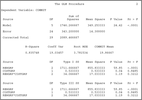
Page 2 provides the ANOVA summary table from the GLM procedure.
Page 3 provides the results of the Tukey multiple comparison procedure for the REWGRP independent variable.
Page 4 provides the results of the Tukey multiple comparison procedure for the COSTGRP independent variable.
Page 5 provides three tables that summarize the means observed for the various groups that constitute the study:
The first table provides the means observed at each level of REWGRP.
The second table provides the means observed at each level of COSTGRP.
The third table provides the means observed for each of the six cells in the study’s factorial design.
The results produced by the preceding program are reproduced here as Output 10.1.
Output 10.1. Results of Two-Way ANOVA Performed on Investment Model Data, Nonsignificant Interaction
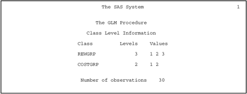

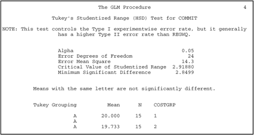
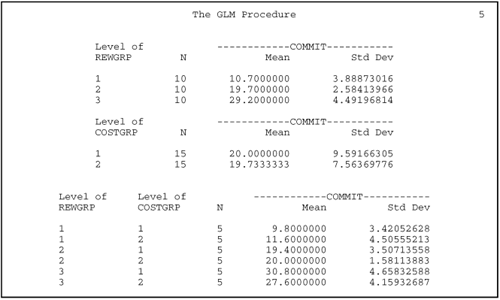
The fictitious dataset analyzed in this section was designed so that the interaction term would be nonsignificant. When the interaction is nonsignificant, interpreting the results of a two-factor ANOVA is very similar to interpreting the results of a one-factor ANOVA. Therefore, many of the instructions provided in the chapter on one-way ANOVA (Chapter 9) will not be repeated here (“making sure page 1 looks right,” etc.). Instead, this section focuses on some issues that are specific to a two-factor ANOVA. The steps to follow in interpreting the output are discussed next.
1. Determine Whether the Interaction Term Is Statistically Significant
Two-factor ANOVA allows you to test for three types of effects: (a) the main effect of predictor A (type of rewards, in this case); (b) the main effect of predictor B (type of costs); and (c) the interaction of predictors A and B. Remember that you may interpret a main effect only if the interaction is nonsignificant. One of your first steps must be to determine whether the interaction is significant. You can do this by looking at the analysis of variance results, which appears on page 2 of Output 10.1. (As before, look in the section that provides the “Type III SS.”) Toward the bottom left of page 2, you see the heading “Source,” as you did with the one-way ANOVA. In this case, however, you see three entries under “Source,” indicating that there are three sources of variation in your data: (a) REWGRP; (b) COSTGRP; and (c) REWGRP*COSTGRP. The last entry, REWGRP*COSTGRP, is the interaction term in which you are interested. If this interaction is significant, it suggests that the relationship between one predictor and the criterion variable is different at different levels of the second predictor. In the present case, the interaction is associated with 2 degrees of freedom, a value of approximately 34.07 for the Type III sum of squares, a mean square of 17.03, an F value of 1.19, and a corresponding p value of .32. Remember that you generally view a result as being statistically significant only if the p value is less than .05. Since this p value of .32 is larger than .05, you conclude that there is no interaction between the two independent variables. You are therefore free to proceed with your review of the two main effects.
2. Determine If Either of the Main Effects Is Statistically Significant
A two-way ANOVA allows you to test two null hypotheses concerning main effects. The null hypothesis for the type of rewards predictor can be stated as follows:
In the population, there is no difference between the high-reward group, the mixed reward group, and the low-reward group with respect to scores on the commitment variable.
The F statistic to test this null hypothesis can again be found toward the bottom of page 2 in Output 10.1. To the right of the heading “REWGRP,” you can see that this effect is associated with 2 degrees of freedom, a value of approximately 1711.67 for the Type III sum of squares (rounded to two decimal places), a mean square of 855.83, an F value of 59.85, and a p value less than 0.01. With such a small p value, you can reject the null hypothesis of no main effect for type of rewards. Later, you will review the results of the Tukey test to see which pairs of groups (low-reward, high-reward, etc.) significantly differ.
The null hypothesis for the type of costs independent variable can be stated in a similar fashion:
In the population, there is no difference between the high-cost group and the low-cost group with respect to scores on the commitment variable.
The appropriate F statistic is once again found toward the bottom of page 2. To the right of “COSTGRP,” you see that this effect is associated with 1 degree of freedom, a value of approximately 0.53 for the Type III sum of squares, a mean square of 0.53, an F value of 0.04, and a p value of .85. This p value is greater than .05; therefore, you cannot reject the null hypothesis and, instead, conclude that there is not a significant main effect for type of costs.
3. Prepare Your Own Version of the ANOVA Summary Table
Use the information from page 2 of Output 10.1 to prepare the ANOVA summary table for the analysis. That table is reproduced here as Table 10.1.
| Source | df | SS | MS | F | R2 |
|---|---|---|---|---|---|
| Type of rewards (A) | 2 | 1711.67 | 855.83 | 59.85[*] | .82 |
| Type of costs (B) | 1 | 0.53 | 0.53 | 0.04 | .00 |
| A × B Interaction | 2 | 34.07 | 17.03 | 1.19 | .02 |
| Within groups | 24 | 343.20 | 14.30 | ||
| Total | 29 | 2089.47 | |||
| Note: N = 30. |
[*] p < .01
On page 2 of Output 10.1, to the right of “REWGRP*COSTGRP,” you will find information concerning the study’s interaction term. In your own ANOVA summary table (such as Table 10.1), this will appear on the line headed “A × B Interaction.” As was the case with one-way ANOVA, look to the right of the word “Error” to find the information needed for the “Within Groups” line of your table, and look to the right of “Corrected Total” to find the information needed for the “Total” line of your table.
In the preceding chapter, you learned that R2 is a measure of the strength of the relationship between a predictor variable and a criterion variable. In a one-way ANOVA, R2 tells you what percent of variance in the criterion is accounted for by the study’s predictor variable. In a two-way ANOVA, R2 indicates what percent of variance is accounted for by each predictor variable, as well as by their interaction term.
As is the case in Chapter 9, you will have to perform a few hand calculations to compute these R2 values. To calculate R2 for a given effect, divide the Type III sum of squares associated with that effect by the corrected total sum of squares. For example, to calculate the R2 value for the type of rewards main effect, you would take the appropriate terms from page 2 of Output 10.1 (or Table 10.1) and substitute them in the formula for R2, as is done here:
![]()
4. Review the Sample Means and Results of the Multiple Comparison Procedures
If a given main effect is statistically significant, you can review the Tukey test results for that main effect. Do this in the same way you would if this had been a one-way ANOVA. The results of the Tukey test for the present analysis are presented on pages 3 and 4 of Output 10.1. In this analysis, the type of rewards effect was significant, and the Tukey results on page 3 of Output 10.1 show that all three experimental groups are significantly different from each other, with the high-reward group showing the highest commitment scores, the mixed-reward group the next highest, and the low-reward group the lowest. (Chapter 9 describes how to interpret the Tukey test.)
The results of the Tukey test for the type of costs main effect appear on page 4 of Output 10.1. However, the type of costs main effect is not statistically significant; so, the Tukey results for that effect will not be interpreted. Technically, it would not really have been necessary to review the results of this multiple comparison procedure even if the type of costs main effect had been significant. This is because COSTGRP consists of only two groups, which means that you would not need a multiple comparison procedure to determine which “pairs” of groups were significantly different.
5. Summarize the Results of Your Analyses
In performing a two-way ANOVA, you should use the same statistical interpretation format as was used with one-way ANOVA:
Statement of the problem
Nature of the variables
Statistical test
Null hypothesis (H0)
Alternative hypothesis (H1)
Obtained statistic
Obtained probability (p) value
Conclusion regarding the null hypothesis
Magnitude of treatment effect
ANOVA summary table
Figure representing the results
However, with two-way ANOVA, it would be possible to perform this summary three times, since it is possible to test three null hypotheses in this study:
The hypothesis of no interaction (which would be stated: “In the population, there is no interaction between type of rewards and type of costs in the prediction of commitment scores.”)
The hypothesis of no main effect for predictor A (type of rewards).
The hypothesis of no main effect for predictor B (type of costs).
Because you should be fairly familiar with this format at this time, it is not completed again at this point.
Formal Description of Results for a Paper
Below is one approach that could be used to summarize the results of the preceding analysis in a scholarly paper:
Results were analyzed using two-way ANOVA, with two between-subjects factors. This analysis revealed a significant main effect for type of rewards, F(2, 24) = 59.85; p < .01 and large treatment effect, R2 = .82. The sample means are displayed in Figure 1. Tukey's HSD test indicated that participants in the high-reward condition scored significantly higher on commitment than did those in the mixed-reward condition, who, in turn, scored significantly higher than participants in the low-reward condition (p < .05). The main effect for type of costs proved to be nonsignificant, F(1, 24) = 0.04; ns. The interaction between type of rewards and type of costs also proved to be nonsignificant F(2, 24) = 1.19; ns.
