Most of this book is about the design of alpha factors using ML models. ML is about optimizing some predictive objective, and in this section, we will introduce the key metrics used to measure the performance of an alpha factor. We will define alpha as the average return in excess of a benchmark.

This leads to the information ratio (IR) that measures the average excess return per unit of risk taken by dividing alpha by the tracking risk. When the benchmark is the risk-free rate, the IR corresponds to the well-known Sharpe ratio, and we will highlight crucial statistical measurement issues that arise in the typical case when returns are not normally distributed. We will also explain the fundamental law of active management that breaks the IR down into a combination of forecasting skill and a strategy's ability to effectively leverage the forecasting skills.

The goal of alpha factors is the accurate directional prediction of future returns. Hence, a natural performance measure is the correlation between an alpha factor's predictions and the forward returns of the target assets. 

It is better to use the non-parametric Spearman rank correlation coefficient that measures how well the relationship between two variables can be described using a monotonic function, as opposed to the Pearson correlation that measures the strength of a linear relationship. 

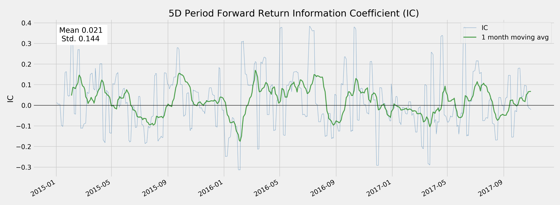
We can obtain the information coefficient using alphalens, which relies on scipy.stats.spearmanr under the hood (see the repo for an example on how to use scipy directly to obtain p-values). The factor_information_coefficient function computes the period-wise correlation and plot_ic_ts creates a time-series plot with one-month moving average:

from alphalens.performance import factor_information_coefficient
from alphalens.plotting import plot_ic_ts
ic = factor_information_coefficient(alphalens_data)
plot_ic_ts(ic[['5D']])

This time series plot shows extended periods with significantly positive moving-average IC. An IC of 0.05 or even 0.1 allows for significant outperformance if there are sufficient opportunities to apply this forecasting skill, as the fundamental law of active management will illustrate:

A plot of the annual mean IC highlights how the factor's performance was historically uneven:

ic = factor_information_coefficient(alphalens_data)
ic_by_year = ic.resample('A').mean()
ic_by_year.index = ic_by_year.index.year
ic_by_year.plot.bar(figsize=(14, 6))

This produces the following chart:

An information coefficient below 0.05 as in this case, is low but significant and can produce positive residual returns relative to a benchmark as we will see in the next section. The create_summary_tear_sheet(alphalens_data) creates IC summary statistics, where the risk-adjusted IC results from dividing the mean IC by the standard deviation of the IC, which is also subjected to a two-sided t-test with the null hypothesis IC = 0 using scipy.stats.ttest_1samp: