We can calculate an efficient frontier using scipy.optimize.minimize and the historical estimates for asset returns, standard deviations, and the covariance matrix. The code can be found in the efficient_frontier subfolder of the repo for this chapter and implements the following sequence of steps:

1. The simulation generates random weights using the Dirichlet distribution, and computes the mean, standard deviation, and SR for each sample portfolio using the historical return data:

def simulate_portfolios(mean_ret, cov, rf_rate=rf_rate, short=True):
    alpha = np.full(shape=n_assets, fill_value=.01)
    weights = dirichlet(alpha=alpha, size=NUM_PF)
    weights *= choice([-1, 1], size=weights.shape)

    returns = weights @ mean_ret.values + 1
    returns = returns ** periods_per_year - 1
    std = (weights @ monthly_returns.T).std(1)
    std *= np.sqrt(periods_per_year)
    sharpe = (returns - rf_rate) / std

    return pd.DataFrame({'Annualized Standard Deviation': std,
                         'Annualized Returns': returns,
                         'Sharpe Ratio': sharpe}), weights

2. Set up the quadratic optimization problem to solve for the minimum standard deviation for a given return or the maximum SR. To this end, define the functions that measure the key metrics:

def portfolio_std(wt, rt=None, cov=None):
    """Annualized PF standard deviation"""
    return np.sqrt(wt @ cov @ wt * periods_per_year)

def portfolio_returns(wt, rt=None, cov=None):
    """Annualized PF returns"""
    return (wt @ rt + 1) ** periods_per_year - 1

def portfolio_performance(wt, rt, cov):
    """Annualized PF returns & standard deviation"""
    r = portfolio_returns(wt, rt=rt)
    sd = portfolio_std(wt, cov=cov)
    return r, sd 

3. Define a target function that represents the negative SR for scipy's minimize function to optimize given the constraints that the weights are bounded by, [-1, 1], and sum to one in absolute terms:

def neg_sharpe_ratio(weights, mean_ret, cov):
    r, sd = portfolio_performance(weights, mean_ret, cov)
    return -(r - rf_rate) / sd

weight_constraint = {'type': 'eq',
                     'fun': lambda x: np.sum(np.abs(x)) - 1}

def max_sharpe_ratio(mean_ret, cov, short=True):
    return minimize(fun=neg_sharpe_ratio,
                    x0=x0,
                    args=(mean_ret, cov),
                    method='SLSQP',
                    bounds=((-1 if short else 0, 1),) * n_assets,
                    constraints=weight_constraint,
                    options={'tol':1e-10, 'maxiter':1e4})

4. Compute the efficient frontier by iterating over a range of target returns and solving for the corresponding minimum variance portfolios. The optimization problem and the constraints on portfolio risk and return as a function of the weights can be formulated as follows: 

def neg_sharpe_ratio(weights, mean_ret, cov):
    r, sd = pf_performance(weights, mean_ret, cov)
    return -(r - RF_RATE) / sd

def pf_volatility(w, r, c):
    return pf_performance(w, r, c)[1]

def efficient_return(mean_ret, cov, target):
    args = (mean_ret, cov)
    def ret_(weights):
        return pf_ret(weights, mean_ret)

    constraints = [{'type': 'eq', 'fun': lambda x: ret_(x) - 
                     target},
                   {'type': 'eq', 'fun': lambda x: np.sum(x) - 1}]
    bounds = ((0.0, 1.0),) * n_assets
    return minimize(pf_volatility,
                    x0=x0,
                    args=args, method='SLSQP',
                    bounds=bounds,
                    constraints=constraints)

5. The solution requires iterating over ranges of acceptable values to identify optimal risk-return combinations:

def min_vol_target(mean_ret, cov, target, short=True):

    def ret_(wt):
        return portfolio_returns(wt, mean_ret)

    constraints = [{'type': 'eq', 'fun': lambda x: ret_(x) - target},
                     weight_constraint]

    bounds = ((-1 if short else 0, 1),) * n_assets
    return minimize(portfolio_std, x0=x0, args=(mean_ret, cov),
                    method='SLSQP', bounds=bounds,
                    constraints=constraints,
                    options={'tol': 1e-10, 'maxiter': 1e4})

def efficient_frontier(mean_ret, cov, ret_range):
    return [min_vol_target(mean_ret, cov, ret) for ret in ret_range]

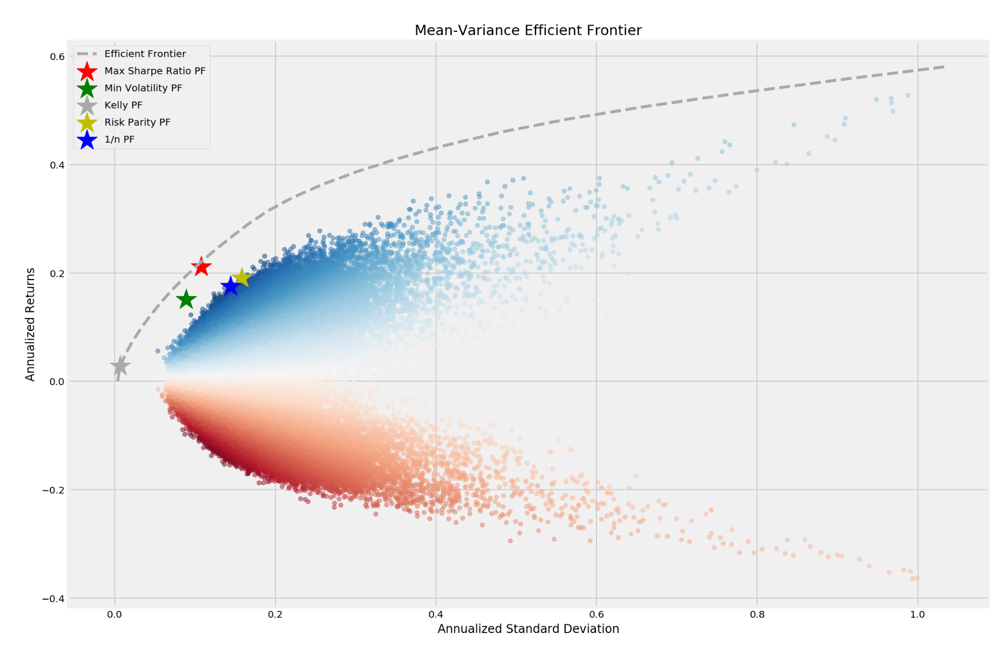
The simulation yields a subset of the feasible portfolios, and the efficient frontier identifies the optimal in-sample return-risk combinations that were achievable given historic data. The below figure shows the result including the minimum variance portfolio and the portfolio that maximizes the SR and several portfolios produce by alternative optimization strategies that we discuss in the following sections.

The portfolio optimization can be run at every evaluation step of the trading strategy to optimize the positions.