We will extend the univariate example of a single time series of monthly data on industrial production and add a monthly time series on consumer sentiment, both provided by the Federal Reserve's data service. We will use the familiar pandas-datareader library to retrieve data from 1970 through 2017:

df = web.DataReader(['UMCSENT', 'IPGMFN'], 'fred', '1970', '2017-12').dropna()
df.columns = ['sentiment', 'ip']

Log-transforming the industrial production series and seasonal differencing using lag 12 of both series yields stationary results:

df_transformed = pd.DataFrame({'ip': np.log(df.ip).diff(12),
                              'sentiment': df.sentiment.diff(12)}).dropna()

test_unit_root(df_transformed) # see notebook for details and additional plots

          p-value
ip          0.0003
sentiment   0.0000

This leaves us with the following series:

To limit the size of the output, we will just estimate a VAR(1) model using the statsmodels VARMAX implementation (which allows for optional exogenous variables) with a constant trend using the first 480 observations:

model = VARMAX(df_transformed.iloc[:480], order=(1,1), trend='c').fit(maxiter=1000)

This results in the following summary:

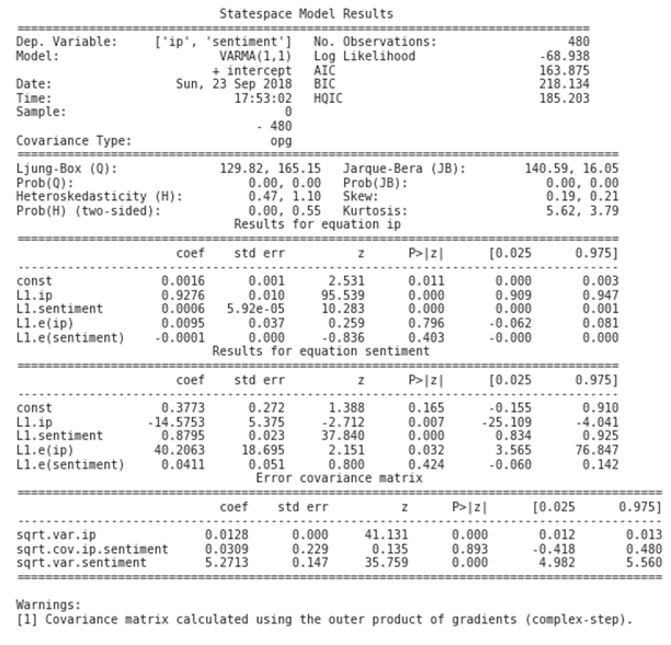
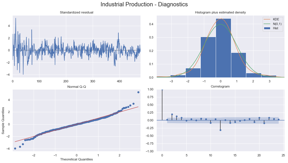
The output contains the coefficients for both time series equations, as outlined in the preceding VAR(1) illustration. statsmodels provides diagnostic plots to check whether the residuals meet the white noise assumptions, which are not exactly met in this simple case:

Out-of-sample predictions can be generated as follows:

preds = model.predict(start=480, end=len(df_transformed)-1)

A visualization of actual and predicted values shows how the prediction lags the actual values and does not capture non-linear out-of-sample patterns well: