In Chapter 7, Linear Models, we explored risk factor models used in quantitative finance to capture the main drivers of returns. These models explain differences in returns on assets based on their exposure to systematic risk factors and the rewards associated with these factors.

In particular, we explored the Fama-French approach, which specifies factors based on prior knowledge about the empirical behavior of average returns, treats these factors as observable, and then estimates risk model coefficients using linear regression. An alternative approach treats risk factors as latent variables and uses factor analytic techniques such as PCA to simultaneously estimate the factors and how they drive returns from historical returns.

In this section, we will review how this method derives factors in a purely statistical or data-driven way, with the advantage of not requiring ex-ante knowledge of the behavior of asset returns (see the pca and risk_factor notebook models for details).

We will use the Quandl stock price data and select the daily adjusted close prices of the 500 stocks with the largest market capitalization and data for the 2010-18 period. We then compute the daily returns as follows:

idx = pd.IndexSlice
with pd.HDFStore('../../data/assets.h5') as store:
stocks = store['us_equities/stocks'].marketcap.nlargest(500)
returns = (store['quandl/wiki/prices']
.loc[idx['2010': '2018', stocks.index], 'adj_close']
.unstack('ticker')
.pct_change())

We obtain 351 stocks and returns for over 2,000 trading days:

returns.info()
DatetimeIndex: 2072 entries, 2010-01-04 to 2018-03-27
Columns: 351 entries, A to ZTS

PCA is sensitive to outliers, so we winsorize the data at the 2.5% and 97.5% quantiles:

returns = returns.clip(lower=returns.quantile(q=.025),
upper=returns.quantile(q=.975),
axis=1)

PCA does not permit missing data, so we will remove stocks that do not have data for at least 95% of the time period, and in a second step, remove trading days that do not have observations on at least 95% of the remaining stocks:

returns = returns.dropna(thresh=int(returns.shape[0] * .95), axis=1)
returns = returns.dropna(thresh=int(returns.shape[1] * .95))

We are left with 314 equity return series covering a similar period:

returns.info()
DatetimeIndex: 2070 entries, 2010-01-05 to 2018-03-27
Columns: 314 entries, A to ZBH

We impute any remaining missing values using the average return for any given trading day:

daily_avg = returns.mean(1)
returns = returns.apply(lambda x: x.fillna(daily_avg))

Now we are ready to fit the principal components model to the asset returns using default parameters to compute all components using the full SVD algorithm:

pca = PCA()
pca.fit(returns)
PCA(copy=True, iterated_power='auto', n_components=None, random_state=None,
svd_solver='auto', tol=0.0, whiten=False)

We find that the most important factor explains around 40% of the daily return variation. The dominant factor is usually interpreted as the market, whereas the remaining factors can be interpreted as industry or style factors, in line with our discussion in Chapter 5, Strategy Evaluation, and Chapter 7, Linear Models, depending on the results of closer inspection (see the next example).

The plot on the right shows the cumulative explained variance, and indicates that around 10 factors explain 60% of the returns of this large cross-section of stocks:

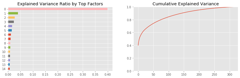
The notebook contains a simulation for a broader cross-section of stocks and the longer 2000-18 time period. It finds that, on average, the first three components explained 25%, 10%, and 5% of 500 randomly selected stocks.

The cumulative plot shows a typical elbow pattern that can help identify a suitable target dimensionality because it indicates that additional components add less explanatory value.

We can select the top two principal components to verify that they are indeed uncorrelated:

risk_factors = pd.DataFrame(pca.transform(returns)[:, :2],
columns=['Principal Component 1', 'Principal Component 2'],
index=returns.index)
risk_factors['Principal Component 1'].corr(risk_factors['Principal Component 2'])
7.773256996252084e-15

Moreover, we can plot the time series to highlight how each factor captures different volatility patterns:

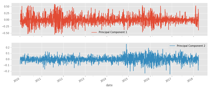
A risk factor model would employ a subset of the principal components as features to predict future returns, similar to our approach in Chapter 7, Linear Models – Regression and Classification.