2.2 ECONOMIC SCHEDULING PROBLEM CONSIDERING LOSSES

The economic dispatch problem is defined as that which minimizes the overall operating cost of all generators, C_T, of a power system while meeting the total load, P_D, plus transmission losses, P_L. Mathematically by the problem is defined as follows:

Where,

α_i, β_i, γ_i are the cost coefficients

P_i = real power generation by i^th generating unit (for i = 1, 2, …,).

n_g = Total number of generating units in power system.

Subject to the equality constraint the energy balance equation given as:

Where the total active power demand of n_b buses in the power system, and p₂ is the total transmission line power loss. Here P_Di Here P_Di is the active power demand for the i^th bus (for i = 1, 2, …) when subjected to the inequality constraint i.e., when power limits are imposed for the i^th generator;

where

One of the most important, simple but approximate method of expressing transmission loss as a funciion of generator power is through B-coefficients. Another more accurate form of transmission loss expression frequently known as the Kron’s loss formula

The constrained cost function Eq.(2.1) can be transformed into an unconstrained Lagrangian cost function by using the Lagrange multiplier as:

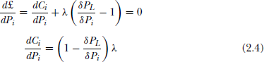
Where λ = Lagrangian multiplier Kuhn-Tucker condition. Differentiating £ with respect to P_i and equating to zero gives the condition for optimal operation of the system

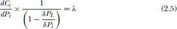
Using Eq.(2.5), the coordinate equations for n_g units can be written as:

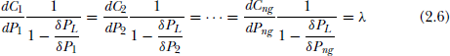
The general term in the Eq.(2.6) is written as:

Where L_i is known as the penalty factor of the i^th unit.

Where

   (for i = 1, 2, …n_g) is defined as the incremental transmission loss (ITL) associated with the i^th unit.

λ = Lagrangian multiplier also defined as the incremental cost of received power with units in Rs/MWh.

The Eq.(2.6) indicates that the minimum overall cost of generation can be obtained when the incremental fuel cost of each unit multiplied by its penalty factor is the same for all the n_g generating units.

Therefore Eq. (2.6) can be written as:

Where

incremental cost of generation of the i^th unit (for i = 1, 2, … n_g)

incremental transmission loss (ITL) associated with the i^th unit. (for i = 1, 2, …n_g)

The optimum load allocation amongst the units, taking transmission system losses into account can be obtained by operating all the generators at a particular generation point at which Eq.(2.7), i.e. for all the units are the same. The penalty factor L of the units can be determined through incremental transmission loss ITL. To find ITL, we need to develope formula for transmission line loss. The iterative procedure for solving the economic scheduling problem will be presented later. We discuss the derivation of the transmission loss formula in the following section.