
1.2 CHARACTERISTICS OF THERMAL UNITS
The cost of power generation by any thermal unit depends upon its characteristics. Performance of any unit can be understood by studying the generator’s input–output characteristics and the cost curve. Characteristics of individual machines are drawn on graphs and later converted into suitable mathematical equations using curves fitting methods. These mathematical equations are used to solve the economic scheduling problem. The input of a thermal unit is expressed in kcal/hr in terms of heat supplied or in Rs/hr in terms of cost of fuel, while the output is expressed in of MW.
1.2.1 Input–Output or Heat Characteristic
Heat curve is a graph drawn between fuel input in Btu/h or kcal/hr and power output in MW on x- and y-axis respectively, typical curve for a thermal unit takes the form as shown in Fig. 1.1.
The slope of the curve at different powers can be calculated. The slope is defined as heat rate or incremental fuel rate which is the ratio of fuel input to the corresponding power output and has the units Btu/MWh or kcal/MWh.
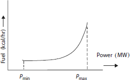
Fig. 1.1 Heat curve of a thermal unit
Incremental fuel rate = ![]()
Heat rate (slope of the heat curve) can be calculated at every point on the heat curve and another characteristic incremental heat curve can be obtained. This graph is drawn between incremental fuel rate in kcal/MWh and output in MW. The graph is shown in Fig. 1.2.
Incremental fuel characteristic is very important because it measures the thermal efficiency of a thermal unit and provides an estimate of fuel input needed for every additional MW generation. Different units have different incremental fuel rates for a given MW value. For optimal power generation, it is economical to allocate the load to the unit with minimum incremental fuel rate.
1.2.2 Cost Curve and Incremental Fuel Cost Characteristic
Knowing the specific heat (in kcal/kg) of the coal used, fuel input (in kcal/hr) and incremental fuel rate (in kcal/MWh) can be converted into kg/hr and kg/MWh respectively. Further, if cost of each kilogram of coal is known, then Kg/hr and Kg/MWh can be converted into Rs/hr and Rs/MWh.
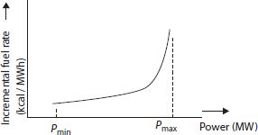
Fig. 1.2 Incremental fuel rate characteristic of a thermal unit
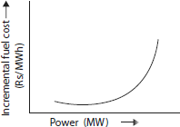
Now, the incremental fuel cost curve can be drawn by taking incremental fuel cost in Rs/MWh as an input on the y-axis and power in MW as an output on the x-axis. The cost curve is shown in Fig. 1.3.
Similarly, the input–output characteristic given in kcal/hr versus MW can be converted into a cost curve drawn as Rs/hr versus MW as shown in Fig. 1.4.
Let the fuel cost curve for the ith generator be in the form as shown in Fig. 1.4. The curve can be fitted in a quadratic equation as:
and incremental fuel cost can be written as:
Example 1.1
The fuel input characteristics for two plants are given by
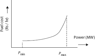
Fig 1.4 Cost curve of a thermal unit
where P1 and P2 are in MW.
- plot the input–output characteristic for each plant;
- plot the heat rate characteristic for each plant;
- assuming the cost of fuel as Rs 110/ton calculate the incremental production cost characteristics in Rs/MWh for each plant. Plot the characteristics against power produced in MW.
Solution:
- Input–output characteristic:
Consider the power in steps of 10 MW.
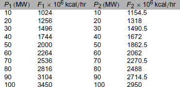
Fuel input characteristics are given as
F1 = (800 + 22 P1 + 0.04 P12) × 106 kcal / hrF2 = (1000 + 15 P2 + 0.045 P22) × 106 kcal / hrBy substituting P1 and P2 in the above equations, F1 and F2 values can be computed. The input-output characteristics are plotted in Fig. 1.5 (see Table 1.1).
- Heat rate characteristic:
Let P1 = 10 MW at Plant 1
Heat rate at this plant =

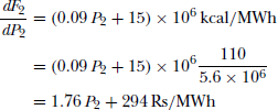
At Plant 2 P2 = 10 MW
Heat rate at this plant =

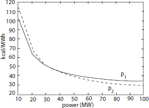
Repeat the above calculation for powers in steps of 10 MW till power at both the plants becomes 100 MW. This is shown in Fig. 1.6. (Table 1.2)
Table 1.2 Heat rate calculations
Output MW Heat rate ×106 for Plant 1 kcal/MWh Heat rate ×106 or Plant 2 kcal/MWh 10102.4115.452062.865.93049.8649.684043.641.8504037.256037.2534.367036.2232.428035 231.19034.4830.5610034.529.5 - Incremental production cost characteristic:†
Calorific value of fuel in the plants is 5600 kcal/hr
Cost of fuel = Rs 110 per ton = Rs 110/1000 per kg
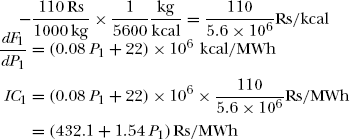
At 100 MW generation the cost is
IC1 = (432.1 + 1.54 × 200) = 740 Rs/MWh
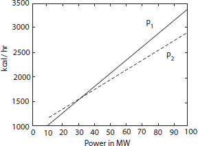
Fig 1.5 The inputñoutput characteristic curve
The incremental production cost is obtained by adding the maintenance costs of 10% (Table 1.3). Hence, the incremental production cost at Plant 1
At P1 = 10 MW
Similarly at Plant 2
Considering the maintenance cost at 10%
The incremental production cost at Plant 2 is
Table 1.3 Incremental production costs
| Power(P) | IPC at Plant 1 Rs/MWh | IPC at Plant 2 |
|---|---|---|
10
|
492.4
|
342.76
|
20
|
509.12
|
362.11
|
30
|
526
|
381.48
|
40
|
542.9
|
400.83
|
50
|
558.8
|
420.2
|
60
|
576.71
|
439.56
|
70
|
593.6
|
458.9
|
80
|
610.5
|
478.28
|
90
|
627.41
|
497.64
|
100
|
644.3
|
517
|
At P2 = 10 MW
In a similar fashion calculate IPC for all in steps of 10 MW till power is 100 MW. The characteristics are shown in Fig. 1.7.