
12
Electric Power Transmission and Distribution
OBJECTIVES: After studying this chapter, you will be able to
- Define and use terms used in the electric power industry
- Explain what a substation is
- Describe why it is necessary to transmit electricity at an elevated voltage
- Describe the difference between transmission and distribution
- Calculate the resistance of a length of wire
- Explain why transmission line conductors have inductance and capacitance
- Determine inductance and capacitance of transmission lines
- Describe what transposition in transmission line is and how it is done
- Select conductors carrying a given electric current under given conditions
- Explain why it is necessary to ground electric equipment
- Describe different ways that equipment can be grounded
- Use Thevenin’s and Norton’s theorems for solving network problems
- Use the principle of superposition for network problem solving
New terms: ampacity, bolt short circuit, circuit breaker, circular mil, corona, generator step up (GSU) transformer, geometrical mean distance (GMD), geometrical mean radius (GMR), grounding transformer, negative sequence, neutral grounding resistance (NGR), node, positive sequence, reactor, resistivity, specific resistance, substation, superposition, temperature coefficient, transposition, zero sequence
12.1 Introduction
Nowadays, in many large cities, electricity is provided by a grid that is powered by power plants that can be at a significant distance from the city. In modern countries, there are one or more grids for all electric power that are fed at various points where power plants are situated. For example, North America has three major grids: the Western Interconnection, the Eastern Interconnection, and the Electric Reliability Council of Texas (or ERCOT) grid. Larger power plants can be hydro, nuclear, or gas, oil, and coal fired. Wind and solar farms can be regarded as relatively small power plants. Also, there can be a lot of small hydro and diesel power plants that contribute to a grid power only during the peak hours.
Thus, a grid is an electricity power transfer carrier. Depending on its power transfer capacity and geographical extension, a grid can operate at various voltages, and as such, it must receive power from all generators feeding it and deliver to all consumers powered by it. This can imply transforming electric power from one level to another, sometimes several times, to be able to make connections. Even with only one power supply at one end of a grid and only one consumption location at the other end, it is necessary to raise the voltage from the generator site to a higher level and lower it after transmission at the consumer site. This is essential for the purpose of reducing energy waste and voltage drop, as demonstrated by Example 10.1 in Chapter 10.
In this chapter the pertinent matters associated with transmission and distribution of electricity and the necessary equipment are discussed.
12.2 Power Transmission and Distribution
Example 10.1 clearly demonstrated for a small load how the energy loss and voltage drop can be reduced by raising the voltage for transmission. This is, however, only possible to a certain limit, particularly at the level of consumer products. Operating voltage at domestic level in the world ranges from 100 V (in Japan) to 240 V (in the United Kingdom). This is the range accepted and operating in all countries (the operating voltages are 100, 110, 115, 120, 125, 127, 220, 230, and 240 V). From the production and distribution viewpoint, however, this is not an acceptable range at all. If the production, transmission and distribution are carried out at this low voltage, probably more than 98 percent of the production is lost in the transmission lines.
The reason is obvious. For the same power, if voltage goes up, current goes down. In this respect, both the voltage drop (IR) and the power used in the lines (RI2) decrease, as current decreases. Thus, the remedy is to increase the voltage for transmission as much as possible. Evidently, nevertheless, there is a cost involved and technical issues arise and how much the voltage can be increased is not an arbitrary choice. Different parts of a grid, moreover, can have different voltages.
Voltage chosen for a grid is based on decisions at the time of its construction but later on a grid can expand and integrate with other grids. The more common values for grid voltages are 34, 69, 138, 161, 230, 345, 500, and 765 kV. (Recently, a 1000 kV line was installed in China.) Table 12.1 shows the classification of the standard voltages in the United States.
Output of generators at large power plants is between 4000 and 20,000 V. This is further raised to a higher voltage, that of the grid, in one or more stages. Then, at the consumer site, the high voltage of the grid is lowered, again in one or more stages, before finally reaching houses and streets with a final stage when the voltage is lowered to one of the aforementioned values.
12.2.1 Substation
Substation: Point in the electric distribution network where transformers and switchgears are installed.
Raising or lowering line voltage is carried out in a substation. In addition, all switching, regulations, monitoring, and protection of the line take place in a substation. The main device for changing voltage is a transformer. The first transformer after a generator is the generator step up (GSU) transformer. Figure 12.1 shows a schematic of a small grid. This grid is fed only by one power plant. Larger grids have numerous feeding power stations. Any later installment to either feed this grid or take energy out of it must do so through a substation. In Figure 12.1, G represents a generator (power plant), GSU stands for generator step up, used for a stepping up transformer just after the generator to raise the generators voltage to that of the line it connects to, and CB denotes circuit breaker. A circuit breaker is an interrupter device as part of the protective means for part or all of a circuit. In case of malfunction or abnormal situations in a circuit, it cuts off electricity.
Table 12.1 Standard Nominal Three-Phase System Voltages per ANSI C84.1
| Voltage Class | Three Wire, V | Four Wire, V |
| Low voltage | 240 | 208Y/120 |
| 480 | 240Y/120 | |
| 600 | 480 Y/277 | |
| Medium voltage | 2400 | 4160Y/2400 |
| 8320 Y/4800 | ||
| 4160 | 12,000 Y/6930 | |
| 4800 | 12,470 Y/7200 | |
| 6900 | 13,200 Y/7620 | |
| 13,800 | 13,800 Y/7970 | |
| 23,000 | 20,780 Y/12,000 | |
| 34,500 | 22,860 Y/13,200 | |
| 46,000 | 24,940 Y/14,400 | |
| 69,000 | 34,500 Y/19,920 | |
| High voltage | 115,000 | |
| 138,000 | ||
| 161,000 | ||
| 230,000 | ||
| Extra high voltage | 345,000 | |
| 500,000 | ||
| 765,000 | ||
| Ultra high voltage | 1,100,000 | |
| 1,200,000 |
Generator step up (GSU) transformer: Transformer just after a three-phase generator in power generation plants that increases the voltage from the generator to match the voltage of the power line to the plant.
Circuit breaker: Same as a breaker, to disconnect a device or a circuit from power source to prevent damage.
In addition to transformers a substation is equipped with other devices for various functions. Among the devices in a substation are lightning arresters and air break switches. An air break switch is a switch for high voltages in transmission lines. Because opening and closing of these switches is accompanied by electric arc flash, it is necessary to suppress the arc. In an air break switch, compressed air is used for this purpose. Points A, B, C, and D in Figure 12.1 signify switchgear substations, where no voltage change takes place, but different branches meet.
As can be seen, a grid can have many circuit breakers at various points. Circuit breakers are of various types and they act based on some criteria, the existence of which are sensed by the appropriate sensors somewhere in the circuit. The action of sensors, normally called relaying, is set to

Figure 12.1
General representation of a simple electric grid.
measure and detect overvoltage, undervoltage, overcurrent, overfrequency, underfrequency, overtemperature, open phase, reverse power flow in motors, and so on.

Figure 12.2
Substation. (From Hemami, A., Wind Turbine Technology, 1E ©2012 Delmar Learning, a part of Cengage Learning Inc. Reproduced with permission from www.cengage.com/permissions.)
Figure 12.2 shows a small substation.
Electricity to houses and small buildings is single phase. In North America the nominal voltage for electricity in the buildings is 110 V (but depending on region and municipalities it can be between 110 and 125 V). Nevertheless, for certain appliances that need more power and take more current, such as the kitchen stove (range) and dryer, to lower current, the required voltage is 220 V (nominal). Common practice in North America is to deliver to each house a center-tapped 220 V line. The center-tapped line is grounded and acts as the neutral for building wiring. In this way, while 220 V is available for those devices that need it, the voltage difference between the center line and each other line is 110 V. Wiring for various parts of a house is almost evenly distributed between the two half voltage sources, and the stove and dryer are connected to the full voltage. Figure 12.3 shows the schematics of this wiring. This method of wiring is not practiced in other countries with 220 V electricity.
At this point it is worth noting that the special wiring of the lights for staircases and corridors that can be turned on-off by two switches at the two ends of the pathway. For this purpose, two DPST (double-pole single-throw; see Chapter 5) switches are used. Figure 12.4 shows this wiring scheme. It is also possible to turn a light on and off from more than two points. In this case the middle switch(s) must have four connections; each time, two alternative terminals pairs are connected together.
12.3 Electric Cables
Electric cables or conductors are basically of two types, but each type has numerous categories. Conductors are either for overhead transmission lines or for underground installation. Overhead conductors are bare wire and do not have insulation except at residential areas where contact with trees and other objects is possible, whereas underground conductors cannot be without insulation.

Figure 12.3
North American wiring scheme for residential buildings.
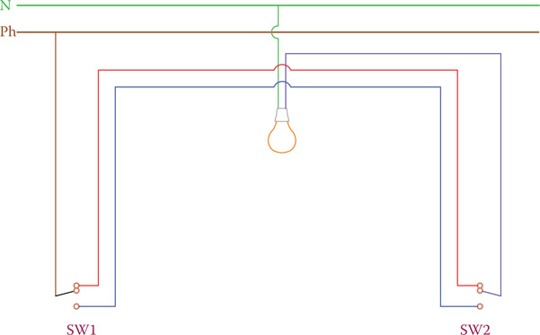
Figure 12.4
Two-switch staircase light wiring arrangement.
Overhead cables are cheaper because they do not have the problems with inclusion of insulation material and the required properties in their manufacturing process. But, they must be mechanically stronger because they are suspended from the poles/towers, and they must support their own weight, for which they must withstand a great tension. All conductors expand owing to heat generated in them when carrying current. This causes overhang conductors to sag more, which sometimes can result in contacts with lower lines or trees.
As we see in this chapter, we distinguish between transmission and distribution of electric power. Transmission is from the power plant to the consumer site where distribution takes place. Distribution takes place at different stages and at different voltages. Normally, the distribution lines conductors, for the low voltage that electricity comes to buildings, are made out of copper. Copper is heavier and more expensive than aluminum, which is an alternative for electrical wire material.
12.3.1 Overhead Conductors
For transmission lines nowadays the conductors are made of aluminum. Compared with copper, aluminum has less conductivity and less strength. For this reason, for the same power transmission, aluminum conductors must be thicker. Also, for overhead lines their strength can be reinforced by steel.
Theoretically, conductors can be made out of rigid bars. However, for transportation this is impossible and they should be flexible. See Figure 12.5. To increase flexibility of thicker conductors, they are made of several strands. As the current carrying capacity requirement of cables increases, more strands are added, and accordingly more reinforcement is necessary. The customary number of strands in overhead cables is as follows:
1 – 7 – 19 – 37 – 61 – 91, and 127
Note that each layer has six strands more than the layer inside it. For example, 19 = 1 + 6 + (6 + 6) and 37 = 1 + 6 + 12 + (12 + 6), etc. See Figure 12.6.
There are several categories of aluminum conductors. These are some of the more common aluminum conductors: all aluminum conductor (AAC), all aluminum alloy conductor (AAAC), aluminum conductor alloy reinforced (ACAR), aluminum conductor steel reinforced (ACSR), aluminum conductor steel supported (ACSS), aluminum conductor carbon fiber reinforced (ACFR), and gap-type aluminum conductor steel reinforced (GTACSR).
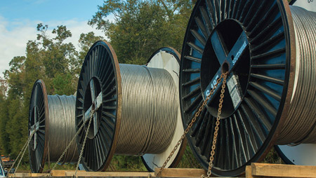
Figure 12.5
For various reasons including transportation, conductors must be flexible. (From ©2014 Southwire Company, LLC. All rights reserved. PPI reproduction is pursuant to Southwire Company, LLC’s express permission.)
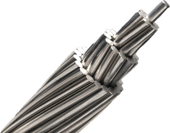
Figure 12.6
Typical bare wire conductor. (Courtesy of General Cable. ©General Cable Technologies Corporation, all rights reserved.)
There are other categories as well. The names are self-explanatory, to some extent, but can change from company to company. Not all conductors have strands with circular cross section. Figure 12.7 shows a cable with oval shape strands. Also, to increase the conductivity of cables for the same cross section, some cables have trapezoid shape strands that form circular layers, which resemble tubes of different diameters inside each other (see Figure 12.8). In this way, more use of space (thus, more conductivity) is made out of the same conductor diameter.
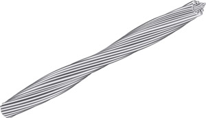
Figure 12.7
Conductor with oval cross section. (From ©2014 Southwire Company, LLC. All rights reserved. PPI reproduction is pursuant to Southwire Company, LLC’s express permission.)

Figure 12.8
Conductor with trapezoid strands. (Courtesy of General Cable. ©General Cable Technologies Corporation, all rights reserved.)

Figure 12.9
Aluminum conductor with composite core. (From ©2014 Southwire Company, LLC. All rights reserved. PPI reproduction is pursuant to Southwire Company, LLC’s express permission.)
More recently, carbon fiber reinforcement cables have been introduced; instead of steel, these cables have strands of carbon fiber composite material in the middle. Carbon fiber composite cable (CFCC) offers desired properties such as less weight and smaller thermal expansion compared with steel. It has 1/5 of the weight and 1/12 of thermal expansion of those of steel, for a price. Figure 12.9 shows a picture of such a cable.
A gap-type conductor consists of a core of high strength steel surrounded by a small gap filled with temperature resistant grease. Stacked around this gap are the trapezoid shape stands of aluminum.
In the seven-strand conductor there are six aluminum strands around one steel cable. The number of steel strands depends on the specification of a particular conductor. For a 37-strand cable, there are 30 aluminum and 7 steel strands, but for the 61-strand cable the number of steel strands can be 7 or 19 and the rest are aluminum. There are always exceptions, and these depend on the manufacturer.
Electric poles and supporting structures come in different forms and sizes, mainly based on the voltage of the power they transmit. Some typical ones are shown in Figure 12.10. For the final distribution to consumers’ poles of approximately 12 m (40 ft) are used, and the height of larger structures varies between 18 and 42 m (60 and 140 ft).
12.3.2 Electrical Properties of Electric Wires and Cables
The principal electrical property of a piece of metal is the resistance R that it shows to the flow of electrical current. It is very important to know the resistance of electric conductors when they are used in electric circuits. Knowing R allows one to determine voltage drop and the energy transformed into heat in parts of an electric circuit, in motor windings, and so forth. In addition to this property, for wires and cables, there is another property that determines how much current is allowed to pass through a conductor. This property, called ampacity (made from the two words “ampere” and “capacity”), defines the current capacity of an inductor based on the heat that is generated owing to electrical current, the structure and material of the conductor, and ambient temperature. It is easy to understand, therefore, that whereas the resistance of a wire can be almost constant, its ampacity depends on the temperature and some other working conditions, and it cannot be a constant.
Ampacity: A word (name) made of Ampere and Capacity. It is used to define the current capacity of standard conductors (wires) in different working conditions for safe operation. Ampacity is determined based on the heat generated in a conductor due to the current through it.
Resistance of a piece of any material (even an insulator) to the flow of electricity is proportional to its length and inversely proportional to its cross-section area. So, for example, if the length of a wire doubles, its resistance doubles, but if cross section doubles, resistance halves. R depends also on the material; for example, copper is a much better conductor than iron. This is why wires are made up of copper and not iron. The effect of the material is designated by the Greek letter ρ (rho, pronounced ro), which represents the resistance of a piece of the material with specific dimensions. The value ρ is called the specific resistance or resistivity of a substance.

Figure 12.10
Various transmission line supports.
Specific resistance: Same as resistivity: the electric resistance of a specific size (based on the measurement system) of a metal or material.
Resistivity: Same as specific resistance: the electric resistance of a specific size (based on the measurement system) of a metal or material.
On the basis of the aforementioned discussion, resistance R of a piece of wire can be found from
| (12.1) |
where ρ is the specific resistance, l is the length, and A is the cross-section area of the wire. Table 12.2 shows the specific resistance of some metals and nonmetals in metric system. The numbers shown are for the measurements made at 20°C. For other temperatures, values must be corrected by using the temperature coefficients in column 3 of Table 12.2.
Table 12.2 also shows the conductivity of materials. Conductivity is the inverse of resistivity. It is an indicator of how conductive a material is. Its unit in metric system is, thus, 1/ohm-meter. Also shown in the table is temperature coefficient, which represents how much the specific resistance of a metal changes with temperature. This implies that ρ does not have a constant value. Values given in tables are usually for the resistivity at room temperature (20°C). The relationship to calculate specific resistance of a metal at a different temperature than that known is
| (12.2) |
where t2 is the temperature at which we need to know the specific resistance ρ2, t1 is the temperature at which the value is known (ρ1), α1 is the temperature coefficient at t1.
Temperature coefficient: Numerical value (positive for metals) representing how much the specific resistance of a material changes with temperature.
Equation 12.2 can be readily substituted by
| (12.3) |
where R1 is the known value of the resistance at t1 and R2 is the resistance at t2.
The variation of the temperature coefficient α can be found from
| (12.4) |
α0 is the temperature coefficient at zero degrees.
Table 12.2 Specific Resistance (Resistivity) of Some Metals and Insulators
| Material | Resistivity ρ, Ωm | Temperature Coefficient per Degree Celsius | Conductivity σ × 107/Ωm |
| Silver | 1.59 × 10⁻⁸ | 0.0061 | 6.29 |
| Copper | 1.68 × 10⁻⁸ | 0.0068 | 5.95 |
| Aluminum | 2.65 × 10⁻⁸ | 0.00429 | 3.77 |
| Tungsten | 5.6 × 10⁻⁸ | 0.0045 | 1.79 |
| Iron | 9.71 × 10⁻⁸ | 0.00651 | 1.03 |
| Platinum | 10.6 × 10⁻⁸ | 0.003927 | 0.943 |
| Manganin | 48.2 × 10⁻⁸ | 0.000002 | 0.207 |
| Lead | 22 × 10−8 | … | 0.45 |
| Mercury | 98 × 10−8 | 0.0009 | 0.10 |
| Nichrome (Ni, Fe, Cr alloy) | 100 × 10−8 | 0.0004 | 0.10 |
| Constantan | 49 × 10−8 | … | 0.20 |
| Carbona (graphite) | 3–60 × 10−5 | −0.0005 | … |
| Germaniuma | 1–500 × 10−3 | −0.05 | … |
| Silicona | 0.1–60 | −0.07 | … |
| Glass | 1–10,000 × 109 | … | … |
| Quartz (fused) | 7.5 × 10¹⁷ | … | … |
| Hard rubber | 1–100 ×1013 | … | … |
a The specific resistance of these nonmetallic materials highly depends on the impurities in them.
Specific Resistance
Specific resistance is electrical resistance of a specific size of a material, and it is shown by the Greek letter ρ. In the metric system, ρ is the resistance of a piece of metal (10 mm × 10 mm × 10 mm), that is 1 cm long and has a cross section of 1 cm2 (see figure below). Because in the metric system the units for the length and area are meter and square meter, respectively, ρ is defined in ohm-meter (Ω.m) so that when inserted in the relationship for resistance the resultant is Ω.
In the US customary system, ρ is defined by the resistance of 1 foot of metal with a cross section of 1 circular mil (CM). See Appendix D for the definition of circular mil. The unit of measurement for ρ, therefore, is ohm-circular mil per foot (Ω.CM/ft).
Circular mil: Unit for measuring the thickness (cross section) of wires. A CM is the area of a circle whose diameter is one mil (1/1000 of an inch).

Example 12.1
What is the resistance of a copper wire 50 m long and having a cross-section area of 16.78 mm2 (AWG 5 wire)?
Solution
The resistivity of copper is 1.6779 (10−8) ohm-m. Thus,
Example 12.2
If the specific resistance of copper in metric system is 1.6779 × 10⁻⁸ (Ω.m), find what is it in the imperial system (Ω.CM/ft).
Solution
We should calculate the resistance of a foot long (0.3048 m) of the cable with a diameter of 1 mil (1/1000 inch).
Diameter = 1 mil = 0.001 in = 0.0000254 m = 25.4 × 10⁻⁶ m
Thus, the specific resistance of copper in the imperial system is 10.11 Ω.CM/ft.
In the above example the number in the second bracket can be used for conversion between values of specific resistance in the metric system and in the imperial system. Note that in the above example and in Table 12.2, specific resistance is (Ω.m) but sometimes it can be given in (Ω.cm).
Noting that
shows that when the specific resistance of a material in the metric system is given in Ω.m and in the form of a number multiplied by 10–8, we may easily find its value in Ω.CM/ft by multiplying the first number by 6.
Table 12.3 shows the specific resistance of a few metals in the imperial system of measurements.
Specific resistance of a material in Ω.m in the form of (xxx)(10–8) can be converted to Ω.CM/ft by multiplying the portion xxx by 6. The inverse conversion is done by dividing by 6.
Example 12.3
The diameter of a lightbulb filament is 0.05 mm, and it is made out of tungsten with the specific resistance of 5.6 × 10⁻⁸ Ω.m at the room temperature. If the filament length is 5 cm, what is the resistance of the filament at the room temperature?
Solution
Length = 0.05 m
Radius = 0.025 mm = 0.025 × 10⁻³ m
Table 12.3 Resistivity of Some Metals in Ω.CM/ft
| Material | Specific resistance Ω.CM/ft |
| Silver | 9.6 |
| Copper | 10.3 |
| Aluminum | 17 |
| Gold | 14 |
| Tungsten | 33.8 |
| Nickel | 52 |
| Platinum | 66 |
| Constantan | 295 |
| Mercury | 590 |
| Nichrome | 675 |
| Carbon | 22,000 |
Example 12.4
The resistance of a piece of wire 10 ft long is 100 mΩ. If the wire is made out of copper, find its thickness in CM.
Solution
The specific resistance of copper in imperial system is 10.11 Ω.CM/ft. From Equation 12.1 it follows that
The diameter of the wire is
Example 12.5
A piece of tungsten wire has a circular cross section with a diameter of 22 mils. What length of this metal makes a resistance of 10 Ω?
Solution
Diameter = 22 mil = 0.022 in = 0.0005588 m = 5.588 × 10⁻⁴ m
Cross-section area = (3.14)(5.588/2)2(10–4)2 = 2.4525 × 10⁻⁷ m2
It follows from the resistance relationship that
Length in English units = 44.6 × 3.28 = 146.3 ft
Example 12.6
If the resistance of a piece of tungsten wire at 20°C is 5 Ω, what is its resistance at 1200°C?
Solution
From Table 12.3 we see that the specific resistance and the temperature coefficient α for tungsten at 20°C are respectively 5.6 × 10⁻⁸ and 0.0045. Applying those in Equation 12.2 leads to
The specific resistance is 6.31 times larger. The resistance is, thus, larger by the same ratio. Therefore,
R1200 = (5)(6.31) = 31.55 Ω
You realize that when a lightbulb is on, the temperature of the filament is much more than room temperature, and, therefore, the resistance of its filament is several times larger than when at room temperature.
The standard wire sizes are given in Table 12.4 for both aluminum and copper wires. Table 12.4 also indicates the electric resistance per 1000 m and 1000 ft of these wires. AWG stands for American wire gauge.
12.3.3 Insulated Conductors and Ampacity
In the previous section we discussed the resistance of materials to electric current. We learned that almost all conductors are from copper or aluminum, and those from aluminum are reinforced by steel to give them mechanical strength when hanging from electric poles and towers. We also noticed that the sizes of wires are standardized and one must select a size among those that are commercially available. A different question that needs to be answered is how much current is allowed for a particular conductor. Ampacity (ampere capacity) is the answer to this question. Ampacity determines how many amperes of electric current a conductor can handle safely.
Table 12.4 American Wire Gauge Table
Ampacity is determined based on the amount of heat generated in a conductor owing to the current and the fact that this heat must be taken away, so that the conductor temperature does not increase anymore beyond a certain safe level. Otherwise, the buildup of heat can cause a problem. In this sense, the ambient temperature and the nature of conductor and its surroundings are the parameters that affect the ampacity rating of a conductor. In this respect, the same cable has more ampacity when in the air than when in a conduit.
Figure 12.11 illustrates a three-conductor underground cable. These cables come in different sizes with one, two, and three conductors and various insulation materials. Good electrical insulation is absolutely necessary for underground cables.
Overhead lines are normally in the air and cooled by streams of free air, whereas the underground cables are either in a conduit or buried underground. Also, their insulation decreases the rate of cooling compared to bare wires. The ambient temperature can be –30°C or +30°C, for instance, and it can vary significantly from winter to summer. Selection of cables must be based on the worst case scenario and the highest ambient temperature.
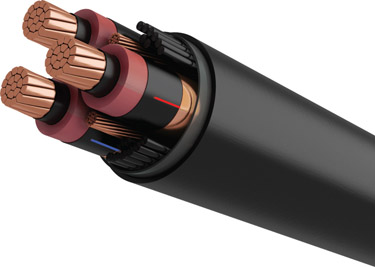
Figure 12.11
A three-conductor underground cable. (Courtesy of CME Wire and Cable, Inc.)
On the basis of the material and other conditions the ampacity of conductors are standardized. Tables 12.5 and 12.6 are examples of the ampacity of conductors according to National Electric Code (NEC) standard. These tables are only samples. Refer to NEC publications for a complete set of standards. Table 12.5 corresponds to ampacities of up to three conductors in a conduit, and Table 12.6 is for the same types of conductors when hanging in free air. In both cases the line voltage cannot exceed 2000 V.
As can be seen from these tables, ampacities are restricted for temperatures shown (30°C in this case) and must be adjusted for other temperatures based on the correction factors given in Table 12.7. The following examples show how these tables can be used. Letter combinations identified in the table are for the insulation types. Table 12.8 exemplifies the pertinent information. For full list of these types one must consult National Electric Code publications.
Example 12.7
Find the allowable current in a copper wire gauge AWG-8 for free air installation in an ambient reaching 45°C. The wiring is for 416 V (below 2000 V). Assume wire type TW.
Solution
From Table 12.6 we see three columns for copper wire. In the first column indicating TW and UF types, we find number 60 for gauge 8 wire. This implies that the maximum allowable current for this wire when the ambient temperature is 30°C is 60 A. For an ambient temperature of 45°C, however, this number must be adjusted by the coefficient given under “correction factors” in the same table. The corresponding factor for 45°C can be found to be 0.71. The maximum allowable current is, thus, 60 × 0.71 = 42 A.
Note that the ambient temperature may be less than 45°C most of the time, but one needs to consider the worst case when calculating the ratings.
Current capacity calculations for cables must be performed based on the worst case scenario.
Example 12.8
Determine the required wire gauge for 40 A current in a conduit where two of such copper wires are to be installed. The ambient temperature does not go over 38°C. The operating voltage is below 2000 V. Assume wire type TW.
Solution
From Table 12.7 we find that for temperature range 36°C–40°C a correction factor of 0.82 must be considered. If the desired current of 40 A is divided by this number, we get 40 ÷ 0.82 ≅ 50 A. Now we must find the standard wire corresponding to the
Table 12.5 Allowable Ampacities of Insulated Conductors in Conduits

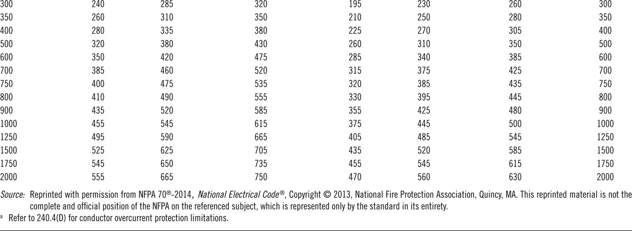
Table 12.6 Allowable Ampacities of Insulated Conductors in Free Air
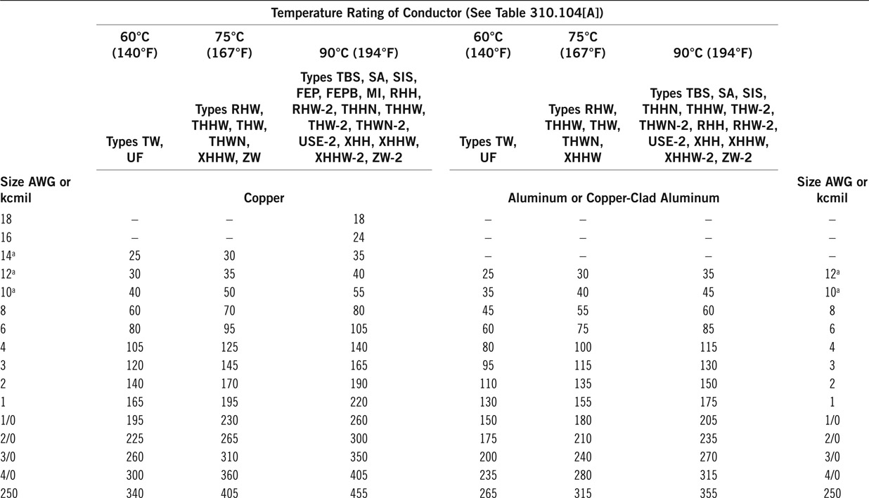
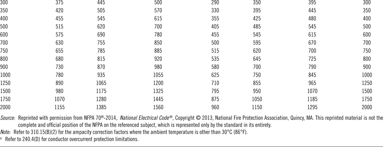
Table 12.7 Temperature Correction Factors for Tables 12.5 and 12.6
| Ambient Temperature (°C) |
Temperature Rating of Conductor
|
Ambient Temperature (°F) | ||
| 60°C | 75°C | 90°C | ||
| 10 or less | 1.29 | 1.20 | 1.15 | 50 or less |
| 11–15 | 1.22 | 1.15 | 1.12 | 51–59 |
| 16–20 | 1.15 | 1.11 | 1.08 | 60–68 |
| 21–25 | 1.08 | 1.05 | 1.04 | 69–77 |
| 26–30 | 1.00 | 1.00 | 1.00 | 78–86 |
| 31–35 | 0.91 | 0.94 | 0.96 | 87–95 |
| 36–40 | 0.82 | 0.88 | 0.91 | 96–104 |
| 41–45 | 0.71 | 0.82 | 0.87 | 105–113 |
| 46–50 | 0.58 | 0.75 | 0.82 | 114–122 |
| 51–55 | 0.41 | 0.67 | 0.76 | 123–131 |
| 56–60 | – | 0.58 | 0.71 | 132–140 |
| 61–65 | – | 0.47 | 0.65 | 141–149 |
| 66–70 | – | 0.33 | 0.58 | 150–158 |
| 71–75 | – | – | 0.50 | 159–167 |
| 76–80 | – | – | 0.41 | 168–176 |
| 81–85 | – | – | 0.29 | 177–185 |
Source: NFPA 70®-2014, National Electrical Code®, Copyright © 2013, National Fire Protection Association, Quincy, MA. Reprinted with permission. This reprinted material is not the complete and official position of the NFPA on the referenced subject, which is represented only by the standard in its entirety.
Note: For ambient temperatures other than 30°C (86°F), multiply the allowable ampacities specified in the ampacity tables by the appropriate correction factor shown above.
given conditions and with 50 A ampacity. We need to look in Table 12.5 under the column for the type of wire TW, but this ampacity of 50 A cannot be found in the table. Hence, we need to choose the gauge corresponding to the higher current of 55 A. The required wire is, thus, gauge 6.
12.4 Fault Detection and Protective Measures
Faults in an electric system can happen because of various reasons. Some faults in electricity distribution are due to natural causes such as lightning and are inevitable. Others can be due to deterioration of components as a result of age or abuse, and so on. What is important in operation is to detect a fault when it happens and have a proper action to prevent the harmful consequences, such as fire, damage, and destruction of equipment. In this section, as far as the scope of the book allows, electric faults in a power system are discussed.
12.4.1 Electric System Faults
In a three-phase power system, a fault, in general, can be a result of a short circuit or an inadvertent open circuit in one or two of the phases. A short
Table 12.8 Example of Definitions for Various Insulated Cables
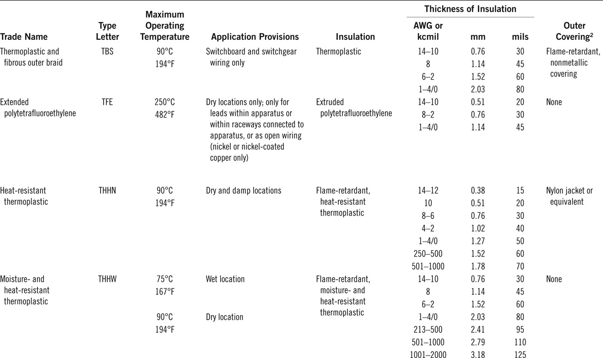

circuit can happen owing to physical wear of insulation as a result of age, thermal stress and fatigue, high voltage, high current, harsh environment, abuse, and the like. An open circuit can occur owing to lightning, overload, load surge, malfunction of a device, loss of synchronization, and so on. In either case, there is a significant imbalance between the currents in the three phases.
Depending on the severity of a fault, currents of several times magnitude can flow through wires, transformers, and a generator on the power side. If the fault persists, it can cause other failures in a system by over-heating and damaging parts, wires insulations, and insulators. In a power system it can cause fire or in the best situation if the protective devices act right and cut off the electricity (clearing the fault), a lot of consumers will be left without electricity until the cause of the fault is found and removed. In a bolt short circuit, that is, when a current carrying line is solidly shorted without any impedance in between, currents of several hundred times are not uncommon.
Bolt short circuit: Short circuit by direct contact between two lines of different voltages.
A fault in a power system is in one of the following forms: one phase shorted to ground, two phase lines shorted together, two phase lines shorted to ground, all phases shorted to ground, one line open, and two lines open.
In the case of any of these faults, if a system is not provided with the proper protective means, the consequences are costly. The importance of a protective measure is realized when a fault occurs. Thus, to reduce the risk of losing a power system and its equipment, or the electrical equipment in a consumer site, each side (generation and consumption) needs to be protected by the proper means. At the very lowest level and very fundamental to all protective means is grounding of an electric circuit at the source and at the consumption sites.
12.4.2 Grounding
Grounding is the major feature of the protective means for a power system, an electric device, and personnel. The other feature is clearing a fault, which is done by devices that break a circuit and clear the fault by removing the faulty device or portion of the circuit containing a fault.
For equipment, grounding causes the fault currents find their way through ground, and not through the equipment parts and windings. For personnel, grounding causes the voltage of a faulty equipment frame/case to stay at the ground level, so that if a person touches the frame, there is no potential difference between the body part in contact with the equipment and the ground.
Grounding implies physically connecting a point of a device or circuit to the earth, which provides a common reference point for zero voltage and a path for return of a current that otherwise has no path to flow through, to the source. For a power system, grounding is connecting the neutral point of the system to the earth, and for equipment, grounding implies connecting the noncarrying conductive material(s) such as motor frames and enclosures to earth.
In normal operation of electric systems the current through ground is negligible. This current may be due to unbalanced loads in a three-phase system, but it is still relatively small, especially that the soil resistance comes into effect. It is only when a fault happens that the connections to ground and the earth play their role in the currents that seek a path to follow. In such a case a high current is flowing in the ground wire of a grounded system. Table 12.9 shows the specific resistance of various earth materials.
For most electrical equipment, grounding is performed by a solid or bolt connection to ground, whereas for a system, such as the electric network, generators (like in all wind turbines), and in larger and expensive equipment, grounding can be either solidly or through a current limiting device (see Figure 12.12).
Neutral grounding resistance (NGR): An added resistance to the grounding strap to limit the (otherwise high) current flow through a device or a circuit in case of a fault.
Table 12.9 Specific Resistance (Resistivity) of Soil
| Type of Soil | Specific Resistance ρ, Ωm |
|
|
|
| Loam | 1–50 |
| Clay | 20–100 |
| Sand and gravel | 50–1000 |
| Surface limestone | 100–10,000 |
| Shale | 5–100 |
| Sandstone | 20–2000 |
| Granites, basalt | 10,000 |
| Slates | 10–100 |
Figure 12.12
Neutral Grounding Resistor.
The purpose of a current limiting device is to reduce the current that will flow through a device, and a system or its parts in case of a fault, which can cause damage. A common current limiting device for this purpose is a neutral grounding resistance (NGR). Such a resistor, nonetheless, must be carefully selected based on a number of criteria including the involved voltage and the allowed delay for the protecting device (e.g., a circuit breaker). A low resistance neutral grounding or a high resistance neutral grounding can be employed. In the former, the allowed current is higher. A current of 50 A or more (up to 400 A) is allowed for 10 sec. In the latter the maximum allowed current is 25 A for potentials of 600 V or less. A current of 5 A is more common. For higher voltages (13.8 kV and up), solid grounding is normally employed.
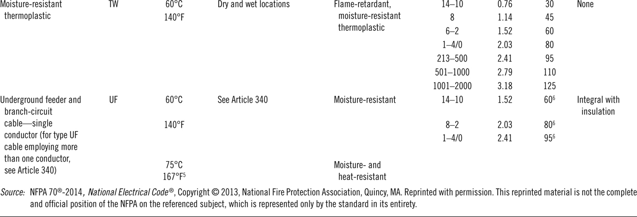
Figure 12.13
Using a single phase transformer in conjunction with a grounding resistor.
Instead of directly connecting a grounding resistor to the ground bus, a single-phase transformer can be employed, as shown in Figure 12.13. In this case a smaller resistor is used based on the transformer turns ratio.
It is important to have the grounding point on the secondary of a grounding transformer and as near to it as possible.
Recall from Chapter 8 that, as its specific property, an inductor resists a change in the current through it. This property makes it a candidate for current limiting, so it is desirable for grounding. As another means for grounding, a reactor can be used. A reactor is a winding (inductor) with or without a core, dry or oil immersed, which is specifically designed for a number of purposes, including grounding. Among other reactor applications are inrush-current limiting (for capacitors and motors), harmonic filtering, reactive power compensation, reduction of ripple currents, damping of switching transients, flicker reduction, load balancing, and power conditioning.
Reactor: Wire winding with or without a core, dry or oil immersed, which is specifically designed for a number of purposes, including grounding in a three-phase system.
12.4.2.1 What Point Must Be Grounded?
So far, we have talked about grounding. But, what point must be grounded? As we discussed in Chapter 9, the center point in a star connection of three-phase systems has a zero voltage with respect to all the phase lines. This point is, thus, a good reference for grounding. This is a point that, when it exists, it is grounded in all power facilities. When this point does not exist, in a delta connection, for example, such a point is created by an auxiliary transformer.
When this point is grounded in the source, and the loads have a similar point grounded, these points are connected to each other through the earth and any current coming from the load to ground finds its return way to the source through the earth. This can be a small current in the case of unbalanced three-phase loads, or a high current in the case of a fault. Remember that a substation is a load to a generator or to an upstream substation. In the same fashion a substation is a source for the loads or for a downstream substation.
In a grid, each line must be individually protected from faults.
12.4.2.2 Grounding in Power Transmission
We have seen in Chapter 10 that three-phase transformers can be used in four different configurations (see Section 10.6). These are delta-delta, delta-wye, wye-delta, and wye-wye. Each of these combinations has its advantages and disadvantages. A wye connection provides a suitable point for grounding. A delta connection provides a path for capturing third-order harmonics, which is quite important in power transmission and distribution.
Grounding transformer: Transformer used only for providing a reference point for connection to ground, in order for detection of faults in power generation and distribution.

Figure 12.14
Common arrangement for generators in traditional power plants.
It is more common to have one side delta connected and the other side wye connected to benefit from both advantages. However, it might be necessary to use a grounding transformer for the side with delta connection. The standard configuration by utilities for power transmission is “delta high – grounded wye low.” This implies that the higher voltage side is delta connected and the lower voltage side is star connected and it is grounded. This has the advantage that the low voltage bus has always a ground reference. Moreover, the common practice in traditional power plants (thermal and hydraulic plants) is to have the generator-step-up (GSU) transformer delta connected at the generator side (lower voltage) and the transformer secondary star-connected and grounded. A grounding transformer is then used for the generator to provide a solid ground for fault protection. This is depicted in Figure 12.14. A grounding transformer must have the correct size and rating for its purpose. Thus, its selection must be based on a careful study, and it is an additional cost to any facility.
In wind farms, however, because there are many wind turbines in a wind farm, the transformer at the generator side is star connected and grounded and the collector side (high voltage) is delta connected.
The standard configuration by utilities for power transmission is “Delta high – grounded wye low.”
A grounding transformer is a special wye-delta transformer that is designed for this purpose only. The secondary is not connected to any load and the primary is connected to the three-phase line at the location the grounding is desired. In the case of significant unbalance primary currents (a fault), very high currents circulate in the secondary windings. The transformer, therefore, must have been designed and rated for handling the high currents.
Also, a zigzag transformer can be used for grounding. The description of a zigzag transformer is given in Appendix C.
A grounding transformer is a special wye-delta transformer with its secondary not connected to any load. It is designed for the purpose of grounding only.
12.5 Transmission Lines
This section briefly describes matters concerned with transmission lines in electrical networks. Knowledge of the material described here is very useful for the technical personnel in electricity and its generation and distribution. Nevertheless, a thorough discussion of the subjects is out of the scope of this book, and the enthusiast reader must refer to other sources.
12.5.1 Transmission Lines Effects
In addition to the ohmic resistance in the wires and electric conductors, which we have discussed in this and Chapters 4–6, conductors carrying AC electricity have inductive and capacitive effects. Consider, for instance, a pair of transmission lines that extend for several miles and compare them to two plates forming a capacitor. You will see that there is a similarity in terms of the two metallic surfaces, being at a distance from each other, with a common cross-section area separated by a non-conductive material (air). Thus, the two conductors form a capacitor. The same thing is true for the magnetic effect of the current in each conductor on itself and on the other conductor. Thus, there exists inductance between the two conductors.
The amount of capacitive and inductive effects might be small and negligible for short wires, for example, in the household wiring having a low voltage, but they are not negligible for the very long transmission lines and the high voltages they carry.
Capacitive and inductive effects of the transmission lines, thus, need to be included in the calculation of their current and voltage drop. If these effects are added, the schematic representation of an electric network between load(s) and the source(s) is similar to Figure 12.15b, instead of Figure 12.15a. Resistances and inductances are in series with each other along the length of a conductor, but the capacitive effects are shown as parallel. These effects are indicated for one line only, but they correspond to both conductors. In practice, there are usually more than two conductors, particularly for three-phase lines. But, for three-phase systems the effects of two conductors do not add up as in the case of single-phase wires because there are no return lines carrying the exact same currents at the same moment.
Values for ohmic resistance can be readily defined for each conductor in terms of its length, cross-section area, the conductor material, and its specific resistance. These data are usually available for any cable in terms of the resistance for each meter of the conductor, or 1000 ft of it, as we have seen in the tables in Section 12.3.3.
Capacitor value and inductor value for a set of conductors, however, depend on the factors particular to their setup. Depending on conductors spacing, their radii, the way they are laid out, the number of conductors, and how many are in each bundle sharing the same current, a value can be determined for the inductance of a given length (e.g., 1 km or 1 mile) of a transmission line. Similarly, a value can be obtained for the capacitance. In this way, more precise values for the current, voltage drop, lost energy, and so on can be found for a transmission line of a given length.
Another phenomenon that causes loss in transmission lines is corona. Corona is the effect of potential difference (voltage) on the air surrounding the transmission lines, ionizing the air. This effect reflects in the form of a glow coming out of lines. Corona depends on the voltage and spacing between the wires. The amount of energy lost this way, however, is small and is often neglected.
Corona: Corona is a local electric discharge around the conductors of high-voltage transmission lines, when the (especially humid) air is ionized. It is manifested by a bluish glow and a small humming sound. This phenomenona is accompanied with a slight loss of power used for making the sound and the glow.

Figure 12.15
Typical representation of a transmission line. (a) Two long transmission wires for AC. (b) Assumed capacitors and inductors to represent the capacitance and inductance effects of the nearby wires in AC transmission.
Details of calculation of the equivalent inductor and capacitor for various line arrangements and spacing conditions is lengthy and involves mathematics that are out of the scope of this book. We may only use the results accompanied by some examples. To comprehend the subject, never theless, a reader is expected to have acquaintance with logarithm of a number because all calculations involve natural (or Naperian) logarithm (see the boxed text in this chapter for logarithm).
Figure 12.16 illustrates the relative spacing of possible transmission lines arrangements (compare with Figure 12.10). Figure 12.16a shows a general case where the three lines of a three-phase system are at locations 1, 2, and 3. These lines, furthermore, are at general distances D12, D13, and D23 from each other. In the discussions that follows it is assumed that the loads on the three phases are the same and we are dealing with balanced loads. Except in the case of Figure 12.16c where all lines are equidistance from each other, values for the inductance and capacitance of a length of the lines are not the same. As a result, voltage drops in the three lines are different. Consequently, at the load site the voltage at the three lines carrying three phases are not the same. Also, the phase relationships can be disturbed and the three phases will no longer be 120° from each other.
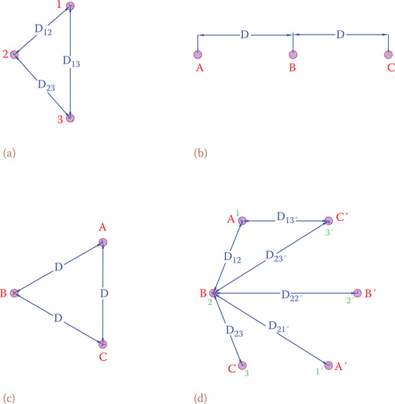
Figure 12.16
Conductor positions in some common three-phase transmission lines. (a) In three corners of a triangle. (b) Along one horizontal line. (c) At the three corners of an equilateral triangle. (d) Double-circuit three-phase, as on transmission structures.
It is very undesirable if the voltages arriving at a site from the same source are different and a proper three-phase system is not delivered at the line end. In many arrangements for transmission lines, it is not common, and sometimes impossible, to have the lines at the corners of an equilateral triangle (e.g., Figure 12.16b and d). To overcome this problem, it is common practice to rotate the lines, so that each of the phases occupies the same physical position equally along the length of the transmission line. In this way, the total inductance and capacitance of all three lines will be equalized. This rotation is called transposition, and a line treated this way is said to be transposed. This is illustrated in Figure 12.17, which illustrates that each of the three-phase lines A, B, and C are placed equally in the three physical positions denoted by 1, 2, and 3 along the length of the transmission line. When all the three phases of a line equally occupy the three positions, so that all the voltage differences cancel each other, the line is said to be completely transposed.

Figure 12.17
Transposition in transmission lines. (a) Physical position of the three-phase lines. (b) Interchanging the wire positions at some point along the line.
Transposition: Special arrangement in the transmission of three-phase power, in which the wires are rotated such that the location of wires for each phase is physically interchanged so that each wire equally occupies the same location as the other wires within the length of a line.
In all that follows we assume that the lines are solid, circular, and all have the same radius r. The distances are denoted by D with one or two indexes when necessary (like in D12). The numbers calculated for inductance and capacitance are for a given length, and, thus, for the whole length of a transmission line they must be multiplied by the line length. Results of the calculations are per phase for three-phase lines. In single-phase systems the numbers must be doubled for inductance and halved for capacitance because there are two lines and one is the return of the other line.
Before going ahead we need to define the two following terms. In fact, these are the parameters that change, from one line arrangement to another. Geometrical mean distance (GMD) is a number corresponding to the equivalent distance between two or more lines (cables). Geometrical mean radius (GMR) is a number corresponding to the effective radius of one or more lines.
Geometrical mean distance (GMD): A term in power transmission lines corresponding to the spacing between the two (in single phase) and three or six (in three phase) power lines used to determine the inductance and capacitance associated with lines.
Geometrical mean radius (GMR): Term in power transmission lines corresponding to the size (radius) of power lines used to determine their associated inductance and capacitance.
12.5.2 Line Inductance
The following general formula can be used for finding the inductance of each line in a transmission system. If three phase, the line is assumed to be transposed and the load(s) balanced.
| (12.5) |
GMD and GMR are as defined above, and they vary on a case-by-case basis. The coefficient (2 × 10⁻⁷) is for metric system, and the answer is in henries per meter. For the imperial system a conversion is necessary, as
Using logarithms is a useful tool in many engineering and other subjects. It makes calculations and solution to problems easier. Here we briefly explain what a logarithm is and show some examples. There are two logarithms, and we may say any positive number has two logarithm values. The difference between them is the base number, and it is possible to change from one logarithm to the other.
The two logarithms are decimal logarithm, which has a base 10, and the natural logarithm whose base is another number. We first start with the decimal logarithm, and when you understand it well, it is easy to understand the other. Indeed, logarithm is the opposite of exponential power.
Decimal Logarithm
To show the decimal logarithm of a number, the symbol “log” is used, such as log 10, log 20, etc. Consider the following relationships. You may want to check them on a calculator:
100.1 = 1.2589
100.2 = 1.5849
100.3 = 1.9953
100.5 = 3.1623
101 = 10
102 = 100
102.5 = 316.23
103 = 1000
In conjunction with the above relationships and in the same order you can write
Log 1.2589 = 0.1
Log 1.5849 = 0.2
Log 1.9953 = 0.3
Log 3.1623 = 0.5
Log 10 = 1
Log 100 = 2
Log 1000 = 3
From the above examples it is clear that if y = 10x, then x = log y.
Now that the notion of logarithm function is clear for you, try some negative numbers for the x and see the result on y. All values found this way are smaller than 1.0. Also, remember that negative numbers do not have logarithm. You will get an error message if try to find the log of a negative number on the calculator.
Natural or Naperian Logarithm
Instead of 10, the base for the natural (or Naperian) logarithm is the following number, which is denoted by e (always lowercase). You can see it on a calculator keyboard.
The symbol for natural logarithm is ln, like ln 10, ln 20, etc. The following show some examples for natural logarithm.
| e0.2 =1.221 | ln 1.221 = 0.2 |
| e0.5 =1.649 | ln 1.649 = 0.5 |
| e0.7 = 2.01 | ln 2.01 = 0.7 |
| e1 = 2.718 | ln 2.718=1 |
| e2.3026 = Q | ln 10 = 2.3026 |
| e4.605 =100 | ln 100 = 4.605 |
| e−0.2 = 0.8187 | ln 0.8187 = −0.2 |
| e−1 = 0.3679 | ln 0.3679 = −1 |
There are a number of useful rules for using logarithm, but we restrict this discussion and leave them out. You can find all those in a mathematics book. You notice that for negative powers the answer is smaller than the base. Also, notice the relationship between the two logarithm values
ln x = 2.3026 log x (x can be any positive number)
log x = 0.4343 ln x
will be seen later in some examples. We consider GMD and GMR for the following three cases:
- Case of single phase (two lines):
GMD = D = the distance between the lines
where r is the wire radius. Because in this case the return line has the same characteristic and current as the main line, the value obtained for L must be doubled to represent the closed loop.
For single-phase lines the values calculated for inductance from Equation 12.5 must be doubled.
-
2. Case of three-phase single circuit line (Figure 12.16a, b, and c):
For all of the above cases
(12.6) (12.7) (D12, D13, and D23 are the distances between lines as shown in Figure 12.16, r is the radius of the cables.)
-
3. Case of double circuit three-phase lines (Figure 12.16d):
Note the way numbers and letters are assigned to the three-phase lines, and the definition of various distances.
(12.8) where
(12.9) where
(12.10)
The values obtained from the preceding relationships determine the inductance of each line of a three-phase system. The values are in henries per meter.
Note that Thus, in all the above equations, this value can be directly used (e = 2.7183).
After L is determined, the inductive reactance of the line is determined from the familiar relationship XL = 2πfL.
(For all distance definition between lines, see Figure 12.16d; all lines are assumed to be the same size with a radius r.)
Values obtained for L and XL are per meter of each line. For the inductance and inductive reactance of the entire line, they must be multiplied by the line length.
Example 12.9
Find the inductance for a pair of single-phase lines, where their distance is 2.5 ft and their diameter is 0.2576 in (gauge 2 wire). What is the inductive reactance per mile of this line for 60 Hz electricity?
Solution
D = 2.5 ft = 0.7622 m, r = 0.2576 ÷ 2 = 0.1288 in = 0.00327152 m
L = (2)(2 × 10–7 × 5.7) = 2.28 × 10⁻⁶ H/m (For single phase the value given in Equation 12.5 must be doubled.)
XL = 2πfL = (2)(3.14)(60)(2.28 × 10⁻⁶) = 0.86 × 10⁻³ Ω/m
(0.86 × 10⁻³)(1609) = 1.38 Ω/mile (1 mile = 1609 m)
(Note that because we calculate the logarithm of a ratio, as far as the two values have the same units, no further unit conversion is necessary.)
Three wires of 25 mm diameter are used in a transmission line arranged as shown in Figure 12.16b. If the distance D, as shown in the figure, is 2.5 m, find the inductance of the wire per phase and the inductive reactance for a completely transposed line 4 km long carrying 50 Hz electricity.
Solution
On the basis of the definition of the distances between the lines, we observe that
D12 = D23 = 2.5 m, D13 = 5 m, d = 25 mm, r = 12.5 mm = 0.0125 m
GMR = (0.7788)(0.0125) = 0.009735 m
L = 2 × 10–7 × 5.7794 = 1.1559 × 10⁻⁶ H/m
XL = 2πfL = (2)(3.14)(50)(1.1559 × 10⁻⁶) = 3.63 × 10⁻⁴Ω/m
For 4 km,
XL = (4000)(3.63 × 10–4 = 1.45 Ω
Example 12.11
A transmission line uses six similar conductors of 4 cm diameter, as shown in Figure 12.16d. If the vertical distance between each pair of adjacent wires is 3 m, horizontal distance for the adjacent pairs is 5 m and for middle conductors is 8 m (as shown in Figure 12.18), find the inductance of the line. The line is completely transposed.
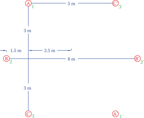
Figure 12.18
Wire position arrangement for Example 12.11.
Solution
We can do this calculation in four steps:
- Step 1: First, we need to find the distances between various lines, from geometry.
- D12 = = 3.354m
- D12′ = = 7.159m
- D1′2 = D12′ == 7.159m
- D1′2′ = D12 = 3.354m
- D13 = 3 + 3 = 6m D13′ = 5m
- D13′ = 5mm
- D1′3′ = D13 = 6m
- D23 = D12 = 3.354m
- D23′ = D12′ = 7.159m
- D2′3 = D12′ = 7.159m
- D2′3′ = D12 = 3.354m
- D11′ = 211 6 + 52 = 7.810m
- D22′ = 8m
- D33′ = D11′ = 7.810m
- Step 2: Find the equivalent values for DAB, DAC, and DBC and calculate GMD.
- Step 3: Find GMR from GMRA, GMRB, and GMRC.
GMRC = GMRA = 0.493 m
- Step 4: Find the inductance.
Example 12.12
If the wire in Example 12.9 has 0.1563 Ω resistance per 1000 ft, what is its impedance per mile?
Solution
Resistance per mile = R = (0.1563)(5280)(0.001) = 0.825 Ω
Inductance per mile = XL = 1.38 Ω (found in Example 12.9)
12.5.3 Line Capacitance
Line capacitance of electric conductors can be found in the same way that their inductances were formulated for various line arrangements. The only difference is in the value of geometric mean radius, as far as the formulas are concerned. In addition, the effect of the ground comes into picture for capacitance. However, this effect is only a small fraction of the values of capacitance due to the wires themselves and can be ignored unless the cables are very near to the ground.
The value of GMR in Equation 12.7 for the case of capacitance is the actual radius of the conductor. In this respect, for all the calculations of capacitance the term (when it appears in the equations for inductance) must be replaced by 1. The general formula for capacitance of conductors in the metric system is
| (12.11) |
and the answer found this way is in F/m (farads per meter). For any length of conductors this value must be multiplied by the length.
For the simple case of two wires, GMR is simply the radius of the wires and GMD is their distance. The following examples determine the capacitance for some of the same conductors as previously seen in this section.
The value obtained from Equation 12.11 is for the capacitance between each phase line and the neutral in a three-phase balanced system. For single phase the calculated value must be divided by 2 to find the capacitance between the hot line and neutral. In the above equation the effect of earth is assumed small and is not included.
Example 12.13
Find the capacitance for a pair of single-phase lines, where their distance is 2.5 ft and their diameter is 0.2576 in.
Solution
For the simple case of two wires GMD = distance between the two wires, and GMR = radius of each wire (assuming the same radius). Because this is for a single phase, the value obtained from Equation 12.11 must be halved or, instead, the multiplier 2 in the numerator should be dropped. Moreover, because the logarithm of a ratio is found, it is only necessary that the units for the numerator and the denominator be the same.
D = 2.5 ft r = 0.2576 ÷ 2 = 0.1268 in = 0.0105667 ft
C = (π × 8.854 × 10⁻¹²) ÷ (5.466) = 5.088 × 10⁻¹² F/m = 5.1 × 10⁻⁶ μF/m
For any 1 km of this line, capacitance is 0.0051 μF, and for each mile it is 0.0082 μF.
Example 12.14
A transmission line uses six similar conductors of 4 cm diameter, as shown in Figure 12.18, with the shown spacing between them. Find the capacitance of the line. The line is completely transposed.
Solution
The line configuration and size here are the same as in problem of Example 12.11. It is recommended that you refresh your memory about what was done there to determine the line inductance. Steps 1 and 2 of Example 12.11 can be repeated to find GMD. These are not duplicated here. The final answer is the same as obtained before:
A new GMR, however, must be found. GMR values for the three phases depend on the spacing D11′, D22′, D33′, based on Equations 12.10. These values also have been already determined in Example 12.11 and are
D11′ = D33′ = 7.810 m
D22′ = 8 m
Using these values in Equation 12.10, but without the factor 0.7788, leads to
GMRC = GMRA = 0.559 m
and the capacitance can be found to be
In practice, for medium length lines (typically 80–250 km, 50–156 mi) after the values of the resistance, inductive reactance, and capacitive reactance are found, the line is modeled as a π circuit or a T circuit, as shown in Figure 12.19. In the π circuit model, the capacitance of each capacitor is half of the total calculated value. Likewise, in T circuit the values of impedances are half of the calculated value.

Figure 12.19
Modeling of transmission lines. (a) π model. (b) T model.
12.6 Rules for Network Problems
Analysis of circuits described in Chapters 6 and 8 were for simple electric networks containing a combination of components that could be broken into series and parallel resistors (in DC) or RLC’s (in AC) and reduced to a final single loop. Not all the circuits are so simple and can be analyzed with only those rules. For example, most of the electronic circuits, at the small-scale voltage, and the power transmission and distribution in electrical grid, at the large scale, have more complicated circuits. For instance, consider the circuits depicted in Figure 12.20. None of these circuits can be simplified by the rules of series and parallel components. These circuits are characterized by having more than one loop. (Note that here we consider an RLC parallel circuit as one loop containing the three elements because we already know how to handle it).
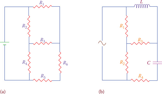
Figure 12.20
Examples of electric networks for the analysis of which we need new rules. (a) DC circuit. (b) AC circuit.
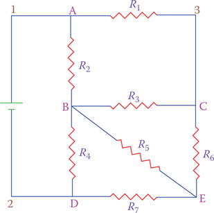
Figure 12.21
A circuit with multiple loops and nodes.
In this section we consider some additional laws and theorems that can be employed for more involved circuits and networks. The first step in all problems, however, is to reduce a circuit to its simplest form by the rules that we have already studied for series and parallel components. If the reduced circuit has only one loop, then the new rules will not be necessary. Otherwise, the new rules will be implemented to solve for the unknowns of the circuits.
In a circuit with more than one loop there nodes also exist. A node is a point in a circuit where three or more branches meet. Points A, B, C, D, and E in the circuit in Figure 12.21 are nodes. Quite a number of loops can be identified in this circuit. These are 1AD2, 13E2, A3CB, A3ED, BCED, BCEB, BEDB, A3CEB, 1A3CBD2, 1A3CED2, 1ABCED2, and 1ABED2. Not all of the loops contain the power supply (or a power supply in case there is more than one).
Node: Any point in an electric circuit where more than two lines (branches) join each other.
12.6.1 Kirchhoff’s Voltage Law
Problems similar to those in Figure 12.20a and b can be solved by employing Kirchhoff’s laws. We need to find some or all the currents in each of the seven resistances and/or finding the potential difference between various points, such as VAB, VAC, VBC and so on.
Kirchhoff’s voltage law states that the algebraic sum of all voltages across the components in a loop is equal to the algebraic sum of the source voltages (there might be more than once source) in the loop. Attention must be paid to the polarity and the sign of a voltage. This is the reason for stating algebraic sum because some of the values can be negative. The voltage sign in a component depends on the direction of the current. For clarity, this is shown in Figure 12.22a. For a source the voltage sign is negative for the direction toward the positive terminal.
For those loops that contain no source the sum of the voltages across the components is zero because there is no source, and, consequently, their sum is zero. In Figure 12.23, three loops out of six possible loops are shown. Application of Kirchhoff’s voltage law to these loops reveals that
VAC + VCE = 24
VAC + VCB + VBA = 0
VBC + VCD + VDB = 0
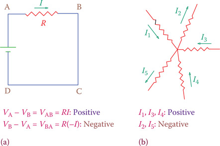
Figure 12.22
Voltage and current sign designation. (a) Voltage difference signs for a loop. (b) Current signs for a node.

Figure 12.23
Loops and currents in a network.
An alternative way of expressing Kirchhoff’s law is “The algebraic sum of all the voltages in a loop is equal to zero.” This statement involves the sign assignment for all components including the sources.
The sum of all the voltages in a loop is equal to zero considering a positive sign for the voltage in a forward direction of current and negative in the reverse direction of current for all components but opposite to this for the sources.
12.6.2 Kirchhoff’s Current Law
Kirchhoff’s current law states that the algebraic sum of all the currents in a node is zero. In other words, the sum of all currents coming to a node is equal to the sum of all currents leaving it. The currents coming toward a point are considered positive and the currents leaving the node are considered negative, as depicted in Figure 12.22b.

Figure 12.24
Circuit, for example, of Kirchhoff’s laws application.
In the circuit of Figure 12.23, there are five resistors and each one has a different current. Applying the Kirchhoff’s current law to nodes A, B, C, and D reveals that
At A, I1 + I2 = I (circuit current)
At B, I3 + I4 = I2
At C, I1 + I3 = I5
At D, I4 + I5 = I
The Kirchhoff’s current law defines the relationships between various currents in a circuit because these currents are not independent of each other. In this sense, in the circuit of Figure 12.23 one can assume only three unknown currents I1, I2, and I3 because I4, I5, and I may be defined in terms of I1, I2, and I3, as shown in Figure 12.24. The following example shows the application of Kirchhoff’s voltage and current laws.
The algebraic sum of all the currents in a node is equal to zero, considering the currents toward a node as positive and currents leaving a node as negative.
Example 12.15
In Figure 12.24, find the current in the circuit and the voltage at point B (assuming voltage at D is zero). All the resistor values are in Ω.
Solution
Various loops and currents can be defined for any such problem but all lead to the same solutions. A set of currents are defined and shown in Figure 12.24. We need to write the Kirchhoff’s law for the selected loops. As there are only three independent currents, only three equations are necessary and sufficient.
| 140I1 + 40I3 = 24 | (From loop ACDEA) |
| 100I1− 120I2 + 40I3 = 0 | (From loop ACBA) |
| 40I1 − 68I2 + 40I3 = 0 | (From loop BCDB) |
Any known method can be used for the simultaneous solution of the above three equations. The results are
I1 = 170.0 mA
I2 = 128.8 mA
I3 = 4.90 mA
The total current in the circuit is
I1 + I2 = 298.8 mA
and the voltage at point B can be found from the voltage drop in the 120 Ω resistor to be
VB = 24 − (120)(0.1288) = 8.544 V
12.6.3 Thevenin’s Theorem
Thevenin’s theorem is particularly helpful when multiple power supplies exist in a circuit. In Figure 12.25, for example, there are two power supplies, and we need to find the current through the resistor R. This could be part of a larger circuit, which provides 12 and 6 V across the points shown in the figure. Refer to Figure 12.25 for understanding the statement of Thevenin’s theorem.
Thevenin’s theorem states that the current through a resistor R connected across any two points A and B in an active network is obtained by dividing the potential difference between A and B (with R disconnected) by R + r, where r is the resistance of the circuit between A and B (with R disconnected) and the sources of the circuit replaced by their internal resistances.
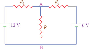
Figure 12.25
Application of Thevenin’s theorem.

Figure 12.26
Equivalent circuit by Thevenin’s theorem.
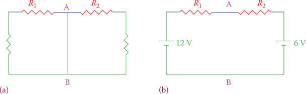
Figure 12.27
Steps in implementing Thevenin’s theorem. (a) Finding equivalent rTh between points A and B. (b) Finding the voltage difference VTh, between points A and B.
Active network implies that the circuit considered is not dead and has EMF sources within it (EMF implies a voltage source). The internal resistance of sources corresponds to resistances that may exist in the power sources but can be zero (see Appendix A).
In other words, Thevenin’s theorem implies that to find the current through R (or the voltage difference between A and B), replace this circuit by an equivalent circuit as shown in Figure 12.26. In this circuit, there are two unknown values of which need to be determined: the resistance r and the voltage V.
To find r,
- Disconnect R (see Figure 12.27a).
- Replace each voltage source by its internal resistance.
- Remove any current source.
- Determine the resistance between A and B.
To find V,
- Disconnect R (see Figure 12.27b).
- Find the voltage between A and B.
Example 12.16
Part of a circuit can be represented by three resistors and two power sources as shown in Figure 12.28. If R1, R2, and R (corresponding to Figure 12.25) are, respectively, 80, 120 and 32 Ω, find the current in the 32 Ω resistor and the voltage across it. The internal resistances of the sources are zero.
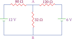
Figure 12.28
Circuit of Example 12.16.
Solution
By Thevenin’s theorem this circuit can be replaced by a voltage V and a resistor r, as shown in Figure 12.29a.
The resistor r can be found by following the three above mentioned steps. Because the source internal resistances are zero, the two branches in parallel with the 32 Ω resistor contain 80 and 120 Ω. Thus the resistor r is calculated as
or
r = 48 Ω.
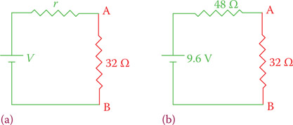
Figure 12.29
Thevenin’s circuit for Example 12.16. (a) Thevenin’s equivalent circuit. (b) Values for Thevenin’s model.

Figure 12.30
Finding voltage at A Thevenin’s equivalent circuit.
The voltage V may be calculated as the voltage at A (assuming VB = 0) based on a voltage drop in R1 (the 80 Ω resistor) in the circuit of Figure 12.30 (32 Ω resistor removed). The current in this circuit is
and the voltage drop in R1 is, accordingly, 80 × 0.03 = 2.4 V, which implies that the voltage at A is 12 − 2.4 = 9.6 V. The resulting circuit is indicated in Figure 12.29b. On the basis of this voltage and the resistor r (Thevenin’s equivalent circuit) the current through the 32 Ω resistor is 9.6 ÷ (48 + 32) = 0.12 A.
Thevenin’s theorem is not only for circuits with multiple sources. It can be employed for a circuit similar to that shown in Figure 12.23 (and solved by using Kirchhoff’s laws) when we are more interested to see the current in a resistor’s value is subject to change. If for various values of a resistor we assume we have to repeat all the calculation, it is tedious. By using Thevenin’s theorem we can readily find the current for each value of the resistor.
Example 12.17
For the circuit shown in Figure 12.24 and repeated in Figure 12.31a we want to find the equivalent Thevenin’s circuit as seen from the 40 Ω resistor.
Solution
The two points across the 40 Ω resistor are called M and N for referencing.
-
Find the resistor r: Shorting the two sides of the battery leads to the circuit shown in Figure 12.31b. We need to find the single resistor that is between points M and N, neglecting the 40 Ω resistor. This is shown in Figure 12.31b. We need to rearrange this circuit to a clearer form, so that it can be simplified and reduced to a single resistor. We note that points A and C are the same for this circuit; between M and A, there is a 100 Ω resistor; and there exists a 300 Ω resistor between M and B. The circuit in Figure 12.31b can be rearranged as shown in Figure 12.31c, which can be easily managed. Point M is shown twice for better clarity.
For these four resistors we can write
from which the value of r can be found as r = 77.45 Ω.
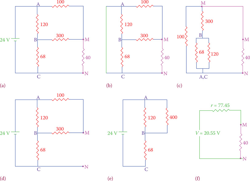
Figure 12.31 Steps for finding the Thevenin’s circuit in Example 12.17. (a) Original circuit. (b) Replacing voltage sources by their internal resistance. (c) Finding the total resistance across the load points. (d) Removing the load to find the voltage at load points. (e) Finding voltage difference across the load points (load removed). (f) Final result.
-
Find the voltage V: We need to find the voltage between points M and N when the 40 Ω resistor is removed. Removing this resistor from the circuit leads to that shown in Figure 12.31d, which can be further reduce to the circuit depicted in Figure 12.31e to find the voltage at point B assuming the voltage at C is zero (connected to the negative terminal of the battery). The voltages VAB and VBC can be found from the voltage divider relationships (see Chapter 6).
(93.3 Ω is equivalent resistance of 120 and 400 Ω resistors in parallel)
VBC = 24 − 13.8 = 10.2 V
We need further to find the voltage at point M. This voltage can be obtained by observing that in the branch containing the 100 Ω resistor and 300 Ω resistor the 13.8 V voltage is divided between these two resistors. The voltage at M, thus can be determined to be
which implies that VMN = 20.55 V.
The final result, the Thevenin’s circuit, is shown in Figure 12.31f.
As a test, let see the current in the 40 Ω resistor based on the above analysis. This current is equivalent to I1 + I3 in Example 12.15.
From Thevenin’s theorem:
I40 = 20.55 ÷ (77.45 + 40) = 0.175 A = 175 mA
From Example 12.15:
I1 + I3 = 170 + 4.90 = 174.9 mA
Consider, for instance, if the 40 Ω resistor has to be replaced by a 50 Ω resistor. The new current in this resistor is
I50 = 20.55 ÷ (77.45 + 50) = 0.161 A = 161 mA
12.6.4 Principle of Superposition
The principle of superposition is another useful method that can be used in many problems. It has a broad application in many topics. In the context of this discussion it can be employed for solving problems similar to those tackled by Thevenin’s theorem when multiple sources exist. The principle is that a problem is broken into a number of overlapping but simpler cases. At the end, the solutions of the various cases are combined together. In our case of two sources in the same circuit, we break down into two overlapping problems, each one dealing with the same circuit, but only one source. We solve the simpler problems, and at the end, we add up the separately found currents for each component. As an example, we consider the same problem in Example 12.16.
Superposition: A method of analysis of problems containing multiple parameters or conditions (inputs for example) by supposing that each parameter exists without the presence of the others, and then the different outcomes (of applying each parameter) are added together.
Example 12.18
Referring to Figure 12.28, repeated in Figure 12.32a, part of a larger circuit can be represented by three resistors and two power sources, as shown. Find the current in the 32 Ω resistor.
Solution
We first consider the circuit without the 6 V source. The resulting circuit is shown in Figure 12.32b. The corresponding current I1 in the circuit can be found as
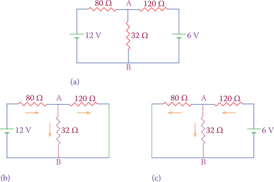
Figure 12.32
Separating the sources in the circuit of Figure 12.27. (a) Original circuit. (b) The 6 V battery is removed. (c) The 12 V battery is removed.
This is the current in the 80 Ω resistor due to the 12 V battery. Only part of this current (I1,32) flows through the 32 Ω resistor, which can be determined from the resistors’ ratio:
Next, we consider the circuit without the 12 V source and follow the same process (Figure 12.32c).
This is the current through the 120 Ω resistor due to the 6 V battery. The part I2,32 passing through the 32 Ω resistor is determined as
The total current through the 32 Ω resistor is obtained by adding the two partial currents. Therefore,
I32 = 0.090 + 0.030 = 0.120 A
This is the same answer as obtained by Thevenin’s theorem.
Thevenin’s theorem has the advantage that in case this resistor is subject to variation, we do not need to repeat all the calculation every time. We just simply enter the changed value of the resistor in the equivalent circuit.
The advantage of using Thevenin’s or Norton’s theorems is more pronounced when the value of a resistor is subject to change. It is not necessary to repeat all calculations every time for a new value of a variable resistor.
Note that the directions of the two currents to be superimposed for the 32 Ω resistor are the same. For the other resistors this is not the case, and if we were to find the current in one of those (e.g., in the 80 Ω resistor) the two currents had to be subtracted from each other, according to the arrows shown in Figure 12.32b and c.
12.6.5 Norton’s Theorem
Norton’s theorem is a method similar to the Thevenin’s theorem for network analysis by reducing a circuit as seen by a load (i.e., all other components in the circuit around that load) to only one source and one resistor. The difference is that in Thevenin’s theorem a circuit is reduced to a voltage source and a resistor that is in series with the load. In Norton’s theorem the circuit is reduced to a current source and a resistor in parallel with the load. This is shown in Figure 12.33, together with the Thevenin’s equivalent circuit. The subscript Th has been added to the Thevenin’s parameters V and r, for clarity. The Norton’s parameters carry a subscript N.
The procedure to find the Norton’s equivalent circuit is the same as described for finding the Thevenin’s equivalent circuit. The difference is for the current source, which provides a (constant) current instead of a voltage to the circuit. This is described below. Suppose that RL is the resistance of the load for which we want to find the Norton’s equivalent circuit as seen by the load. We need to find the resistance RN and the current IN.
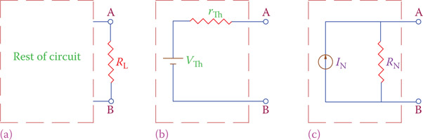
Figure 12.33
Comparison of Thevenin’s and Norton’s equivalent circuits. (a) Original circuit. (b) Thevenin’s circuit. (c) Norton’s circuit.

Figure 12.34
Norton equivalent of a circuit as seen from a load between points A and B. (a) Original circuit. (b) Norton’s equivalent circuit.
To find R,
- Disconnect RL (see Figure 12.34a).
- Replace each voltage source by its internal resistance.
- Remove any current source if it exists.
- Determine the resistance between A and B.
To find IN,
- Short RL (short circuit between A and B).
- Find the current flowing from A to B.
In fact, there is a correspondence between the values obtained for rTh, RN, and between VTH and IN. These are
| (12.12) |
| (12.13) |
Example 12.19
Find the Norton’s equivalent circuit for the circuit shown in Figure 12.28, as seen from the 32 Ω resistor. The internal resistances of the voltage sources are zero. The figure is repeated here for convenience.

Figure 12.28
Circuit of Example 12.19.

Figure 12.35
Norton’s Equivalent for the circuit in Figure 12.28.
Solution
The equivalent resistance RN is exactly found in the same way as in Example 12.16 and is not repeated here. Its value is 48 Ω.
The current from A to B when A and B are shorted together can be determined easier if the principle of superposition is used. First, the 6 V battery is removed. Because A is shorted to B the 120 Ω resistor does not receive any current and the current between A and B is 12 ÷ 80 = 0.15 A. Next, the 12 V battery is removed and the current between A and B is 6 ÷ 120 = 0.05 A. Thus, the total current is 0.15 + 0.05 = 0.20 A. The resultant Norton’s circuit is shown in Figure 12.35.
The current in the 32 Ω resistor is determined from considering that the total current shared between the 32 Ω resistor and RN (=48 Ω) is 0.2 A. This current is divided between them and based on their values ratio the smaller resistor take the higher current. Thus,
If instead of 32 Ω the value of this resistor changes to 64 Ω, for instance, the new value of the current is
Note that in finding IN, it would be easier for this and some problems to use the relationship in Equation 12.13, if we already have the value of VTh.
12.7 High Voltage Direct Current Transmission
For very long distance transmission of electricity, as we discussed in this chapter, AC electricity carrying conductors introduce inductive and capacitive reactance. These two can become a burden and cause limitations on transmission lines, particularly for underground and underwater lines, where the distance between cables is much smaller than the overhead lines. For this reason and in some cases for strategic reasons (e.g., maintaining an undisturbed supply of electricity to cities), transmission in the form of direct current has been considered and is practiced. Obviously, line voltage must be high to avoid large voltage drop as well as too much loss of energy in the line.
For high voltage direct current (HVDC) transmission, at the power side (sending end) the voltage of DC electricity must be raised to some high level (e.g., a few hundred thousand volts). After transmission to the destination, this voltage must be reduced to the distribution (and finally consumption) level. Because no direct use of transformers is possible, these operations are much more complicated and costly than the counterparts in AC electricity. There are advantages and disadvantages for HVDC transmission, but a major factor is the cost that makes it prohibitive in many cases, unless the cost can be justified. The total cost for HVDC can well reach 10× of the cost for the same power AC transmission. As for example, the cost of HVDC is in the order of $10 million per mile, whereas for AC line it is in the range of $1 million per mile.
Among the advantages is the lack of length limitations as mentioned above (no line induction and capacitance) and that the voltage at the receiving end is not affected by phase distortion, which is possible with AC lines. Also, networks with different frequencies can be interconnected.
Among the disadvantages is the fact that no branching is possible in between the two ends, unless another costly station for voltage conversion is provided. For AC transmission it is relatively very inexpensive to add a new substation and branch into or from an existing grid.
Presently, there are a number of HVDC lines in the United States and elsewhere. These are in cases where advantages overcome the disadvantages, or there is no alternative for HVDC.
12.8 Chapter Summary
- Energy is transmitted from the generation site to the consumption site before being distributed among the consumers.
- To reduce loss of energy and voltage drop in transmission lines, voltage is raised, so that for the same power the line current is smaller.
- Transmission and distribution voltages are standardized and are categorized to low, medium, high, extra high, and ultrahigh voltage.
- Most conductors for transmission lines today are made of stranded aluminum and reinforced by steel cables.
- A substation is where voltage is changed or where various lines meet. It is equipped with switches and breakers and protection devices.
- The important electrical parameters of transmission lines are their electrical resistance, inductance, and capacitance. By itself this is like a small load between the two ends of transmission lines.
- Resistance in a conductor depends on its thickness, length, and material. Inductance and capacitance depend on the thickness, wire spacing, and line length for all conductors in a transmission line.
- Ampacity is the current carrying capacity of a line. This depends on the resistance and the generated heat in the conductor as well as how this heat can be disposed of, thus on the ambient temperature.
- The same conductor has different ampacities under different conditions.
- Conductor sizes are standardized. Electrical wires are made of copper or aluminum. The electrical resistance and weight of standard wires are tabulated and can be directly embedded in calculations.
- An electrical grid or network consists of many interconnections of lines between various electric sources and electric loads.
- For analysis of currents and voltages in different sections of more complex networks, use can be made of a number of methods that allow reducing the networks to simpler circuits. These are Kirchhoff’s voltage and current laws, Thevenin’s theorem, Norton’s theorem, and the principle of superposition.
- HVDC transmission is an alternative method for long distance when AC transmission faces limitation, but the cost is considerably higher.
Review Questions
- What are the main reasons to raise voltage for electricity transmission?
- How does raising voltage affect the voltage drop in an electric line?
- What are the three parameters that influence the resistance of electric wires?
- How does raising voltage affect power consumed in transmission lines?
- What is a substation? Name some of the major equipment in a substation.
- Is 220 V considered a high voltage? What about 11,000 V?
- Why can’t the output of a power station be directly connected to a transmission line?
- Is there any difference between transmission and distribution lines? Describe.
- Is there any difference between transmission and power lines? Describe.
- What happens if one ignores the inductance and capacitance of transmission lines?
- Is the voltage the same at the two ends of a transmission line? Why or why not?
- Does the phase difference between current and voltage stay the same along a transmission line? Why or why not?
- If the length of a line doubles, does its resistance double, too? Why or why not?
- What is ampacity? What factors affect ampacity?
- If the ambient temperature changes from –10°C to +10°C, does ampacity go up or down?
- What is transposition in transmission lines? Why is it necessary?
- What are the two main parameters affecting the inductance of power lines?
- Why is grounding important? What is the main objective of grounding?
- Where does the electricity go when a ground current exist? Does it dissipate in the ground?
- What are the advantages of Thevenin’s theorem and Norton’s theorem?
- What does the Kirchhoff’s voltage law imply?
- What does the Kirchhoff’s current law imply?
- What does the principle of superposition imply?
- What does HVDC mean, and what is it?
Problems
- The diameter of a round copper wire is 0.7620 mm. What is the resistance of a piece of this wire 150 m long? The specific resistance of copper in metric system is 1.6779 × 10⁻⁸ Ω.m.
- If the area of a copper wire is 0.0285 mm2, what is the resistance of 1 km of this wire?
- If the specific resistance of a metal in imperial system is 265 Ω.CM/ft, find its specific resistance in the metric system?
- Tungsten has a specific resistance of 5.6 × 10⁻⁸ Ω.m at room temperature (20°C). Find its specific resistance at 1800°C. Find the corresponding information from Table 12.2.
- What is the resistance of a tungsten wire with a cross-section area of 1 mm2 and 1 m long at 1000°C?
- Using numbers in Table 12.2 determine if the resistance of a copper wire 20 m long is more or an aluminum wire 15 m long if both have the same cross-section area.
- What length of a tungsten filament of a lightbulb with a 0.05 mm diameter is required for 10 Ω resistance at 20°C temperature?
- The resistance of a piece of wire 1000 ft long is 2 Ω. If the wire is made out of copper, find its diameter in inches.
- For the wire in Problem 8 find the thickness in CM (circular mil).
- The diameter of a piece of round tungsten wire is 32 mils. What length of this metal makes a resistance of 20 Ω?
- If the resistance of a length of aluminum wire at 20°C is 2 Ω, what is its resistance at 100°C? Use the information in Table 12.2.
- From Table 12.4 find the allowable current in a TW type copper wire gauge AWG-12 for free air installation in an ambient reaching 100°F. The voltage is below 2000 V.
- For the wire in Problem 12 find the resistance and the weight for 5 km of this wire.
- If the wire in Problem 12 must be used in a conduit, what is the ampacity under the same ambient conditions?
- Determine the wire gauge for 60 A current in a conduit where two of such copper wires are to be installed. The ambient temperature does not go over 25°C. The operating voltage is below 2000 V and the wire type is TW.
- For a pair of single-phase lines, 3 ft apart gauge 2 wire is used. Find the inductance of 500 m of this line? Use Table 12.4 for the required information.
- If the line in Problem 16 carries 60 Hz electricity, what is its inductive reactance per mile?
- If the wire in Problem 16 is used for transmission of three-phase 60 Hz electricity and the conductors are completely transposed, find the inductance per mile if the three lines are on the corners of a triangle and 3 ft apart from each other.
- Three cables of 40 mm diameter are used in a transmission line arranged as shown in Figure 12.16b. The distances between the lines, are 3, 3, and 6 m, respectively. Find the inductance of the line per phase and the inductive reactance for a completely transposed line 100 km long for 50 Hz.
- A six conductor transmission line uses 2 in diameter aluminum cables. The lines are arranged in two rows each consisting of three cables as shown in Figure 12.16b. If the vertical distance between each pair of adjacent wires is 10 ft and the horizontal distance for the adjacent pairs is 15 ft, find the unit inductance of the line per phase. The line is completely transposed.
- If the line in Problem 20 is 20 mi (32.18 km) long, what is its inductance per phase?
- If the wire in Problem 20 has 0.1563 Ω resistance per mile, what is its impedance per mile per phase, ignoring the capacitance? The line frequency is 60 Hz.
- Find the capacitance per mile for the line in Problem 18.
- Find the capacitive reactance per mile for the line in Problem 18.
- Find the impedance per mile for line in Problem 18 if the ohmic resistance per mile is 0.3 Ω.
- Determine the capacitance for the transmission line in Problem 20.
- Find the current change in resistor RL in the circuit of Figure P12.1 when RL changes between 51 Ω ± 20%.

Figure P12.1 Circuit for Problem 27.
- Repeat Problem 27 using Thevenin’s theorem (find the Thevenin’s equivalent circuit as seen from the 51 Ω resistor). Assume the internal resistances of the power supplies to be zero.
- Modify the circuit in Figure P12.2 to its simplest form that you can.
-

Figure P12.2 Circuit for Problem 29.
For the circuit shown in Figure P12.3, find the equivalent Thevenin’s circuit as seen from the 500 Ω resistor.
Figure P12.3 Circuit for Problem 30.
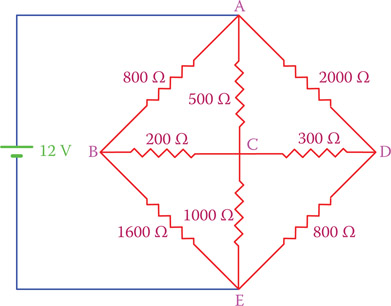
Figure P12.4 Circuit for Problem 32.
- Find the Norton’s equivalent circuit for the circuit of Problem 30.
- Find the current in each resistance in the circuit as shown in Figure P12.4 by eploying Kirchoff’s laws.
Advanced Learning: Positive, Negative, and Zero Sequence for Fault Analysis
When a fault occurs in part of a line, it must be detected and acted upon. Detection is performed by some sort of sensor, measuring current, voltage, etc. Selection of sensors with correct and proper rating and able to act correctly without getting damaged is important. This section is added so that an advanced reader becomes familiar with three important terms that are used for the analysis of fault situations.
Because various faults can occur in an electric network and at different places (e.g., at a generator site, a load site, a transformer, and any point of a transmission line), each fault must be detected and the proper action be taken. A fault introduces a large disturbance in a network and causes a large imbalance in the system. Even if a system has an unbalanced load prior to a fault, the imbalance situation caused by a fault dominates the normal operating condition.
Thus, detection of a fault starts with an analysis of the unbalanced loads. The terms positive sequence, negative sequence, and zero sequence are used to define the imbalance condition in an electric network. The full discussion is out of the scope of this book. So we confine this section to only the definitions.
So far, we have considered any three-phase system to consist of three voltages and the corresponding currents with 120° phase difference between them. In a more general scope, any such system can be considered to consist of those three components (which constitute the positive sequence components) and six other components. The above three components rotate in a positive direction. Three similar components rotating in the opposite direction are called negative sequence components, and finally another set of similar components that do not rotate are called zero sequence components. The advantage of this expansion is that an unbalanced system can be expressed in terms of three sets of three balanced systems, which are its positive, negative, and zero sequence components.
Positive sequence: One of three balanced components of any unbalanced condition in a three-phase system. The positive sequence comprises three vectors with a positive sense of direction of rotation. Balanced components are used for detection of faults, particularly ground faults, in three-phase generators, loads and transformers (see also negative sequence).
Negative sequence: One of three sets of balanced components (represented by equal size vectors, 120° apart from each other) of any unbalanced condition in a three-phase system. The imbalance condition is more noticeable when a fault happens. Thus, decomposition to balanced components is used for detection of faults in three-phase generators, loads, and transformers. The sense of direction for negative sequence is negative, as opposed to the direction for positive sequence.
Zero sequence: One of the three balanced components when any unbalanced condition (or load) in a three-phase system can be decomposed into balanced components. The zero sequence comprises three equal vectors that together with positive sequence and negative sequence vectors can represent the unbalanced condition. See also the positive sequence and negative sequence.
Figure A12.1a shows three vectors A, B, and C. They can represent three unbalanced voltages or three unbalanced currents in a three-phase electric circuit. Associated with their values, three sets of vectors that are shown in Figure A12.1b can be found. These vectors are specific to the vector conditions in Figure A12.1a. They are the zero (a0, b0, and c0), negative (a2, b2, and c2), and positive (a1, b1, and c1) components, respectively, for A, B, and C. Figure A12.1c shows the composition of each vector (A, B, and C) of the components from the three sequence sets depicted in Figure A12.1b. That is,
A = a0 + a1 + a2 B = b0 + b1 + b2 C = c0 + c1 + c2
Note that the vectors making the positive sequence components and the negative sequence components are at 120° from each other, whereas the zero sequence components are at 0° from each other.
Not necessarily all the components must have nonzero values. For instance, in a generator delivering electricity to a balanced load, only the positive sequence values exist and the others are zero. The nonzero components obtain values if the load is unbalanced or a fault occurs.
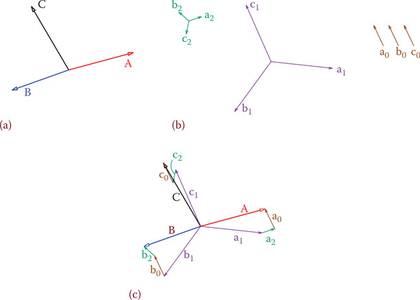
Figure A12.1Decomposition of an unbalanced condition to three sets of balanced components. (a) Three vectors of currents in a three-phase system. (b) Three sets of vectors representing positive (a1, b1, c1), negative (a2, b2, c2) and zero (a0, b0, c0) sequences. (c) Result of decomposition to sequence components.
The zero sequence components are very helpful in dealing with ground faults. The values of zero sequence components for various faults for any device, such as a generator or a setup like a transformer with delta-delta connection, are analyzed and determined. The results can be used for the deployment of the appropriate relaying (sensing) and protective devices.
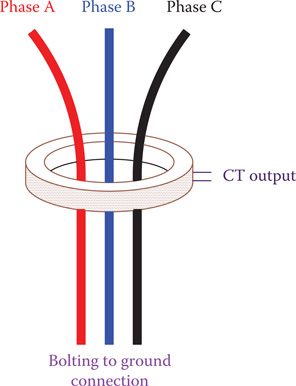
Figure A12.2
Current transformer for ground fault detection.
For detection of ground faults a current transformer (CT) is used. The three lines in a Y connection pass through the winding of a current transformer before being connected together and to the ground, as shown in Figure A12.2. The currents in the three lines add up together in this way and are measured by the current transformer. This is, in fact, the neutral current. In the normal conditions, particularly for balanced loads the current measured this way is zero, because the three currents in the three lines are 120° out of phase. When a ground fault occurs, the neutral current is not zero anymore. A high current in the neutral causes a voltage in the CT winding. This current can be high and a CT must be rated for it.