
Binary Space Partitioning Trees*
Bruce F. Naylor†
University of Texas, Austin
21.2BSP Trees as a Multi-Dimensional Search Structure
Total Ordering of a Collection of Objects•Visibility Ordering as Tree Traversal•Intra-Object Visibility
21.4BSP Tree as a Hierarchy of Regions
Tree Merging•Good BSP Trees• Converting B-Reps to Trees• Boundary Representations vs. BSP Trees
In most applications involving computation with 3D geometric models, manipulating objects and generating images of objects are crucial operations. Performing these operations requires determining for every frame of an animation the spatial relations between objects: how they might intersect each other, and how they may occlude each other. However, the objects, rather than being monolithic, are most often comprised of many pieces, such as by many polygons forming the faces of polyhedra. The number of pieces may be anywhere from the 100’s to the 1,000,000’s. To compute spatial relations between n polygons by brute force entails comparing every pair of polygons, and so would require O(n2). For large scenes comprised of 105 polygons, this would mean 1010 operations, which is much more than necessary.
The number of operations can be substantially reduced to anywhere from O(n log2n) when the objects interpenetrate (and so in our example reduced to 106), to as little as constant time, O(1), when they are somewhat separated from each other. This can be accomplished by using Binary Space Partitioning Trees, also called BSP Trees. They provide a computational representation of space that simultaneously provides a search structure and a representation of geometry. The reduction in number of operations occurs because BSP Trees provide a kind of “spatial sorting.” In fact, they are a generalization to dimensions > 1 of binary search trees, which have been widely used for representing sorted lists. Figure 21.1 below gives an introductory example showing how a binary tree of lines, instead of points, can be used to “sort” four geometric objects, as opposed to sorting symbolic objects such as names.
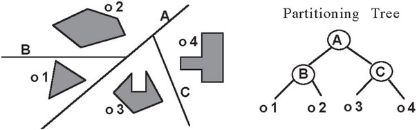
Figure 21.1BSP Tree representation of inter-object spatial relations.
Constructing a BSP Tree representation of one or more polyhedral objects involves computing the spatial relations between polygonal faces once and encoding these relations in a binary tree (Figure 21.2). This tree can then be transformed and merged with other trees to very quickly compute the spatial relations (for visibility and intersections) between the polygons of two moving objects.
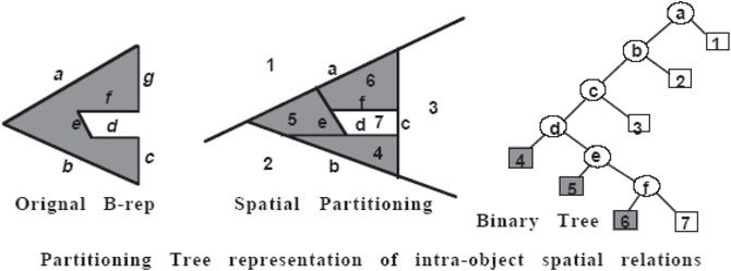
Figure 21.2Partitioning Tree representation of intra-object spatial relations.
As long as the relations encoded by a tree remain valid, which for a rigid body is forever, one can reap the benefits of having generated this tree structure every time the tree is used in subsequent operations. The return on investment manifests itself as substantially faster algorithms for computing intersections and visibility orderings. And for animation and interactive applications, these savings can accrue over hundreds of thousands of frames. BSP Trees achieve an elegant solution to a number of important problems in geometric computation by exploiting two very simple properties occurring whenever a single plane separates (lies between) two or more objects: (1) any object on one side of the plane cannot intersect any object on the other side, (2) given a viewing position, objects on the same side as the viewer can have their images drawn on top of the images of objects on the opposite side (Painter’s Algorithm). See Figure 21.3.
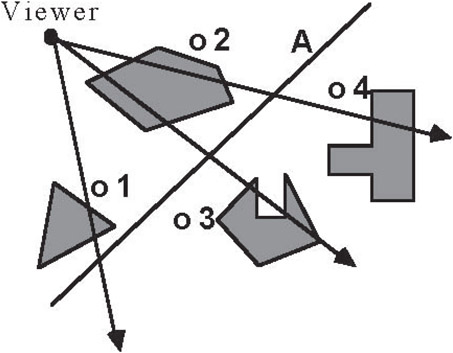
Figure 21.3Plane power: sorting objects w.r.t a hyperplane.
These properties can be made dimension independent if we use the term “hyperplane” to refer to planes in 3D, lines in 2D, and in general for d-space, to a (d − 1)-dimensional subspace defined by a single linear equation. The only operation we will need for constructing BSP Trees is the partitioning of a convex region by a singe hyperplane into two child regions, both of which are also convex as a result (Figure 21.4).
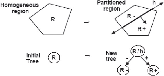
Figure 21.4Elementary operation used to construct BSP Trees.
BSP Trees exploit the properties of separating planes by using one very simple but powerful technique to represent any object or collection of objects: recursive subdivision by hyperplanes. A BSP Tree is the recording of this process of recursive subdivision in the form of a binary tree of hyperplanes. Since there is no restriction on what hyperplanes are used, polytopes (polyhedra, polygons, etc.) can be represented exactly. A BSP Tree is a program for performing intersections between the hyperplane’s halfspaces and any other geometric entity. Since subdivision generates increasingly smaller regions of space, the order of the hyperplanes is chosen so that following a path deeper into the tree corresponds to adding more detail, yielding a multi-resolution representation. This leads to efficient intersection computations. To determine visibility, all that is required is choosing at each tree node which of the two branches to draw first based solely on which branch contains the viewer. No other single representation of geometry inherently answers questions of intersection and visibility for a scene of 3D moving objects. And this is accomplished in a computationally efficient and parallelizable manner.
21.2BSP Trees as a Multi-Dimensional Search Structure
Spatial search structures are based on the same ideas that were developed in Computer Science during the 60’s and 70’s to solve the problem of quickly processing large sets of symbolic data, as opposed to geometric data, such as lists of people’s names. It was discovered that by first sorting a list of names alphabetically, and storing the sorted list in an array, one can find out whether some new name is already in the list in log2n operations using a binary search algorithm, instead of n/2 expected operations required by a sequential search. This is a good example of extracting structure (alphabetical order) existing in the list of names and exploiting that structure in subsequent operations (looking up a name) to reduce computation. However, if one wishes to permit additions and deletions of names while maintaining a sorted list, then a dynamic data structure is needed, that is, one using pointers. One of the most common examples of such a data structure is the binary search tree.
A binary search tree (See also Chapter 3) is illustrated in Figure 21.5, where it is being used to represent a set of integers S = {0, 1, 4, 5, 6, 8} lying on the real line. We have included both the binary tree and the hierarchy of intervals represented by this tree. To find out whether a number/point is already in the tree, one inserts the point into the tree and follows the path corresponding to the sequence of nested intervals that contain the point. For a balanced tree, this process will take no more than O( log n) steps; for in fact, we have performed a binary search, but one using a tree instead of an array. Indeed, the tree itself encodes a portion of the search algorithm since it prescribes the order in which the search proceeds.
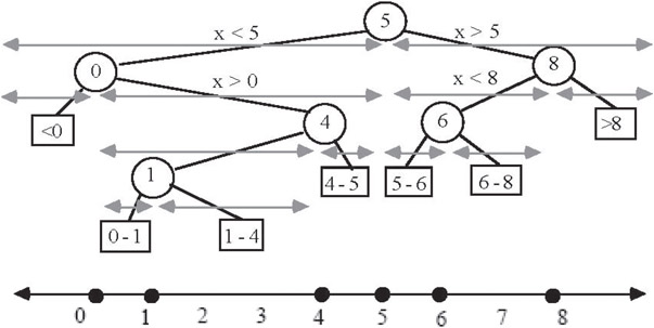
Figure 21.5A binary search tree.
This now brings us back to BSP Trees, for as we said earlier, they are a generalization of binary search trees to dimensions > 1 (in 1D, they are essentially identical). In fact, constructing a BSP Tree can be thought of as a geometric version of Quick Sort. Modifications (insertions and deletions) are achieved by merging trees, analogous to merging sorted lists in Merge Sort. However, since points do not divide space for any dimension > 1, we must use hyperplanes instead of points by which to subdivide. Hyperplanes always partition a region into two halfspaces regardless of the dimension. In 1D, they look like points since they are also 0D sets; the one difference being the addition of a normal denoting the “greater than” side. In Figure 21.6, we show a restricted variety of BSP Trees that most clearly illustrates the generalization of binary search trees to higher dimensions. (You may want to call this a k-d tree, but the standard semantics of k-d trees does not include representing continuous sets of points, but rather finite sets of points.) BSP Trees are also a geometric variety of Decision Trees, which are commonly used for classification (e.g., biological taxonomies), and are widely used in machine learning. Decision trees have also been used for proving lower bounds, the most famous showing that sorting is Ω(n log n). They are also the model of the popular “20 questions” game (I’m thinking of something and you have 20 yes/no question to guess what it is). For BSP Trees, the questions become “what side of a particular hyperplane does some piece of geometry lie.”
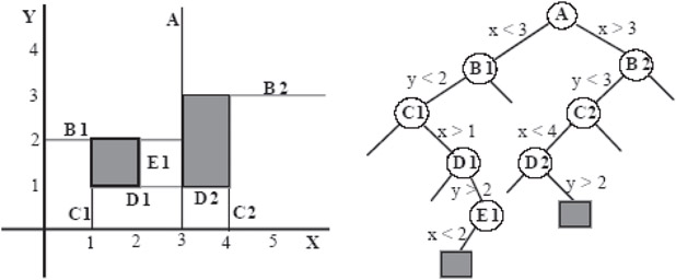
Figure 21.6Extension of binary search trees to 2D as a BSP Tree.
Visibility orderings are used in image synthesis for visible surface determination (hidden surface removal), shadow computations, ray tracing, beam tracing, and radiosity. For a given center of projection, such as the position of a viewer or of a light source, they provide an ordering of geometric entities, such as objects or faces of objects, consistent with the order in which any ray originating at the center might intersect the entities. Loosely speaking, a visibility ordering assigns a priority to each object or face so that closer objects have priority over objects further away. Any ray emanating from the center or projection that intersects two objects or faces, will always intersect the surface with higher priority first. The simplest use of visibility orderings is with the “Painter’s Algorithm” for solving the hidden surface problem. Faces are drawn into a frame-buffer in far-to-near order (low-to-high priority), so that the image of nearer objects/polygons over-writes those of more distant ones.
A visibility ordering can be generated using a single hyperplane; however, each geometric entity or “object” (polyhedron, polygon, line, point) must lie completely on one side of the hyperplane, that is, no objects are allowed to cross the hyperplane. This requirement can always be induced by partitioning objects by the desired hyperplane into two “halves”. The objects on the side containing the viewer are said to have visibility priority over objects on the opposite side; that is, any ray emanating from the viewer that intersects two objects on opposite sides of the hyperplane will always intersect the near side object before it intersects the far side object. See Figures 21.7 and 21.8.

Figure 21.7Left side has priority over right side.
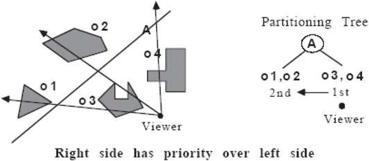
Figure 21.8Right side has priority over left side.
21.3.1Total Ordering of a Collection of Objects
A single hyperplane cannot order objects lying on the same side, and so cannot provide a total visibility ordering. Consequently, in order to exploit this idea, we must extend it somehow so that a visibility ordering for the entire set of objects can be generated. One way to do this would be to create a unique separating hyperplane for every pair of objects. However, for n objects this would require n2 hyperplanes, which is too many.
The required number of separating hyperplanes can be reduced to as little as n by using the geometric version of recursive subdivision (divide and conquer). If the subdivision is performed using hyperplanes whose position and orientation is unrestricted, then the result is a BSP Tree. The objects are first separated into two groups by some appropriately chosen hyperplane (Figure 21.9). Then each of the two groups is independently partitioned into two sub-groups (for a total now of 4 sub-groups). The recursive subdivision continues in a similar fashion until each object, or piece of an object, is in a separate cell of the partitioning. This process of partitioning space by hyperplanes is naturally represented as a binary tree (Figure 21.10).
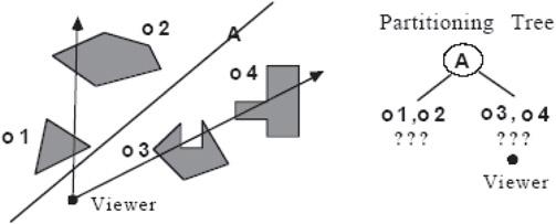
Figure 21.9Separating objects with a hyperplane.
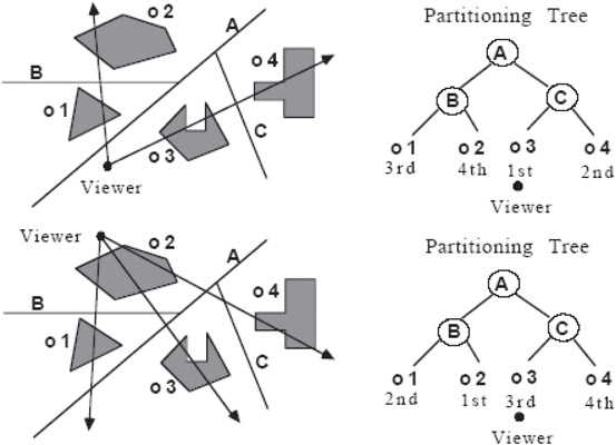
Figure 21.10Binary tree representation of space partitioning.
21.3.2Visibility Ordering as Tree Traversal
How can this tree be used to generate a visibility ordering on the collection of objects? For any given viewing position, we first determine on which side of the root hyperplane the viewer lies. From this we know that all objects in the near-side subtree have higher priority than all objects in the far-side subtree; and we have made this determination with only a constant amount of computation (in fact, only a dot product). We now need to order the near-side objects, followed by an ordering of the far-side objects. Since we have a recursively defined structure, any subtree has the same form computationally as the whole tree. Therefore, we simply apply this technique for ordering subtrees recursively, going left or right first at each node, depending upon which side of the node’s hyperplane the viewer lies. This results in a traversal of the entire tree, in near-to-far order, using only O(n) operations, which is optimal (this analysis is correct only if no objects have been split; otherwise it is > n).
The schema we have just described is only for inter-object visibility, that is, between individual objects. And only when the objects are both convex and separable by a hyperplane is the schema a complete method for determining visibility. To address the general unrestricted case, we need to solve intra-object visibility, that is, correctly ordering the faces of a single object. BSP Trees can solve this problem as well. To accomplish this, we need to change our focus from convex cells containing objects to the idea of hyperplanes containing faces. Let us return to the analysis of visibility with respect to a hyperplane. If instead of ordering objects, we wish to order faces, we can exploit the fact that not only can faces lie on each side of a hyperplane as objects do, but they can also lie on the hyperplane itself. This gives us a 3-way ordering of: near → on → far (Figure 21.11).
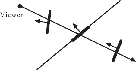
Figure 21.11Ordering of polygons: near → on → far.
If we choose hyperplanes by which to partition space that always contain a face of an object, then we can build a BSP Tree by applying this schema recursively as before, until every face lies in some partitioning hyperplane contained in the tree. To generate a visibility ordering of the faces in this intra-object tree, we use the method above with one extension: faces lying on hyperplanes are included in the ordering, that is, at each node, we generate the visibility ordering of near-subtree → on-faces → far-subtree. Using visibility orderings provides an alternative to z-buffer based algorithms. They obviate the need for computing and comparing z-values, which is very susceptible to numerical error because of the perspective projection. In addition, they eliminate the need for z-buffer memory itself, which can be substantial (80 Mbytes) if used at a sub-pixel resolution of 4×4 to provide anti-aliasing. More importantly, visibility orderings permit unlimited use of transparency (non-refractive) with no additional computational effort, since the visibility ordering gives the correct order for compositing faces using alpha blending. And in addition, if a near-to-far ordering is used, then rendering completely occluded objects/faces can be eliminated, such as when a wall occludes the rest of a building, using a beam-tracing based algorithm.
21.4BSP Tree as a Hierarchy of Regions
Another way to look at BSP Trees is to focus on the hierarchy of regions created by the recursive partitioning, instead of focusing on the hyperplanes themselves. This view helps us to see more easily how intersections are efficiently computed. The key idea is to think of a BSP Tree region as serving as a bounding volume: each node v corresponds to a convex volume that completely contains all the geometry represented by the subtree rooted at v. Therefore, if some other geometric entity, such as a point, ray, object, etc., is found to not intersect the bounding volume, then no intersection computations need be performed with any geometry within that volume.
Consider as an example a situation in which we are given some test point and we want to find which object if any this point lies in. Initially, we know only that the point lies somewhere space (Figure 21.12).
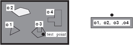
Figure 21.12Point can lie anywhere.
By comparing the location of the point with respect to the first partitioning hyperplane, we can find in which of the two regions (a.k.a. bounding volumes) the point lies. This eliminates half of the objects (Figure 21.13).

Figure 21.13Point must lie to the right of the hyperplane.
By continuing this process recursively, we are in effect using the regions as a hierarchy of bounding volumes, each bounding volume being a rough approximation of the geometry it bounds, to quickly narrow our search (Figure 21.14).
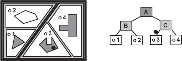
Figure 21.14Point’s location is narrowed down to one object.
For a BSP Tree of a single object, this region-based (volumetric) view reveals how BSP Trees can provide a multi-resolution representation. As one descends a path of the tree, the regions decrease in size monotonically. For curved objects, the regions converge in the limit to the curve/surface. Truncating the tree produces an approximation, ala the Taylor series of approximations for functions (Figure 21.15).
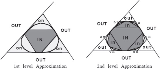
Figure 21.15Multiresolution representation provided by BSP tree.
The spatial relations between two objects, each represented by a separate tree, can be determined efficiently by merging two trees. This is a fundamental operation that can be used to solve a number of geometric problems. These include set operations for CSG modeling as well as collision detection for dynamics. For rendering, merging all object-trees into a single model-tree determines inter-object visibility orderings; and the model-tree can be intersected with the view-volume to efficiently cull away off-screen portions of the scene and provide solid cutaways with the near clipping plane. In the case where objects are both transparent and interpenetrate, tree merging acts as a view independent geometric sorting of the object faces; each tree is used in a manner analogous to the way Merge Sort merges previously sorted lists to quickly created a new sorted list (in our case, a new tree). The model-tree can be rendered using ray tracing, radiosity, or polygon drawing using a far-to-near ordering with alpha blending for transparency. An even better alternative is multi-resolution beam-tracing, since entire occluded subtrees can be eliminated without visiting the contents of the subtree, and distance subtrees can be pruned to the desired resolution. Beam tracing can also be used to efficiently compute shadows.
All of this requires as a basic operation an algorithm for merging two trees. Tree merging is a recursive process, which proceeds down the trees in a multi-resolution fashion, going from low-res to high-res. It is easiest to understand in terms of merging a hierarchy of bounding volumes. As the process proceeds, pairs of tree regions, a.k.a. convex bounding volumes, one from each tree, are compared to determine whether they intersect or not. If they do not, the contents of the corresponding subtrees are never compared. This has the effect of “zooming in” on those regions of space where the surfaces of the two objects intersect (Figure 21.16).
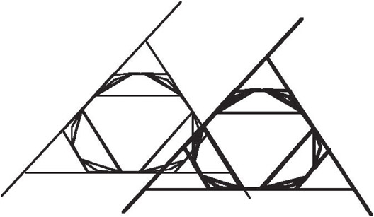
Figure 21.16Merging BSP Trees.
The algorithm for tree merging is quite simple once you have a routine for partitioning a tree by a hyperplane into two trees. The process can be thought of in terms of inserting one tree into the other in a recursive manner. Given trees T1 and T2, at each node of T1 the hyperplane at that node is used to partition T2 into two “halves”. Then each half is merged with the subtree of T1 lying on the same side of the hyperplane. (In actuality, the algorithm is symmetric w.r.t. the role of T1 and T2 so that at each recursive call, T1 can split T2 or T2 can split T1.)
 Merge_Bspts : ( T1, T2 : Bspt ) -> Bspt
    Types
       BinaryPartitioner : { hyperplane, sub-hyperplane}
       PartitionedBspt : ( inNegHs, inPosHs : Bspt )

    Imports
       Merge_Tree_With_Cell : ( T1, T2 : Bspt ) -> Bspt User defined semantics.
       Partition_Bspt : ( Bspt, BinaryPartitioner ) -> PartitionedBspt

    Definition
       IF T1.is_a_cell OR T2.is_a_cell
       THEN
         VAL := Merge_Tree_With_Cell( T1, T2 )
       ELSE
         Partition_Bspt( T2, T1.binary_partitioner ) -> T2_partitioned
         VAL.neg_subtree := Merge_Bspts(T1.neg_subtree, T2_partitioned.inNegHs)
         VAL.pos_subtree:= Merge_Bspts(T1.pos_subtree, T2_partitioned.inPosHs )
       END
    RETURN} VAL
    END Merge_Bspts
While tree merging is easiest to understand in terms of comparing bounding volumes, the actual mechanism uses sub-hyperplanes, which is more efficient. A sub-hyperplane is created whenever a region is partitioned by a hyperplane, and it is just the subset of the hyperplane lying within that region. In fact, all of the illustrations of trees we have used are drawings of sub-hyperplanes. In 3D, these are convex polygons, and they separate the two child regions of an internal node. Tree merging uses sub-hyperplanes to simultaneously determine the spatial relations of four regions, two from each tree, by comparing the two sub-hyperplanes at the root of each tree. For 3D, this is computed using two applications of convex-polygon clipping to a plane, and there are three possible outcomes: intersecting, non-intersecting and coincident (Figure 21.17). This is the only overtly geometric computation in tree merging; everything else is data structure manipulation.
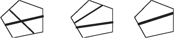
Figure 21.17Three cases (intersecting, non-intersecting, coincident) when comparing sub-hyperplanes during tree merging.
For any given set, there exist an arbitrary number of different BSP Trees that can represent that set. This is analogous to there being many different programs for computing the same function, since a BSP Tree may in fact be interpreted as a computation graph specifying a particular search of space. Similarly, not all programs/algorithms are equally efficient, and not all searches/trees are equally efficient. Thus the question arises as to what constitutes a good BSP Tree. The answer is a tree that represents the set as a sequence of approximations. This provides a multi-resolution representation. By pruning the tree at various depths, different approximations of the set can be created. Each pruned subtree is replaced with a cell containing a low degree polynomial approximation of the set represented by the subtree (Figures 21.18 and 21.19).
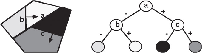
Figure 21.18Before pruning.
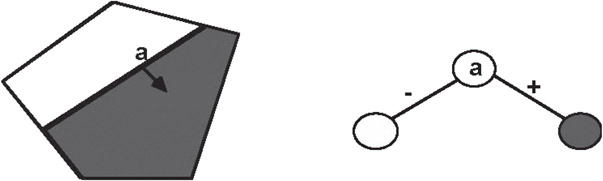
Figure 21.19After pruning.
In Figure 21.20, we show two quite different ways to represent a convex polygon, only the second of which employs the sequence of approximations idea. The tree on the left subdivides space using lines radiating from the polygonal center, splitting the number of faces in half at each step of the recursive subdivision. The hyperplanes containing the polygonal edges are chosen only when the number of faces equals one, and so are last along any path. If the number of polygonal edges is n, then the tree is of size O(n) and of depth O( log n). In contrast, the tree on the right uses the idea of a sequence of approximations. The first three partitioning hyperplanes form a first approximation to the exterior while the next three form a first approximation to the interior. This divides the set of edges into three sets. For each of these, we choose the hyperplane of the middle face by which to partition, and by doing so refine our representation of the exterior. Two additional hyperplanes refine the interior and divide the remaining set of edges into two nearly equal sized sets. This process precedes recursively until all edges are in partitioning hyperplanes. Now, this tree is also of size O(n) and depth O( log n), and thus the worst case, say for point classification, is the same for both trees. Yet they appear to be quite different.
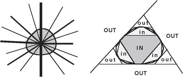
Figure 21.20Illustration of bad vs. good trees.
This apparent qualitative difference can be made quantitative by, for example, considering the expected case for point classification. With the first tree, all cells are at depth log n, so the expected case is the same as the worst case regardless of the sample space from which a point is chosen. However, with the second tree, the top three out-cells would typically constitute most of the sample space, and so a point would often be classified as OUT by, on average, two point-hyperplane tests. Thus the expected case would converge to O(1) as the ratio of polygon-area/sample-area approaches 0. For line classification, the two trees differ not only in the expected case but also in the worst case: O(n) vs. O( log n). For merging two trees the difference is O(n2) vs. O(n log n). This reduces even further to O( log n) when the objects are only contacting each other, rather overlapping, as is the case for collision detection. However, there are worst case “basket weaving” examples that do require O(n2) operations. These are geometric versions of the Cartesian product, as for example when a checkerboard is constructed from n horizontal strips and n vertical strips to produce n × n squares. These examples, however, violate the Principle of Locality: that geometric features are local not global features. For almost all geometric models of physical objects, the geometric features are local features. Spatial partitioning schemes can accelerate computations only when the features are in fact local, otherwise there is no significant subset of space that can be eliminated from consideration. The key to a quantitative evaluation, and also generation, of BSP Trees is to use expected case models, instead of worst-case analysis. Good trees are ones that have low expected cost for the operations and distributions of input of interest. This means, roughly, that high probability regions can be reached with low cost, that is, they have short paths from the root to the corresponding node, and similarly low probability regions should have longer paths. This is exactly the same idea used in Huffman codes. For geometric computation, the probability of some geometric entity, such as a point, line segment, plane, etc., lying in some arbitrary region is typically correlated positively to the size of the region: the larger the region the greater the probability that a randomly chosen geometric entity will intersect that region. To compute the expected cost of a particular operation for a given tree, we need to know at each branch in the tree the probability of taking the left branch, p, and the probability of taking the right branch p+. If we assign a unit cost to the partitioning operation, then we can compute the expected cost exactly, given the branch probabilities, using the following recurrence relation:
Ecost[T]=
   IF T is a cell
   THEN 0
   ELSE 1 + p− ∗ Ecost[T−] + p+ ∗ Ecost[T+]
This formula does not directly express any dependency upon a particular operation; those characteristics are encoded in the two probabilities p− and p+. Once a model for these is specified, the expected cost for a particular operation can be computed for any tree.
As an example, consider point classification in which a random point is chosen from a uniform distribution over some initial region R. For a tree region of r with child regions r+ and r−, we need the conditional probability of the point lying in r+ and r−, given that it lies in r. For a uniform distribution, this is determined by the sizes of the two child-regions relative to their parent:
Similar models have been developed for line, ray and plane classification. Below we describe how to use these to build good trees.
21.4.3Converting B-Reps to Trees
Since humans do not see physical objects in terms of binary trees, it is important to know how such a tree be constructed from something that is more intuitive. The most common method is to convert a boundary representation, which corresponds more closely to how humans see the world, into a tree. In order for a BSP Tree to represent a solid object, each cell of the tree must be classified as being either entirely inside or outside of the object; thus, each leaf node corresponds to either an in-cell or an out-cell. The boundary of the set then lies between in-cells and out-cells; and since the cells are bounded by the partitioning hyperplanes, it is necessary for the entire boundary to lie in the partitioning hyperplanes (Figure 21.21).
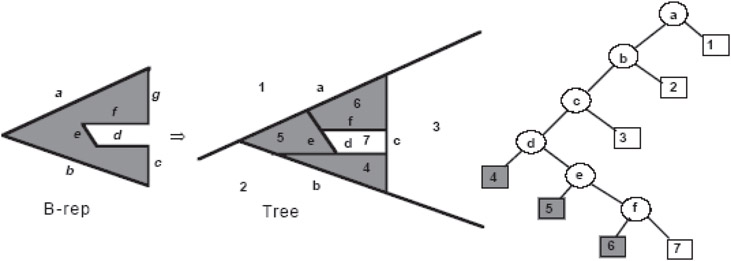
Figure 21.21B-rep and Tree representation of a polygon.
Therefore, we can convert from a b-rep to a tree simply by using all of the face hyperplanes as partitioning hyperplanes. The face hyperplanes can be chosen in any order and the resulting tree will always generate a convex decomposition of the interior and the exterior. If the hyperplane normals of the b-rep faces are consistently oriented to point to the exterior, then all left leaves will be in-cells and all right leaves will be out-cells. The following algorithm summarizes the process.
Brep_to_Bspt: Brep b − > Bspt T
IF b == NULL
THEN
 T = if a left-leaf then an in-cell else an out-cell
ELSE
 h = Choose_Hyperplane(b)
 {b+, b−, b0} = Partition_Brep(b,h)
 T.faces = b0
 T.pos_subtree = Brep_to_Bspt(b+)
 T.neg_subtree = Brep_to_Bspt(b−)
END
However, this does not tell us in what order to choose the hyperplanes so as to produce the best trees. Since the only known method for finding the optimal tree is by exhaustive enumeration, and there are at least n! trees given n unique face hyperplanes, we must employ heuristics. In 3D, we use both the face planes as candidate partitioning hyperplanes, as well as planes that go through face vertices and have predetermined directions, such as aligned with the coordinates axes. Given any candidate hyperplane, we can try to predict how effective it will be using expected case models; that is, we can estimate the expected cost of a subtree should we choose this candidate to be at its root. We will then choose the least cost candidate. Given a region r containing boundary b which we are going to partition by a candidate h, we can compute exactly p+ and p− for a given operation, as well as the size of b+ and b−. However, we can only estimate Ecost[T+] and Ecost[T−]. The estimators for these values can depend only upon a few simple properties such as number of faces in each halfspace, how many faces would be split by this hyperplane, and how many faces lie on the hyperplane (or area of such faces). Currently, we use |b+ |n for Ecost[T+], where n typically varies between .8 and .95, and similarly for Ecost[T−]. We also include a small penalty for splitting a face by increasing its contribution to b+ and b− from 1.0 to somewhere between 1.25 and 1.75, depending upon the object. We also favor candidates containing larger surface area, both in our heuristic evaluation and by first sorting the faces by surface area and considering only the planes of the top k faces as candidates. One interesting consequence of using expected case models is that choosing the candidate that attempts to balance the tree is usually not the best; instead the model prefers candidates that place small amounts of geometry in large regions, since this will result in high probability and low cost subtrees, and similarly large amounts of geometry in small regions. Balanced is optimal only when the geometry is uniformly distributed, which is rarely the case (Figure 21.22). More importantly, minimizing expected costs produces trees that represents the object as a sequence of approximations, and so in a multi-resolution fashion.
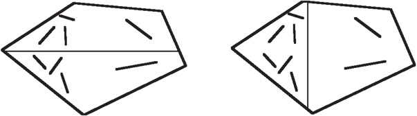
Figure 21.22Balanced is not optimal for non-uniform distributions.
21.4.4Boundary Representations vs. BSP Trees
Boundary Representations and BSP Trees may be viewed as complementary representations expressing difference aspects of geometry, the former being topological, the later expressing hierarchical set membership. B-reps are well suited for interactive specification of geometry, expressing topological deformations, and scan-conversion. BSP Trees are well suited for intersection and visibility calculations. Their relationship is probably more akin to the capacitor vs. inductor, than the tube vs. transistor.
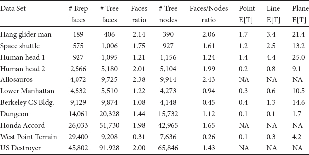
The most often asked question is what is the size of a BSP Tree representation of a polyhedron vs. the size of its boundary representation. This, of course, ignores the fact that expected cost, measured over the suite of operations for which the representation will be used, is the appropriate metric. Also, boundary representations must be supplemented by other devices, such as octrees, bounding volumes hierarchies, and z-buffers, in order to achieve an efficient system; and so the cost of creating and maintaining these structure should be brought into the equation. However, given the intrinsic methodological difficulties in performing a compelling empirical comparison, we will close with a few examples giving the original number of b-rep faces and the resulting tree using our currently implemented tree construction machinery. The first ratio is number-of-tree-faces/number-of-brep-faces. The second ratio is number-of-tree-nodes/number-of-brep-faces, where number-of-tree-nodes is the number of internal nodes. The last column is the expected cost in terms of point, line and plane classification, respectively, in percentage of the total number of internal nodes, and where the sample space was a bounding box 1.1 times the minimum axis-aligned bounding box. These numbers are pessimistic since typical sample spaces would be much larger than an object’s bounding box. Also, the heuristics are controlled by 4 parameters, and these numbers were generated, with some exceptions, without a search of the parameter space but rather using default parameters. There are also quite a number of ways to improve the conversion process, so it should be possible to do even better.
1.S.H. Bloomberg, A Representation of Solid Objects for Performing Boolean Operations, U.N.C. Computer Science Technical Report 86–006 1986.
2.W. Thibault and B. Naylor, Set operations on polyhedra using binary space BSP Trees, Computer Graphics, Vol. 21(4), pp. 153–162, July 1987.
3.B. F. Naylor, J. Amanatides, and W. C. Thibault, Merging BSP Trees yields polyhedral set operations, Computer Graphics, Vol. 24(4), pp. 115–124, August 1990.
4.B. F. Naylor, Binary space BSP Trees as an alternative representation of polytopes, Computer Aided Design, Vol. 22(4), May 1990.
5.B. F. Naylor, SCULPT: An interactive solid modeling tool, Proceedings of Graphics Interface, May 1990.
6.E. Torres, Optimization of the binary space partition algorithm (BSP) for the visualization of dynamic scenes, Eurographics ‘90, September 1990.
7.I. Ihm and B. Naylor, Piecewise linear approximations of curves with applications, Proceedings of Computer Graphics International ‘91, Springer-Verlag, June 1991.
8.G. Vanecek, Brep-index: A multi-dimensional space partitioning tree, Proceedings of the First ACM symposium on Solid Modeling Foundations and CAD/CAM Applications, May 1991.
9.B. F. Naylor, Interactive solid modeling via BSP Trees, Proceeding of Graphics Interface, pp. 11–18, May 1992.
10.Y. Chrysanthou and M. Slater, Computing dynamic changes to BSP Trees, Eurographics ‘92, Vol. 11(3), pp. 321–332.
11.S. Ar, G. Montag, A. Tal, C. Detection, and A. Reality, Deferred, self-organizing BSP Trees, Computer Graphics Forum, Vol. 21(3), September 2002.
12.R. A. Schumacker, R. Brand, M. Gilliland, and W. Sharp, Study for Applying Computer-Generated Images to Visual Simulation, AFHRL-TR-69-14, U.S. Air Force Human Resources Laboratory, 1969.
13.I. E. Sutherland, Polygon Sorting by Subdivision: A Solution to the Hidden-Surface Problem, unpublished manuscript, October 1973.
14.H. Fuchs, Z. Kedem, and B. Naylor, On visible surface generation by a priori tree structures, Computer Graphics, Vol. 14(3), pp. 124–133, June 1980.
15.H. Fuchs, G. Abrams, and E. Grant, Near real-time shaded display of rigid objects, Computer Graphics, Vol. 17(3), pp. 65–72, July 1983.
16.B. F. Naylor and W. C. Thibault, Application of BSP Trees to Ray-Tracing and CSG Evaluation, Technical Report GIT-ICS 86/03, School of Information and Computer Science, Georgia Institute of Technology, Atlanta, Georgia 30332, February 1986.
17.N. Chin and S. Feiner, Near real-time shadow generation using BSP Trees, Computer Graphics, Vol. 23(3), pp. 99–106, July 1989.
18.A. T. Campbell and D.S. Fussell, Adaptive mesh generation for global diffuse illumination, Computer Graphics, Vol. 24(4), pp. 155–164, August 1990.
19.A. T. Campbell, Modeling Global Diffuse for Image Synthesis, PhD Dissertation, Department of Computer Science, University of Texas at Austin, 1991.
20.D. Gordon and S. Chen, Front-to-back display of BSP Trees, IEEE Computer Graphics & Applications, pp. 79–85, September 1991.
21.N. Chin and S. Feiner, Fast object-precision shadow generation for area light sources using BSP Trees, Symp. on 3D Interactive Graphics, March 1992.
22.B. F. Naylor, BSP Tree image representation and generation from 3D geometric models, Proceedings of Graphics Interface, May 1992.
23.D. Lischinski, Filippo tampieri and donald greenburg, discountinuity meshing for accurate radiosity, IEEE Computer Graphics & Applications, Vol. 12(6), pp. 25–39, November 1992.
24.S. Teller and P. Hanrahan, Global visibility algorithms for illumination computations, Computer Graphics, Vol. 27, pp. 239–246, August 1993.
25.Y. Chrysanthou, Shadow Computation for 3D Interaction and Animation, Ph.D. Thesis, Computer Science, University of London, 1996.
26.M. Slater and Y. Chrysanthou, View volume culling using a probabilistic caching scheme, Proceedings of the ACM Symposium on Virtual Reality Software and Technology, pp. 71–77, September 1997.
27.Z. Pan, Z. Tao, C. Cheng, and J. Shi, A new BSP tree framework incorporating dynamic LoD models, Proceedings of the ACM symposium on Virtual reality software and technology, pp. 134–141, 2000.
28.H. Rahda, R. Leonardi, M. Vetterli, and B. Naylor, Binary space BSP Tree representation of images, Visual Communications and Image Representation, Vol. 2(3), pp. 201–221, September 1991.
29.K. R. Subramanian and B. Naylor, Representing medical images with BSP Trees, Proceeding of Visualization ‘92, Octomber 1992.
30.H. M. Sadik Radha, Efficient Image Representation Using Binary Space BSP Trees, Ph.D. dissertation, CU/CTR/TR 343-93-23, Columbia University, 1993.
31.K. R. Subramanian and B.F. Naylor, Converting discrete images to partitioning trees, IEEE Transactions on Visualization & Computer Graphics, Vol. 3(3), 1997.
32.A. Rajkumar, F. Fesulin, B. Naylor, and L. Rogers, Prediction RF coverage in large environments using ray-beam tracing and partitioning tree represented geometry, ACM WINET, Vol. 2(2), 1996.
33.T. Funkhouser, I. Carlbom, G. Elko, G. Pingali, M. Sondhi, and J. West, A beam tracing approach to acoustic modeling for interactive virtual environments, Siggraph ‘98, July 1998.
34.M. O. Rabin, Proving simultaneous positivity of linear forms, Journal of Computer and Systems Science, Vol. 6, pp. 639–650, 1991.
35.E. M. Reingold, On the optimality of some set operations, Journal of the ACM, Vol. 19, pp. 649–659, 1972.
36.B. F. Naylor, A Priori Based Techniques for Determining Visibility Priority for 3-D Scenes, Ph.D. Thesis, University of Texas at Dallas, May 1981.
37.M. S. Paterson and F. F. Yao, Efficient binary space partitions for hidden-surface removal and solid modeling, Discrete & Computational Geometry, Vol. 5, pp. 485–503, 1990.
38.M. S. Paterson and F. F. Yao, Optimal binary space partitions for orthogonal objects, Journal of Algorithms, Vol. 5, pp. 99–113, 1992.
39.B. F. Naylor, Constructing good BSP Trees, Graphics Interface ‘93, Toronto CA, pp. 181–191, May 1993.
40.M. de Berg, M. M. de Groot, and M. Overmars, Perfect binary space partitions, Canadian Conference on Computational Geometry, 1993.
41.P. K. Agarwal, L. J. Guibas, T. M. Murali, and J. S. Vitter, Cylindrical and kinetic binary space partitions, Proceedings of the Thirteenth Annual Symposium on Computational Geometry, August 1997.
42.J. Comba, Kinetic Vertical Decomposition Trees, Ph.D. Thesis, Computer Science Department, Stanford University, 1999.
43.M. de Berg, J. Comba, and L.J. Guibas, A segment-tree based kinetic BSP, Proceedings of the Seventeenth Annual Symposium on Computational Geometry, June 2001.
44.S. Arya, Binary space partitions for axis-parallel line segments: Size-height tradeoffs, Information Processing Letters, Vol. 84(4), pp. 201–206, Nov. 2002.
45.C. D. Tóth, Binary space partitions for line segments with a limited number of directions, SIAM J. on Computing, Vol. 32(2), pp. 307–325, 2003.
*This chapter has been reprinted from first edition of this Handbook, without any content updates.
†We have used this author’s affiliation from the first edition of this handbook, but note that this may have changed since then.