
Randomized Graph Data-Structures for Approximate Shortest Paths*
Surender Baswana
Indian Institute of Technology, Kanpur
Sandeep Sen
Indian Institute of Technology, Delhi
39.2A Randomized Data-Structure for Static APASP: Approximate Distance Oracles
3-Approximate Distance Oracle•Preliminaries•(2k - 1)-Approximate Distance Oracle•Computing Approximate Distance Oracles
39.3A Randomized Data-Structure for Decremental APASP
Main Idea•Notations•Hierarchical Distance Maintaining Data-Structure•Bounding the Size of Bd,Su
39.4Further Reading and Bibliography
Let G = (V, E) be an undirected weighted graph on n = |V| vertices and m = |E| edges. Length of a path between two vertices is the sum of the weights of all the edges of the path. The shortest path between a pair of vertices is the path of least length among all possible paths between the two vertices in the graph. The length of the shortest path between two vertices is also called the distance between the two vertices. An α-approximate shortest path between two vertices is a path of length at-most α times the length of the shortest path.
Computing all-pairs exact or approximate distances in G is one of the most fundamental graph algorithmic problem. In this chapter, we present two randomized graph data-structures for all-pairs approximate shortest paths (APASP) problem in static and dynamic environments. Both the data-structures are hierarchical data-structures and their construction involves random sampling of vertices or edges of the given graph.
The first data-structure is a randomized data-structure designed for efficiently computing APASP in a given static graph. In order to answer a distance query in constant time, most of the existing algorithms for APASP problem output a data-structure which is an n × n matrix that stores the exact/approximate distance between each pair of vertices explicitly. Recently a remarkable data-structure of o(n2) size has been designed for reporting all-pairs approximate distances in undirected graph. This data-structure is called approximate distance oracle because of its ability to answer a distance query in constant time in spite of its sub-quadratic size. We present the details of this novel data-structure and an efficient algorithm to build it.
The second data-structure is a dynamic data-structure designed for efficiently maintaining APASP in a graph that is undergoing deletion of edges. For a given graph G = (V, E) and a distance parameter d ≤ n, this data-structure provides the first o(nd) update time algorithm for maintaining α-approximate shortest paths for all pairs of vertices separated by distance ≤ d in the graph.
39.2A Randomized Data-Structure for Static APASP: Approximate Distance Oracles
There exist classical algorithms that require O(mn log n) time for solving all-pairs shortest paths (APSP) problem. There also exist algorithms based on fast matrix multiplication that achieve sub-cubic time. However, there is still no combinatorial algorithm that could achieve O(n3−ε) running time for APSP problem. In recent past, many simple combinatorial algorithms have been designed that compute all-pairs approximate shortest paths (APASP) for undirected graphs. These algorithms achieve significant improvement in the running time compared to those designed for APSP, but the distance reported has some additive or/and multiplicative error. An algorithm is said to compute all pairs α-approximate shortest paths, if for each pair of vertices u, v ∈ V, the distance reported is bounded by αδ(u, v), where δ(u, v) denotes the actual distance between u and v.
Among all the data-structures and algorithms designed for computing all-pairs approximate shortest paths, the approximate distance oracles are unique in the sense that they achieves simultaneous improvement in running time (sub-cubic) as well as space (sub-quadratic), and still answers any approximate distance query in constant time. For any k ≥ 1, it takes O(kmn1/k) time to compute (2k − 1)-approximate distance oracle of size O(kn1+1/k) that would answer any (2k − 1)-approximate distance query in O(k) time.
39.2.13-Approximate Distance Oracle
For a given undirected graph, storing distance information from each vertex to all the vertices requires θ(n2) space. To achieve sub-quadratic space, the following simple idea comes to mind.
| I |
From each vertex, if we store distance information to a small number of vertices, can we still be able to report distance between any pair of vertices? |
The above idea can indeed be realized using a simple random sampling technique, but at the expense of reporting approximate, instead of exact, distance as an answer to a distance query. We describe the construction of 3-approximate distance oracle as follows.
1.Let R ⊂ V be a subset of vertices formed by picking each vertex randomly independently with probability γ (the value of γ will be fixed later on).
2.For each vertex u ∈ V, store the distances to all the vertices of the sample set R.
3.For each vertex u ∈ V, let p(u) be the vertex nearest to u among all the sampled vertices, and let Su be the set of all the vertices of the graph G that lie closer to u than the vertex p(u). Store the vertices of set Su along with their distance from u.
For each vertex u ∈ V, storing distance to vertices Su helps in answering distance query to vertices in locality of u, whereas storing distance from all the vertices of the graph to all the sampled vertices will be required (as shown below) to answer distance query for vertices that are not present in locality of each other. In order to extract distance information in constant time, for each vertex u ∈ V, we use two hash tables (see Reference 1, chapter 12), for storing distances from u to vertices of sets Su and R respectively. The size of each hash-table is of the order of the size of corresponding set (Su or R). A typical hash table would require O(1) expected time to determine whether w ∈ Su, and if so, report the distance δ(u, w). In order to achieve O(1) worst case time, the 2 − level hash table (see Fredman, Komlos, Szemeredi, [2]) of optimal size is employed.
The collection of these hash-tables (two tables per vertex) constitute a data-structure that we call approximate distance oracle. Let u, v ∈ V be any two vertices whose intermediate distance is to be determined approximately. If either u or v belong to set R, we can report exact distance between the two. Otherwise also exact distance δ(u, v) will be reported if v lies in Su or vice versa. The only case, that is left, is when neither v ∈ Su nor u ∈ Sv. In this case, we report δ(u, p(u)) + δ(v, p(u)) as approximate distance between u and v. This distance is bounded by 3δ(u, v) as shown below.
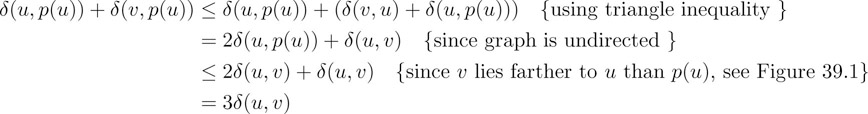
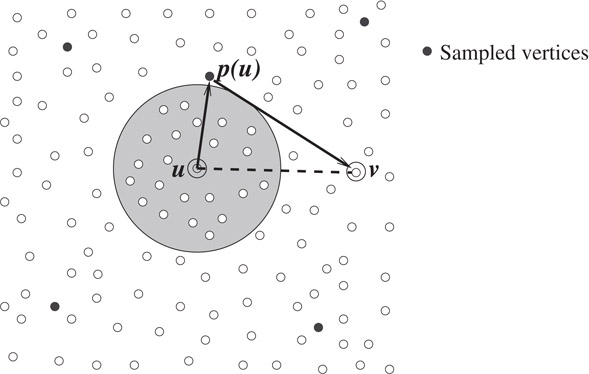
Figure 39.1v is farther to u than p(u), bounding δ(p(u),v) using triangle inequality.
Hence distance reported by the approximate distance oracle described above is no more than three times the actual distance between the two vertices. In other words, the oracle is a 3-approximate distance oracle. Now, we shall bound the expected size of the oracle. Using linearity of expectation, the expected size of the sample set R is nγ. Hence storing the distance from each vertex to all the vertices of sample set will take a total of O(n2γ) space. The following lemma gives a bound on the expected size of the sets Su, u ∈ V.
Lemma 39.1
Given a graph G = (V, E), let R ⊂ V be a set formed by picking each vertex independently with probability γ. For a vertex u ∈ V, the expected number of vertices in the set Su is bounded by 1/γ.
Proof. Let {v1, v2, …, vn−1} be the sequence of vertices of set V{u} arranged in non-decreasing order of their distance from u. The set Su consists of all those vertices of the set V{u} that lie closer to u than any vertex of set R. Note that the vertex vi belongs to Su if none of the vertices of set {v1, v2, …, vi−1} (i.e., the vertices preceding vi in the sequence above) is picked in the sample R. Since each vertex is picked independently with probability p, therefore the probability that vertex vi belongs to set Su is (1 − γ)i−1. Using linearity of expectation, the expected number of vertices lying closer to u than any sampled vertex is
Hence the expected number of vertices in the set Su is no more than 1/γ.
■
So the total expected size of the 3-approximate distance oracle is O(n2γ + n/γ). Choosing γ=1/√n
In the previous subsection, 3-approximate distance oracle was presented based on the idea I
Definition 39.1
For a vertex u, and subsets X, Y ⊂ V, the set Ball(u, X, Y ) is the set consisting of all those vertices of the set X that lie closer to u than any vertex from set Y. (see Figure 39.2)
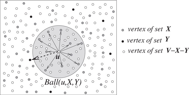
Figure 39.2The vertices pointed by solid-arrows constitute Ball(u, X, Y ).
It follows from the definition given above that Ball(u, X, ∅) is the set X itself, whereas Ball(u, X, X) = ∅. It can also be seen that the 3-approximate distance oracle described in the previous subsection stores Ball(u, V, R) and Ball(u, R, ∅) for each vertex u ∈ V.
If the set Y is formed by picking each vertex of set X independently with probability γ, it follows from Lemma 39.1 that the expected size of Ball(u, X, Y ) is bounded by 1/γ.
Lemma 39.2
Let G = (V, E) be a weighted graph, and X ⊂ V be a set of vertices. If Y ⊂ X is formed by selecting each vertex independently with probability γ, the expected number of vertices in Ball(u, X, Y ) for any vertex u ∈ V is at-most 1/γ.
39.2.3(2k - 1)-Approximate Distance Oracle
In this subsection we shall give the construction of a (2k − 1)-approximate distance oracle which is also based on the idea I
The (2k − 1)-approximate distance oracle is obtained as follows.
1.Let R1k⊃R2k⊃⋯Rkk
2.For each vertex u ∈ V, store the distance from u to all the vertices of Ball(u,Rkk,∅)
3.For each u ∈ V and each i < k, store the vertices of Ball(u,Rik,Ri+1k)
For sake of conciseness and without causing any ambiguity in notations, henceforth we shall use Balli(u) to denote Ball(u,Rik,Ri+1k)
The collection of the hash-tables Balli(u) : u ∈ V, i ≤ k constitute the data-structure that will facilitate answering of any approximate distance query in constant time. To provide a better insight into the data-structure, Figure 39.3 depicts the set of vertices constituting {Balli(u) | i ≤ k}.
Figure 39.3(i) Close description of Balli(u), i < k, (ii) hierarchy of balls around u.
39.2.3.1Reporting Distance with Stretch At-most (2k − 1)
Given any two vertices u, v ∈ V whose intermediate distance has to be determined approximately. We shall now present the procedure to find approximate distance between the two vertices using the k-level data-structure described above.
Let p1(u) = u and let pi(u), i > 1 be the vertex from the set Rik
The query answering process performs at-most k search steps. In the first step, we search Ball1(u) for the vertex p1(v). If p1(v) is not present in Ball1(u), we move to the next level and in the second step we search Ball2(v) for vertex p2(u). We proceed in this way querying balls of u and v alternatively : In ith step, we search Balli(x) for pi(y), where (x = u, y = v) if i is odd, and (x = v, y = u) otherwise. The search ends at ith step if pi(y) belongs to Balli(x), and then we report δ(x, pi(y)) + δ(y, pi(y) as an approximate distance between u and v.
Distance_Report (u, v)
Algorithm for reporting (2k − 1)-approximate distance between u, v ∈ V
l←1, x←u,y←v While (pl(y)≠Balll(x))(pl(y)≠Balll(x)) do swap(x, y), l←l + 1 return δ(y, pl(y)) + δ(x, pl(y))
Note that pk(y)∈Rkk
In order to ensure that the above algorithm reports (2k − 1)-approximate distance between u, v ∈ V, we first show that the following assertion holds:
Ai
The assertion Ai
For the base case (i = 0), p1(y) is same as y, and y is v. So δ(y, p1(y)) = 0. Hence A0
We consider the case of “even j,” the arguments for the case of “odd j” are similar. For even j, at the end of jth iteration, {x = u, y = v}, Thus Aj
Thus the assertion Aj+1
Theorem 39.1
The algorithm Distance_Report(u, v) reports (2k − 1)-approximate distance between u and v
Proof As an approximate distance between u and v, note that the algorithm Distance-Report(u, v) would output δ(y, pl(y)) + δ(x, pl(y)), which by triangle inequality is no more than 2δ(y, pl(y)) + δ(x, y). Since δ(x, y) = δ(u, v), and δ(y, pl(y)) ≤ (l − 1)δ(u, v) as follows from assertion Al
39.2.3.2Size of the (2k − 1)-approximate Distance Oracle
The expected size of the set Rkk
39.2.4Computing Approximate Distance Oracles
In this subsection, a sub-cubic running time algorithm is presented for computing (2k − 1)-approximate distance oracles. It follows from the description of the data-structure associated with approximate distance oracle that after forming the sampled sets of vertices Rik
Since Balli(u) is the set of all the vertices of set Rik
39.2.4.1Computing pi(u), ∀u ∈ V
Recall from definition itself that pi(u) is the vertex of the set Rik
Given X, Y ⊂ V in a graph G = (V, E), with X ∩ Y = ∅, compute the nearest vertex of set X for each vertex y ∈ Y.
The above problem can be solved by running a single source shortest path algorithm (Dijkstra’s algorithm) on a modified graph as follows. Modify the original graph G by adding a dummy vertex s to the set V, and joining it to each vertex of the set X by an edge of zero weight. Let G′ be the modified graph. Running Dijkstra’s algorithm from the vertex s as the source, it can be seen that the distance from s to a vertex y ∈ Y is indeed the distance from y to the nearest vertex of set X. Moreover, if e(s, x), x ∈ X is the edge leading to the shortest path from s to y, then x is the vertex from the set X that lies nearest to y. The running time of the Dijkstra’s algorithm is O(m log n), we can thus state the following lemma.
Lemma 39.3
Given X, Y ⊂ V in a graph G = (V, E), with X ∩ Y = ∅, it takes O(m log n) to compute the nearest vertex of set X for each vertex y ∈ Y.
Corollary 39.1
Given a weighted undirected graph G = (V, E), and a hierarchy of subsets {Rik|i≤k}
39.2.4.2Computing Balli(u) Efficiently
In order to compute Balli(u) for each vertex u ∈ V efficiently, we first compute clusters {C(v,Ri+1k)|v∈Rik}
Definition 39.2
For a graph G = (V, E), and a set X ⊂ V, the cluster C(v, X) consists of each vertex w ∈ V for whom v lies closer than any vertex of set X. That is, δ(w, v) < δ(w, x) for each x ∈ X.
It follows from the definition given above that u∈C(v,Ri+1k)
For each v∈Rikv∈Rik do For each u∈C(v,Ri+1k)u∈C(v,Ri+1k) do Balli(u)←Balli(u)∪{v}
Hence we can state the following Lemma.
Lemma 39.4
Given the family of clusters {C(v,Ri+1k)|v∈Rik}
The following property of the cluster C(v,Ri+1k)
Lemma 39.5
If u∈C(v,Ri+1k)
Proof. We give a proof by contradiction. Given that u∈C(v,Ri+1k)
Hence
Thus v does not lie closer to u than pi+1(w) which is a vertex of set Ri+1k
■
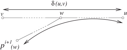
Figure 39.4if w does not lie in C(v,Ri+1k)
■
From Lemma 39.5, it follows that the graph induced by the vertices of the cluster C(v,Ri+1k)
A restricted Dijkstra’s algorithm: Note that the Dijkstra’s algorithm starts with singleton tree {v} and performs n − 1 steps to grow the complete shortest path tree. Each vertex x ∈ V{v} is assigned a label L(x), which is infinity in the beginning, but eventually becomes the distance from v to x. Let Vi denotes the set of i nearest vertices from v. The algorithm maintains the following invariant at the end of lth step:
I(l)
During the (j + 1)th step, we select the vertex, say w from set V − Vj with least value of L(·). Since all the edge weights are positive, it follows from the invariant I(j)
In the restricted Dijkstra’s algorithm, we will put the following restriction on relaxation of an edge e(w, y): we relax the edge e(w, y) only if L(w) + weight(w, y) is less than δ(y, pi(y)). This will ensure that a vertex y≠C(v,Ri+1k)
By Lemma 39.2, the expected size of Balli(x) is bounded by n1/k, hence using linearity of expectation, the total expected cost of computing {C(v,Ri+1k)|v∈Rik}
Using the above result and Lemma 39.4, we can thus conclude that for a given weighted graph G = (V, E) and an integer k, it takes a total of ˜O(kmn1/klogn)
Theorem 39.2
Given a weighted undirected graph G = (V, E) and an integer k, a data-structure of size O(kn1+1/k) can be built in O(kmn1/k) expected time so that given any pair of vertices, (2k − 1)-approximate distance between them can be reported in O(k) time.
39.3A Randomized Data-Structure for Decremental APASP
There are a number of applications that require efficient solutions of the APASP problem for a dynamic graph. In these applications, an initial graph is given, followed by an on-line sequence of queries interspersed with updates that can be insertion or deletion of edges. We have to carry out the updates and answer the queries on-line in an efficient manner. The goal of a dynamic graph algorithm is to update the solution efficiently after the dynamic changes, rather than having to re-compute it from scratch each time.
The approximate distance oracles described in the previous section can be used for answering approximate distance query in a static graph. However, there does not seem to be any efficient way to dynamize these oracles in order to answer distance queries in a graph under deletion of edges. In this section we shall describe a hierarchical data structure for efficiently maintaining APASP in an undirected unweighted graph under deletion of edges. In addition to maintaining approximate shortest paths for all-pairs of vertices, this scheme has been used for efficiently maintaining approximate shortest paths for pair of vertices separated by distance in an interval [a, b] for any 1 ≤ a < b ≤ n. However, to avoid giving too much detail in this chapter, we would outline an efficient algorithm for the following problem only.
APASP-d: Given an undirected unweighted graph G = (V, E) that is undergoing deletion of edges, and a distance parameter d ≤ n, maintain approximate shortest paths for all-pairs of vertices separated by distance at-most d.
For an undirected unweighted graph G = (V, E), a breadth-first-search (BFS) tree rooted at a vertex u ∈ V stores distance information with respect to the vertex u. So in order to maintain shortest paths for all-pairs of vertices separated by distance ≤ d, it suffices to maintain a BFS tree of depth d rooted at each vertex under deletion of edges. This is the approach taken by the previously existing algorithms.
The main idea underlying the hierarchical data-structure that would provide efficient update time for maintaining APASP can be summarized as follows: Instead of maintaining exact distance information separately from each vertex, keep small BFS trees around each vertex for maintaining distance information within locality of each vertex, and some what larger BFS trees around fewer vertices for maintaining global distance information.
We now provide the underlying intuition of the above idea and a brief outline of the new techniques used.
Let Bdu
In order to achieve o(nd) bound on the update time for the problem APASP-d, we closely look at the expression of total update time ∑u∈Vμ(Bdu)⋅d
•Is it possible to solve the problem APASP-d by keeping very few depth-d BFS trees?
•Is there some other alternative t for depth bounded BFS tree Bdu
While it appears difficult for any of the above ideas to succeed individually, they can be combined in the following way: Build and maintain BFS trees of depth 2d on vertices of a set S ⊂ V of size o(n), called the set of special vertices, and for each remaining vertex u ∈ VS, maintain a BFS tree (denoted by BSu
Along the above lines, we present a 2-level data-structure (and its generalization to k-levels) for the problem APASP-d.
It can be seen that unlike the tree Bdu
For our hierarchical scheme to lead to improved update time, it is crucial that we establish sub-linear upper bounds on μ(BSu)
For an undirected unweighted graph G = (V, E), S ⊂ V, and a distance parameter d ≤ n,
•δ(u, v): distance between u and v.
•N(v,S)
•Bdv
•BSv
•Bd,Sv
•μ(t): the number of edges in the sub-graph (of G) induced by the tree t.
•ν(t): the number of vertices in tree t.
•For a sequence {S0,S1,…Sk−1},Si⊂V
p0(u) = u.
pi+1(u) = the vertex from set Si+1 nearest to pi(u).
•¯α
39.3.3Hierarchical Distance Maintaining Data-Structure
Based on the idea of “keeping many small trees, and a few large trees,” we define a k-level hierarchical data-structure for efficiently maintaining approximate distance information as follows. (See Figure 39.5)
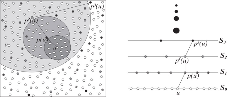
Figure 39.5Hierarchical scheme for maintaining approximate distance.
Let S={S0,S1,…,Sk−1:Si⊂V,|Si+1|<|Si|}
Let v be a vertex within distance d from u. If v is present in Bd,S1u
Lemma 39.6
Given a hierarchy Hkd
Proof. We give a proof by induction on j.
Base Case (j = 0): Since v is not present in BS1u
Induction Hypothesis:
δ(pi+1(u),pi(u))≤2iδ(u,v)
δ(pi+1(u),v)≤2i+1δ(u,v)
Induction Step (j = l): if v≠BSl+1pl(u)
Now using triangle inequality (see the Figure 39.6) we can bound δ(pl+1(u), v) as follows.
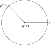
Figure 39.6Bounding the approximate distance between pi+1(u) and v.
■
Since the depth of a BFS tree at (k − 1)th level of hierarchy Hkd
Corollary 39.2
If δ(u, v) ≤ d, then there is some pi(u), i < k such that v is present in the BFS tree rooted at pi(u) in the hierarchy Hkd
Lemma 39.7
Given a hierarchy Hkd
Proof. Using simple triangle inequality, it follows that
■
It follows from Lemmas 39.6 and 39.7 that if l is the smallest integer such that v is present in the BFS tree rooted at pl(u) in the hierarchy Hkd
39.3.4Bounding the Size of Bd,Su
We shall now present a scheme based on random sampling to find a set S ⊂ V of vertices that will establish a sub-linear bound on the number of vertices (ν(BSu)
Build the set S of vertices by picking each vertex from V independently with probability ncn
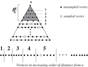
Figure 39.7Bounding the size of BFS tree BSu
To bound the number of edges induced by BSu
Note that in the sampling scheme to bound the number of vertices of tree BSu
R(c):Pick each vertexv∈Vindependently with probabilityncn+degree(v)⋅ncm.
It is easy to see that the expected size of the set formed by the sampling scheme R(c)
Theorem 39.3
Given an undirected unweighted graph G = (V, E), a constant c < 1, and a distance parameter d; a set S of size O(nc) vertices can be found that will ensure the following bound on the number of vertices and number of edges in the sub-graph of G induced by Bd,Su
with probability Ω(1−1n2)
39.3.4.1Maintaining the BFS Tree Bd,Su
Even and Shiloach [3] design an algorithm for maintaining a depth-d BFS tree in an undirected unweighted graph.
Lemma 39.8: (Even, Shiloach [3])
Given a graph under deletion of edges, a BFS tree Bdu,u∈V
For maintaining a Bd,Su
There are two computational tasks: one extending the level of the tree, and another that of maintaining the levels of the vertices in the tree Bd,Su
Lemma 39.9
Given an undirected unweighted graph G = (V, E) under edge deletions, a distance parameter d, and a set S ⊂ V; a BFS tree Bd,Su
amortized update time per edge deletion.
39.3.4.2Some Technical Details
As the edges are being deleted, we need an efficient mechanism to detect any increase in the depth of tree Bd,Su
For every vertex v ≠ S, we keep a count C[v] of the vertices of the S that are neighbors of v. It is easy to maintain C[u], ∀u ∈ V under edge-deletions. We use the count C[v] in order to detect any increase in the depth of a tree Bd,Su
Another technical issue is that when an edge e(x, y) is deleted, we must update only those trees which contain x and y. For this purpose, we maintain for each vertex, a set of roots of all the BFS trees containing it. We maintain this set using any dynamic search tree.
39.3.5Improved Decremental Algorithm for APASP up to Distance d
Let {(S0,F0),(S1,F1),…,(Sk−1,Fk−1)}
To report distance from u to v, we start form the level 0. We first inquire if v lies in Bd,S1u
Algorithm for reporting approximate distance using Hkd
Distance(u, v) { D←0;l←0 While (v≠B2ld,Sl+1pl(u)∧l<k−1v≠B2ld,Sl+1pl(u)∧l<k−1 ) do { If u∈B2ld,Sl+1pl(u), then D←δ(pl(u), u), D←D + δ(pl(u), pl+1(u)) l←l + 1; } If v≠B2ld,Sl+1pl(u), then “δ(u, v) is greater than d”, else return δ(pl(u), v) + D }
The approximation factor ensured by the above algorithm can be bounded as follows.
It follows from the Lemma 39.7 that the final value of D in the algorithm given above is bounded by (2l − 1)δ(u, v), and it follows from Lemma 39.6 that δ(pl(u), v) is bounded by 2lδ(u, v). Since l ≤ k − 1, therefore the distance reported by the algorithm is bounded by (2k − 1)δ(u, v) if v is at distance ≤ d.
Lemma 39.10
Given an undirected unweighted graph G = (V, E), and a distance parameter d. If α is the desired approximation factor, then there exists a hierarchical scheme Hkd with k=log2¯α, that can report α-approximate shortest distance between any two vertices separated by distance ≤ d, in time O(k).
Update time for maintaining the hierarchy Hdk: The update time per edge deletion for maintaining the hierarchy Hdk is the sum total of the update time for maintaining the set of BFS trees Fi,i≤k−1.
Each BFS tree from the set Fk−1 has depth 2k−1d, and edges O(m). Therefore, using Lemma 39.8, each tree from set Fk−1 requires O(2k−1d) amortized update time per edge deletion. So, the amortized update time Tk−1 per edge deletion for maintaining the set Fk−1 is
It follows from the Theorem 39.3 that a tree t from a set Fi,i<(k−1), has μ(t) = m ln n/nci+1, and depth =min{2id,nlnn/nci+1}. Therefore, using the Lemma 39.9, each tree t∈Fi,i<k−1 requires O(min{2id/nci+1,nlnn/n2ci+1}) amortized update time per edge deletion. So the amortized update time Ti per edge deletion for maintaining the set Fi is
Hence, the amortized update time T per edge deletion for maintaining the hierarchy Hdk is
To minimize the sum on right hand side in the above equation, we balance all the terms constituting the sum, and get
If α is the desired approximation factor, then it follows from Lemma 39.10 that the number of levels k, in the hierarchy are log2¯α. So the amortized update time required is ˜O(α⋅min{log2¯α√nd,(nd)¯α2(¯α−1)}).
Theorem 39.4
Let G = (V, E) be an undirected unweighted graph undergoing edge deletions, d be a distance parameter, and α > 2 be the desired approximation factor. There exists a data-structure ˙Dα(1,d) for maintaining α-approximate distances for all-pairs separated by distance ≤ d in ˜O(α⋅min{log2¯α√nd,(nd)¯α2(¯α−1)}) amortized update time per edge deletion, and O(log¯α) query time.
Based on the data-structure of [3], the previous best algorithm for maintaining all-pairs exact shortest paths of length ≤ d requires O(nd) amortized update time. We have been able to achieve o(nd) update time at the expense of introducing approximation as shown in Table 39.1 on the following page.
Table 39.1Maintaining α-approximate distances for all-pairs of vertices separated by distance ≤ d.
|
Data-structure |
α (the approximation factor) |
Amortized update time per edge deletion |
|
˙D3(1,d) |
3 |
˜O(min(√nd,(nd)2/3)) |
|
˙D7(1,d) |
7 |
˜O(min(3√nd,(nd)4/7)) |
|
˙D15(1,d) |
15 |
˜O(min(4√nd,(nd)8/15)) |
39.4Further Reading and Bibliography
Zwick [4] presents a very recent and comprehensive survey on the existing algorithms for all-pairs approximate/exact shortest paths. Based on the fastest known matrix multiplication algorithms given by Coppersmith and Winograd [5], the best bound for computing all-pairs shortest paths is O(n2.575) [6].
Approximate distance oracles are designed by Thorup and Zwick [7]. Based on a 1963 girth conjecture of Erdös [8], they also show that Ω(n1+1/k) space is needed in the worst case for any oracle that achieves stretch strictly smaller than (2k + 1). The space requirement of their approximate distance oracle is, therefore, essentially optimal. Also note that the preprocessing time of (2k − 1)-approximate distance oracle is O(mn1/k), which is sub-cubic. However, for further improvement in the computation time for approximate distance oracles, Thorup and Zwick pose the following question: Can (2k − 1)-approximate distance oracle be computed in ˜O(n2) time? Recently Baswana and Sen [9] answer their question in affirmative for unweighted graphs. However, the question for weighted graphs is still open.
For maintaining fully dynamic all-pairs shortest paths in graphs, the best known algorithm is due to Demetrescu and Italiano [10]. They show that it takes O(n2) amortized time to maintain all-pairs exact shortest paths after each update in the graph. Baswana et al. [11] present a hierarchical data-structure based on random sampling that provides efficient decremental algorithm for maintaining APASP in undirected unweighted graphs. In addition to achieving o(nd) update time for the problem APASP-d (as described in this chapter), they also employ the same hierarchical scheme for designing efficient data-structures for maintaining approximate distance information for all-pairs of vertices separated by distance in an interval [a, b], 1 ≤ a < b ≤ n.
The work of the first author is supported, in part, by a fellowship from Infosys Technologies Limited, Bangalore.
1.T.H. Cormen, C.E. Leiserson, and R.L. Rivest, Introduction to Algorithms, the MIT Press, 1990, chapter 12.
2.M.L. Fredman, J. Komlós, and E. Szemerédi, Storing a sparse table with O(1) worst case time, J. ACM, 31, 538, 1984.
3.S. Even and Y. Shiloach, An on-line edge-deletion problem, J. ACM, 28, 1, 1981.
4.U. Zwick, Exact and approximate distances in graphs - a survey, in Proc. of the 9th European Symposium on Algorithms (ESA), 2001, 33.
5.D. Coppersmith and S. Winograd, Matrix multiplication via arithmetic progressions, J. Symbolic Computation, 9, 251, 1990.
6.U. Zwick, All-pairs shortest paths in weighted directed graphs - exact and almost exact algorithms, in Proc. of the 39th IEEE Symposium on Foundations of Computer Science (FOCS), 1998, 310.
7.M. Thorup and U. Zwick, Approximate distance oracles, in Proc. of 33rd ACM Symposium on Theory of Computing (STOC), 2001, 183.
8.P. Erdös, Extremal problems in graph theory, in Theory of Graphs and its Applications (Proc. Sympos. Smolenice, 1963), Publ. House Czechoslovak Acad. Sci., Prague. 1964, 29.
9.S. Baswana and S. Sen, Approximate distance oracle for unweighted graphs in ˜O(n2) time, to appear in Proc. of the 15th Annual ACM-SIAM Symposium on Discrete Algorithms (SODA), 2004.
10.C. Demetrescu and G.F. Italiano, A new approach to dynamic all pairs shortest paths, in Proc. of 35th ACM Symposium on Theory of Computing (STOC), 2003, 159.
11.S. Baswana, R. Hariharan, and S. Sen, Maintaining all-pairs approximate shortest paths under deletion of edges, in Proc. of the 14th Annual ACM-SIAM Symposium on Discrete Algorithms (SODA), 2003, 394.
*This chapter has been reprinted from first edition of this Handbook, without any content updates.