
Peter Eades
University of Sydney
Seok-Hee Hong
University of Sydney
Barycenter Algorithm•Divide and Conquer Algorithm•Algorithm Using Canonical Ordering
Displaying Rotational Symmetry•Displaying Axial Symmetry•Displaying Dihedral Symmetry
Planar St-graphs•The Bar Visibility Algorithm•Bar Visibility Representations and Layered Drawings•Bar Visibility Representations for Orthogonal Drawings
Graph Drawing is the art of making pictures of relationships. For example, consider the social network defined in Table 47.1. This table expresses the “has-written-a-joint-paper-with” relation for a small academic community.
It is easier to understand this social network if we draw it. A drawing is in Figure 47.1a; a better drawing is in Figure 47.1b. The challenge for Graph Drawing is to automatically create good drawings of graphs such as in Figure 47.1b, starting with tables such as in Table 47.1.
Table 47.1Table Representing the has-a-joint-paper-with Relation
|
Name |
has-a-joint-paper-with |
|
Jane |
Harry, Paula, and Sally |
|
Sally |
Jane, Paula and Dennis |
|
Dennis |
Sally and Monty |
|
Harry |
Jane and Paula |
|
Monty |
Dennis and Kerry |
|
Ying |
Paula |
|
Paula |
Jane, Harry, Ying, Tan, Cedric, Chris, Kerry and Sally |
|
Kerry |
Paula and Monty |
|
Tan |
Paul and Cedric |
|
Cedric |
Tan, Paula, and Chris |
|
Chris |
Paula and Cedric |
The criteria of a good drawing of a graph have been the subject of a great deal of attention (see, e.g., [1–3]). The four criteria below are among the most commonly used criteria.
•Edge crossings should be avoided. Human tests clearly indicate that edge crossings inhibit the readability of the graph [3]. Figure 47.1a has 6 edge crossings, and Figure 47.1b has none; this is the main reason that Figure 47.1b is more readable than Figure 47.1a. The algorithms presented in this chapter deal with planar drawings, that is, drawings with no edge crossings.
•The resolution of a graph drawing should be as large as possible. There are several ways to define the intuitive concept of resolution; the simplest is the vertex resolution, that is, the ratio of the minimum distance between a pair of vertices to the maximum distance between a pair of vertices. High resolution helps readability because it allows a larger font size to be used in the textual labels on vertices. In practice it can be easier to measure the area of the drawing, given that the minimum distance between a pair of vertices is one. If the vertices in Figure 47.1 are on an integer grid, then the drawing is 4 units by 2 units, for both (a) and (b). Thus the vertex resolution is , and the area is 8. One can refine the concept of resolution to define edge resolution and angular resolution.
•The symmetry of the drawing should be maximized. Symmetry conveys the structure of a graph, and Graph Theory textbooks commonly use drawings that are as symmetric as possible. Intuitively, Figure 47.1b displays more symmetry than Figure 47.1a. A refined concept of symmetry display is presented in Section 47.4.
•Edge bends should be minimized. There is some empirical evidence to suggest that bends inhibit readability. In Figure 47.1a, three edges contain bends and eleven are straight lines; in total, there are seven edge bends. Figure 47.1b is much better: all edges are straight lines.
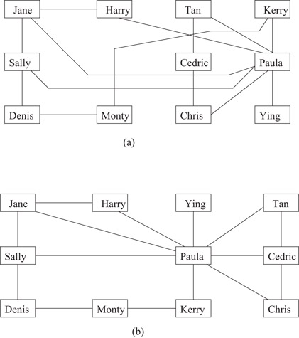
Figure 47.1Two drawings of a social network.
Each of these criteria can be measured. Thus Graph Drawing problems are commonly stated as optimization problems: given a graph G, we need to find a drawing of G for which one or more of these measures are optimal. These optimization problems are usually NP-complete.
In most cases it is not possible to optimize one of the criteria above without compromise on another. For example, the graph in Figure 47.2a has 8 symmetries but one edge crossing. It is possible to draw this graph without edge crossings, but in this case we can only get 6 symmetries, as in Figure 47.2b.
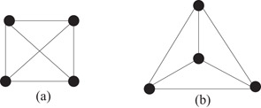
Figure 47.2Two drawings of a graph.
The optimization problem may be constrained. For example, consider a graph representing prerequisite dependencies between the units in a course, as in Figure 47.3; in this case, the y coordinate of a unit depends on the semester in which the unit ought to be taken.
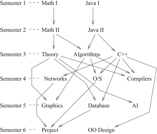
Figure 47.3Prerequisite diagram.
Graph Drawing has a long history in Mathematics, perhaps beginning with the theorem of Wagner that every planar graph can be drawn with straight line edges [4]. The importance of graph drawing algorithms was noted early in the history of Computer Science (note the paper of Knuth on drawing flowcharts, in 1960 [5], and the software developed by Read in the 1970s [6]). In the 1980s, the availability of graphics workstations spawned a broad interest in visualization in general and in graph visualization in particular. The field became mature in the mid 1990s with a conference series (e.g., see the annual proceedings of Symposium on Graph Drawing), some books [7–10], and widely available software (see Reference 11).
In this chapter we briefly describe just a few of the many graph available drawing algorithms. Section 47.3 presents some algorithms to draw planar graphs with straight line edges and convex faces. Section 47.4 describes two algorithms that can be used to construct planar symmetric drawings. Section 47.5 presents a method for constructing “visibility” representations of planar graphs, and shows how this method can be used to construct drawings with few bends and reasonable resolution.
Basic concepts of mathematical Graph Theory are described in Reference 12. In this section we define mathematical notions that are used in many Graph Drawing algorithms.
A drawing D of a graph G = (V, E) assigns a location D(u) ∈ R2 for every vertex u ∈ V and a curve D(e) in R2 for every edge e ∈ E such that if e = (u, v) then the curve D(e) has endpoints D(u) and D(v). If D(u) has integer coordinates for each vertex u, then D is a grid drawing. If the curve D(e) is a straight line segment for each edge e, then D is a straight line drawing.
For convenience we often identify the vertex u with its location D(u), and the edge e with its corresponding curve D(e); for example, when we say “the edge e crosses the edge f,”strictly speaking we should say “the curve D(e) crosses the curve D(f).” A graph drawing is planar if adjacent edges intersect only at their common endpoint, and no two nonadjacent edges intersect. A graph is planar if it has a planar drawing. Planarity is a central concern of Graph Theory, Graph Algorithms, and especially Graph Drawing; see Reference 12.
A planar drawing of a graph divides the plane into regions called faces. One face is unbounded; this is the outside face. Two faces are adjacent if they share a common edge. The graph G together its faces and the adjacency relationship between the faces is a plane graph. The graph whose vertices are the faces of a plane graph G and whose edges are the adjacency relationships between faces is the planar dual, or just dual, of G. A graph and its planar dual are in Figure 47.4.
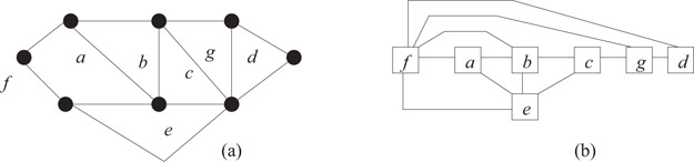
Figure 47.4(a) A graph G and its faces. (b) The dual of G.
The neighborhood N(u) of a vertex u is the list of vertices that are adjacent to u. If G is a plane graph, then N(u) is given in the clockwise circular ordering about u.
A straight-line drawing of a planar graph is convex if all every face is drawn as convex polygon. This section reviews three different algorithms for constructing such a drawing for planar graphs.
Tutte showed that a convex drawing exist for triconnected planar graphs and gave an algorithm for constructing such representations [13,14].
The algorithm divides the vertex set V into two subsets; a set of fixed vertices and a set of free vertices. The fixed vertices are placed at the vertices of a strictly convex polygon. The positions of free vertices are decided by solving a system of O(n) linear equations, where n is the number of vertices of the graph [14]. In fact, solving the equations is equivalent to placing each free vertex at the barycenter of its neighbors. That is, each position p(v) = (x(v), y(v)) of a vertex v is:
(47.1) |
|---|
An example of a drawing computed by the barycenter algorithm is illustrated in Figure 47.5. Here the black vertices represent fixed vertices.
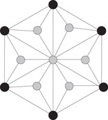
Figure 47.5Example output from the algorithm of Tutte.
The main theorem can be described as follows.
Suppose that f is a face in a planar embedding of a triconnected planar graph G, and P is a strictly convex planar drawing of f. Then the barycenter algorithm with the vertices of f fixed and positioned according to P gives a convex planar drawing of G.
The matrix resulting from the equations can be solved in O(n1.5) time at best, using a sophisticated sparse matrix elimination method [15]. However, in practice a Newton-Raphson iteration of the equation above converges rapidly.
47.3.2Divide and Conquer Algorithm
Chiba, Yamanouchi and Nishizeki [16] present a linear time algorithm for constructing convex drawings of planar graphs, using divide and conquer. The algorithm constructs a convex drawing of a planar graph, if it is possible, with a given outside face. The drawing algorithm is based on a classical result by Thomassen [17].
The input to their algorithm is a biconnected plane graph with given outside face and a convex polygon. The output of their algorithm is a convex drawing of the biconnected plane graph with outside face drawn as the input convex polygon, if this is possible. The conditions under which such a drawing is possible come from the following theorem [17].
Theorem 47.2: (Thomassen [17])
Let G be a biconnected plane graph with outside facial cycle S, and let S* be a drawing of S as a convex polygon. Let P1, P2, …, Pk be the paths in S, each corresponding to a side of S*. (Thus S* is a k-gon. It should be noted that not every vertex of the cycle S is necessarily an apex of the polygon S*.) Then S* can be extended to a convex drawing of G if and only if the following three conditions hold.
1.For each vertex v of G − V (S) having degree at least three in G, there are three paths disjoint except at v, each joining v and a vertex of S;
2.The graph G − V (S) has no connected component C such that all the vertices on S adjacent to vertices in C lie on a single path Pi; and no two vertices in each Pi are joined by an edge not in S; and
3.Any cycle of G which has no edge in common with S has at least three vertices of degree at least 3 in G.
The basic idea of the algorithm of Chiba et al. [16] is to reduce the convex drawing of G to those of several subgraphs of G as follows:
Algorithm ConvexDraw(G, S, S*)
1.Delete from G an arbitrary apex v of S* together with edges incident to v.
2.Divide the resulting graph G′ = G − v into the biconnected components B1, B2, …, Bp.
3.Determine a convex polygon for the outside facial cycle Si of each Bi so that Bi with satisfies the conditions in Theorem 47.2.
4.Recursively apply the algorithm to each Bi with to determine the positions of vertices not in Si.
The main idea of the algorithm is illustrated in Figure 47.6; for more details see Reference 16.
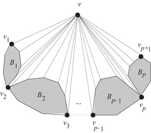
Figure 47.6The algorithm of Chiba et al.
It is easy to show that the algorithm runs in linear time, and its correctness can be established using Theorem 47.2.
Theorem 47.3: (Chiba, Yamanouchi and Nishizeki [16])
Algorithm ConvexDraw constructs a convex planar drawing of a biconnected plane graph with given outside face in linear time, if such a drawing is possible.
47.3.3Algorithm Using Canonical Ordering
Both the Tutte algorithm and the algorithm of Chiba et al. give poor resolution. Kant [18] gives a linear time algorithm for constructing a planar convex grid drawing of a triconnected planar graph on a (2n − 4) × (n − 2) grid, where n is the number of vertices. This guarantees that the vertex resolution of the drawing is Ω(1/n).
Kant’s algorithm is based on a method of de Fraysseix, Pach and Pollack [19] for drawing planar triangulated graphs on a grid of size (2n − 4) × (n − 2).
The algorithm of de Fraysseix et al. [19] computes a special ordering of vertices called the canonical ordering based on fixed embedding. Then the vertices are added, one by one, in order to construct a straight-line drawing combined with shifting method. Note that the outside face of the drawing is always triangle, as shown in Figure 47.7.
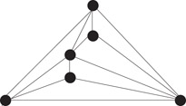
Figure 47.7Planar straight-line grid drawing given by de Fraysseix, Pach and Pollack method.
Kant [18] uses a generalization of the canonical ordering called leftmost canonical ordering. The main difference from the algorithm of de Fraysseix et al. [19] is that it gives a convex drawing of triconnected planar graph. The following Theorem summarizes his main result.
Theorem 47.4: (Kant [18])
There is a linear time algorithm to construct a planar straight-line convex drawing of a triconnected planar graph with n vertices on a (2n − 4) × (n − 2) grid.
Details of Kant’s algorithm are in Reference [18]. Chrobak and Kant improved the algorithm so that the size of the grid is (n − 2) × (n − 2) [20].
A graph drawing can have two kinds of symmetry: axial (or reflectional) symmetry and rotational symmetry. For example, see Figure 47.8. The drawing in Figure 47.8a displays four rotational symmetries and Figure 47.8b displays one axial symmetry. Figure 47.8c displays eight symmetries, four rotational symmetries as well as four axial symmetries.
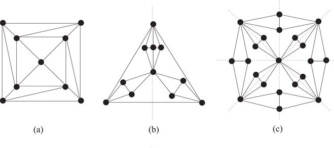
Figure 47.8Three symmetric drawings of graphs.
Manning [21] showed that, in general, the problem of determining whether a given graph can be drawn symmetrically is NP-complete. De Fraysseix [22] presents heuristics for symmetric drawings of general graphs. Exact algorithms for finding symmetries in general graphs were presented by Buchheim and Junger [23], and Abelson, Hong and Taylor [24].
There are linear time algorithms available for restricted classes of graphs. Manning and Atallah present a liner time algorithm for detecting symmetries in trees [25] and outerplanar graphs [26]. Hong, Eades and Lee present a linear time algorithm for drawing series-parallel digraphs symmetrically [27]. A linear time algorithm for drawing planar graphs with maximum number of symmetries are given by Hong, McKay and Eades [28] for triconnected planar graphs, by Hong and Eades for biconnected planar graphs [29], and oneconnected planar graphs [30], and disconnected planar graphs [31]. Recently, a linear time algorithm for symmetric convex drawings of internally-triconnected planar graphs are given by Hong and Nagamochi [32]. For a recent survey on symmetric graph drawing, see Reference 33.
In this section, we briefly describe a linear time algorithm to draw triconnected planar graphs with maximum symmetry. Note that the algorithm of Tutte described in Section 47.3.1 can be used to construct symmetric drawings of triconnected planar graphs, but it does not work in linear time. Here we give the linear time algorithm of Hong, McKay and Eades [28]. It has two steps:
1.Symmetry finding: this step finds symmetries, or so-called geometric automorphisms [24,34], in graphs.
2.Symmetric drawing: this step constructs a drawing that displays these automorphisms.
More specifically, the symmetry finding step finds a plane embedding that displays the maximum number of symmetries. It is based on a classical theorem from group theory called the orbit-stabilizer theorem [35]. It also uses a linear time algorithm of an algorithm of Fontet [36] to compute orbits and generators for groups of geometric automorphisms. For details, see Reference 28. Here we present only the second step, that is, the drawing algorithm. This constructs a straight-line planar drawing of a given triconnected plane graph such that given symmetries are displayed.
The drawing algorithm has three routines, each corresponding to a type of group of symmetries in two dimensions:
1.The cyclic case: displaying k rotational symmetries;
2.One axial case: displaying one axial symmetry;
3.The dihedral case: displaying 2k symmetries (k rotational symmetries and k axial symmetries).
The dihedral case is important for displaying maximum number of symmetries, however it is the most difficult to achieve. Here, we concentrate on the first two cases; the cyclic case and the one axial case. In Section 47.4.1, we describe an algorithm for constructing a drawing displaying rotational symmetry and in Section 47.4.2 we describe an algorithm for constructing a drawing displaying axial symmetry. We briefly comments on the dihedral case in Section 47.4.3.
The input of the drawing algorithm is a triconnected plane graph; note that the outside face is given. Further, the algorithm needs to compute a triangulation as a preprocessing step. More specifically, given a plane embedding of triconnected planar graphs with a given outside face, we triangulate each internal face by inserting a new vertex in the face and joining it to each vertex of the face. This process is called star-triangulation and clearly it takes only linear time.
A major characteristic of symmetric drawings is the repetition of congruent drawings of isomorphic subgraphs. The algorithms use this property, that is, they compute a drawing for a subgraph and then use copies of it to draw the whole graph. More specifically, each symmetric drawing algorithm consists of three steps. First, it finds a subgraph. Then it draws the subgraph using the algorithm of Chiba et al. [16] as a subroutine. The last step is to replicate the drawing; that is, merge copies of the subgraphs to construct a drawing of the whole graph.
The application of Theorem 47.2 is to subgraphs of a triconnected plane graph defined by a cycle and its interior. In that case Thomassen’s conditions can be simplified. Suppose that P is a path in a graph G; a chord for P in G is an edge (u, v) of G not in P, but whose endpoints are in P.
Corollary 47.1
Let G be a triconnected plane graph and let S be a cycle of G. Let W be the graph consisting of S and its interior. Let S* be a drawing of S as a convex k-gon (where S might have more than k vertices). Let P1, P2, …, Pk be the paths in S corresponding to the sides of S*. Then S* is extendable to a straight-line planar drawing of W if and only if no path Pi has a chord in W.
Proof. We can assume that the interior faces of W are triangles, since otherwise we can star triangulate them.
We need to show that Thomassen’s three conditions are met. Condition 1 is a standard implication of the triconnectivity of G, and Condition 3 follows just from the observation that the internal vertices have degree at least 3.
To prove the first part of Condition 2, suppose on the contrary that C is a connected component of W − S which is adjacent to Pi but not to any other of P1, …, Pk. Let u and v be the first and last vertices on Pi which are adjacent to C. If u = v, or u and v are adjacent on Pi, then {u, v} is a cut (separation pair) in G, which is impossible as G is triconnected. Otherwise, there is an interior face containing u and v and so u and v are adjacent contrary to our hypothesis (since the internal faces are triangles).
The second part of Condition 2 is just the condition that we are imposing.■
47.4.1Displaying Rotational Symmetry
Firstly, we consider the cyclic case, that is, displaying k rotational symmetries. Note that after the star-triangulation, we may assume that there is either an edge or a vertex fixed by the symmetry. The fixed edge case can only occur if k = 2 and this case can be transformed into the fixed vertex case by inserting a dummy vertex into the fixed edge with two dummy edges. Thus we assume that there is a fixed vertex c.
The symmetric drawing algorithm for the cyclic case consists of three steps.
Algorithm Cyclic
1.Find_Wedge_Cyclic.
2.Draw_Wedge_Cyclic.
3.Merge_Wedges_Cyclic.
The first step is to find a subgraph W, called a wedge, as follows.
Algorithm Find_Wedge_Cyclic
1.Find the fixed vertex c.
2.Find a shortest path P1, from c to a vertex v1 on the outside face. This can be done in linear time by breadth first search.
3.Find the path P2 which is a mapping of P1 under the rotation.
4.Find the induced subgraph of G enclosed by the cycle formed from P1, P2 and a path P0 along the outside face from v1 to v2 (including the cycle). This is the wedge W.
A wedge W is illustrated in Figure 47.9a. It is clear that Algorithm Find_Wedge_Cyclic runs in linear time.
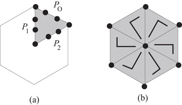
Figure 47.9Example of (a) a wedge and (b) merging.
The second step, Draw_Wedge_Cyclic, constructs a drawing D of the wedge W using Algorithm ConvexDraw, such that P1 and P2 are drawn as straight-lines. This is possible by the next lemma.
Lemma 47.1
Suppose that W is the wedge computed by Algorithm Find_Wedge_Cyclic, S is the outside face of W, and S* is the drawing of the outside face S of W using three straight-lines as in Figure 47.9a. Then S* is extendable to a planar straight-line drawing of W.
Proof. One of the three sides of S* corresponds to part of the outside face of G, which cannot have a chord as G is triconnected. The other two sides cannot have chords either, as they are shortest paths in G. Thus W and S* satisfy the conditions of Corollary 47.1.
■
The last step, Merge_Wedges_Cyclic, constructs a drawing of the whole graph G by replicating the drawing D of W, k times. Note that this merge step relies on the fact that P1 and P2 are drawn as straight-lines. This is illustrated in Figure 47.9b.
Clearly, each of these three steps takes linear time. Thus the main result of this section can be stated as follows.
Theorem 47.5
Algorithm Cyclic constructs a straight-line drawing of a triconnected plane graph which shows k rotational symmetry in linear time.
47.4.2Displaying Axial Symmetry
A critical element of the algorithm for displaying one axial symmetry is the subgraph that is fixed by the axial symmetry. Consider a drawing of a star-triangulated planar graph with one axial symmetry. There are fixed vertices, edges and/or fixed faces on the axis. The subgraph formed by these vertices, edges and faces, is called a fixed string of diamonds.
The first step of the algorithm is to identify the fixed string of diamonds. Then the second step is to use Algorithm Symmetric_ConvexDraw, a modified version of Algorithm ConvexDraw. Thus Algorithm One_Axial can be described as follows.
Algorithm One_Axial
1.Find a fixed string of diamonds. Suppose that ω1, ω2, …, ωk are the fixed edges and vertices in the fixed string of diamonds, in order from the outside face (ω1 is on the outside face). For each ℓ, ωℓ may be a vertex or an edge. This is illustrated in Figure 47.10.
2.Choose an axially symmetric convex polygon S* for the outside face of G.
3.Symmetric_ConvexDraw(1, S*, G).
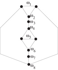
Figure 47.10A string of diamonds.
The main subroutine in Algorithm One_Axial is Algorithm Symmetric_ConvexDraw. This algorithm, described below, modifies Algorithm ConvexDraw so that the following three conditions are satisfied.
1.Choose v in Step 1 of Algorithm ConvexDraw to be ω1. In Algorithm ConvexDraw, v must be a vertex; here we extend Algorithm ConvexDraw to deal with an edge or a vertex. The two cases are illustrated in Figure 47.11.
2.Let D(Bi) be the drawing of Bi and α be the axial symmetry. Then, D(Bi) should be a reflection of D(Bj), where Bj = α(Bi), i = 1, 2, …, m and m = ⌊p/2⌋.
3.If p is odd, then D(Bm+1) should display one axial symmetry.
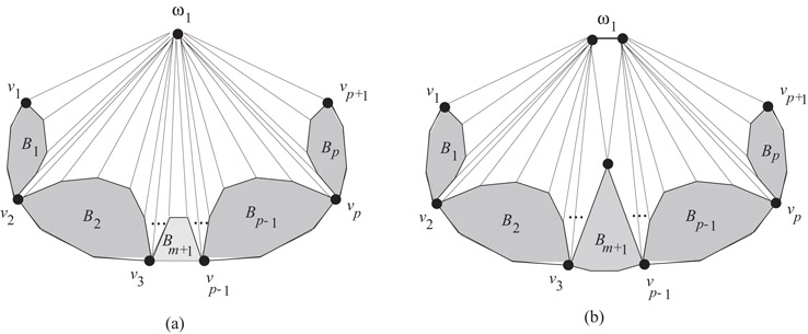
Figure 47.11Symmetric version of ConvexDraw.
It is easy to see that satisfying these three conditions ensures the display a single axial symmetry.
Let Bj = α(Bi). The second condition can be achieved as follows. First define to be the reflection of , i = 1, 2, …, m. Then apply Algorithm ConvexDraw for Bi, i = 1, 2, …, m and construct D(Bj) using a reflection of D(Bi). If p is odd then we recursively apply Algorithm Symmetric_ConvexDraw to Bm + 1. Thus Algorithm Symmetric_ConvexDraw can be described as follows.
Algorithm Symmetric_ConvexDraw(ℓ, S*, G)
1.Delete ωℓ from G together with edges incident to ωℓ. Divide the resulting graph G′ = G − ωℓ into the blocks B1, B2, …, Bp, ordered anticlockwise around the outside face. Let m = ⌊p/2⌋.
2.For each i = 1 to m, determine a convex polygon of the outside facial cycle Si of each Bi so that Bi with satisfy the conditions in Theorem 47.2 and chose to be a reflection of .
3.For each i = 1 to m,
a.Construct a drawing D(Bi) of Bi using Algorithm ConvexDraw.
b.Construct D(Bp−i+1) as a reflection of D(Bi).
4.If p is odd, then construct a drawing D(Bm+1) using Symmetric_ConvexDraw().
5.Merge the D(Bi) to form a drawing of G.
Using the same argument as for the linearity of Algorithm ConvexDraw [16], one can show that Algorithm One_Axial takes linear time.
Theorem 47.6
Algorithm One_Axial constructs a straight-line drawing of a triconnected plane graph which shows one axial symmetry in linear time.
47.4.3Displaying Dihedral Symmetry
In this section, we briefly review an algorithm for constructing a drawing displaying k axial symmetries and k rotational symmetries.
As with the cyclic case, we assume that there is a vertex fixed by all the symmetries. The algorithm adopts the same general strategy as for the cyclic case: divide the graph into “wedges,” draw each wedge, then merge the wedges together to make a symmetric drawing. However, the dihedral case is more difficult than the pure rotational case, because an axial symmetry in the dihedral case can have fixed edges and/or fixed faces. This requires a much more careful applications of the Algorithm ConvexDraw and Algorithm Symmetric_ConvexDraw; for details see Reference 28.
Nevertheless, using three steps above, a straight-line drawing of a triconnected plane graph which shows dihedral symmetry can be constructed in linear time.
In conclusion, the symmetry finding algorithm together with the three drawing algorithms ensures the following theorem which summarizes their main result.
Theorem 47.7: (Hong, McKay and Eades [28])
There is a linear time algorithm that constructs maximally symmetric planar drawings of triconnected planar graphs, with straight-line edges.
In general, a visibility representation of a graph has a geometric shape for each vertex, and a “line of sight” for each edge. Different visibility representations involve different kinds of geometric shapes and different restrictions on the “line of sight.” A three dimensional visibility representation of the complete graph on five vertices is in Figure 47.12. Here the geometric objects are rectangular prisms, and each “line of sight” is parallel to a coordinate axis.
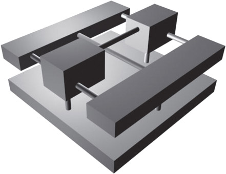
Figure 47.12A visibility representation in three dimensions (courtesy of Nathalie Henry).
Visibility representations have been extensively investigated in both two and three dimensions.
For two dimensional graph drawing, the simplest and most common visibility representation uses horizontal line segments (called “bars”) for vertices and vertical line segments for “lines of sight.” More precisely, a bar visibility representation of a graph G = (V, E) consists of a horizontal line segment ωu for each vertex u ∈ V, and a vertical line segment λe for each edge e ∈ E, such that the following properties hold:
•If u and u′ are distinct vertices of G, then ωu has empty intersection with ωu′.
•If e and e′ are distinct edges of G, then λe has empty intersection with λe′.
•If e is not incident with u then λe has empty intersection with ωu.
•If e is incident with u then the intersection of λe and ωu consists of an endpoint of λe on ωu.
Figure 47.13 shows a bar visibility representation of the 3-cube.

Figure 47.13A bar visibility representation of the 3-cube.
It is clear that if G admits a bar visibility representation, then G is planar. Tamassia and Tollis [37] and Rosenstiehl and Tarjan [38] proved the converse: every planar graph has a bar visibility representation. Further, they showed that the resulting drawing has quadratic area, that is, the resolution is good. The algorithms from [37] and [38] construct such a representation in linear time.
In the Section 47.5.1 below we describe some concepts used to present the algorithm. Section 47.5.2 describes the basic algorithm for constructing bar visibility representations, and Sections 47.5.3 and 47.5.4 show how to apply these representations to obtain layered drawings and orthogonal drawings respectively.
The algorithm in Section 47.5.2 and some of the preceding results are stated in terms of biconnected planar graphs. Note that this restriction can be avoided by augmenting graphs of lower connectivity with dummy edges.
Bar visibility representation algorithms use the theory of planar st-graphs. This is a powerful theory which is useful in a variety of graph drawing applications. In this section we describe enough of this theory to allow presentation of a bar visibility algorithm; for proofs of the results here, and more details about planar st-graphs, see Reference 7.
A directed plane graph is a planar st-graph if it has one source s and one sink t, and both s and t are on the outside face. We say that a vertex u on a face f of a planar st-graph is a source for f (respectively sink for f) if the edges incident with u on f are out-edges (respectively in-edges).
Lemma 47.2
Every face f of a planar st-graph has one source sf for f and one sink tf for f.
We need to extend the concept of the “planar dual,” defined in Section 47.2, to directed graphs. For a directed plane graph G, the directed dual G* has a vertex vf for each internal face f of G, as well as two vertices ℓext and rext for the external face of G.
To define the edges of G*, we must first define the left and right side face of each edge of G. Suppose that f is an internal face of G, and the cycle of edges traversing f in a clockwise direction is (e1, e2, …, ek). The clockwise traversal may pass through some edges in the same direction as the edge, and some edges in the opposite direction. If we pass through ei in the same direction as ei then we define right(ei) = vf; if we pass through ej in the opposite direction to ej then we define left(ej) = vf.
Now consider a clockwise traversal (e′1, e′2, …, e′k) of the external face of G. If we pass through e′i in the same direction as e′i then we define left(ei) = ℓext; if we pass through ej in the opposite direction to ej then we define right(ej) = rext.
One can easily show that the definitions of left and right are well founded, that is, that for each edge e there is precisely one face f of G such that left(e) = vf and precisely one one face f′ of G such that right(e) = vf′.
For each edge e of G, G* has an edge from left(e) to right(e).
An example is in Figure 47.14. Here ℓext = 1 = left(e), and rext = 5 = right(j) = right(g), left(f) = left(i) = 2, right(f) =right(h) = 4, and left(h) = right(i) = 3.
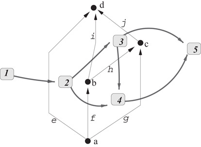
Figure 47.14A directed planar graph and its directed dual.
The following Lemma (see Reference 7 for a proof) is important for the bar visibility algorithm.
Lemma 47.3
Suppose that f and f′ are faces in a planar st-graph G. Then precisely one of the following statements is true.
a.There is a directed path in G from the sink of f to the source of f′.
b.There is a directed path in G from the sink of f′ to the source of f.
c.There is a directed path in G* from vf to vf′.
d.There is a directed path in G* from vf′ to vf.
The next Lemma is, in a sense, dual to Lemma 47.2.
Lemma 47.4
Suppose that u is a vertex in a planar st-graph. The outgoing edges from u are consecutive in the circular ordering of N(u), and the incoming edges are consecutive in the circular ordering of N(u).
Lemma 47.4 leads to a definition of the left and right of a vertex. Suppose that (e1, e2, …, ek) is the circular list of edges around a non-source non-sink vertex u, in clockwise order. From Lemma 47.4, for some i, edge ei comes into u and edge ei+1 goes out from u. we say that ei is the leftmost in-edge of u and ei+1 is the leftmost out-edge of u. If f is the face shared by ei and ei+1 then we define left(u) = f. Similarly, there is a j such that edge ej goes out from u and edge ej+1 comes into u; we say that ej is the rightmost out-edge of u and ej+1 is the rightmost in-edge of u. If f′ is shared by ej and ej+1 then we define right(ej) = f′. If u is either the source or the sink, then left(u) = ℓext and right(u) = rext.
In Figure 47.14, for example, left(a) = left(d) = 1, left(b) = 2, left(c) = 3, right(b) = 4, and right(a) = right(c) = right(d) = 5.
Finally, we need the following Lemma, which is a kind of dual to Lemma 47.3.
Lemma 47.5
Suppose that u and u′ are vertices in G. Then precisely one of the following statements is true.
a.There is a directed path in G from u to u′.
b.There is a directed path in G from u′ to u.
c.There is a directed path in G* from right(u) to left(u′).
d.There is a directed path in G* from right(u′) to left(u).
47.5.2The Bar Visibility Algorithm
The bar visibility algorithm takes a biconnected plane graph as input, and converts it to a planar st-graph. Then it computes the directed dual, and a “topological number” (defined below) for each vertex in both the original graph and the dual. Using these numbers, it assigns a y coordinate for each vertex and an x coordinate for each edge. The bar representing the vertex extends far enough to touch each incident edge, and the vertical line representing the edge extends far enough to touch each the bars representing its endpoints.
If G = (V, E) is an acyclic directed graph with n vertices, a topological numbering Z of G assigns an integer Z(u) ∈ {0, 1, …, n − 1} to every vertex u ∈ V such that Z(u) < Z(v) for all directed edges (u, v) ∈ E. Note that we do not require that the function Z be one-one, that is, it is possible that two vertices are assigned the same number.
The algorithm is described below.
      Algorithm Bar_Visibility
      Input: a biconnected plane graph G = (V, E)
      Output: a bar visibility representation of G
1.Choose two vertices s and t of G on the same face.
2.Direct the edges of G so that s is the only source, t is the only sink, and the resulting digraph is acyclic.
3.Compute a topological numbering Y for G.
4.Compute the directed planar dual G* = (V*, E*) of G.
5.Compute a topological numbering X for G*.
6.For each vertex u, let ωu be the line segment .
7.For each edge e = (u, v), let λe be the line segment .
Step 2 can be implemented by a simple variation on the depth-first-search method, based on a biconnectivity algorithm.
There are many kinds of topological numberings for acyclic digraphs: for example, one can define Z(u) to be the number of edges in the longest path from the source s to u. Any of these methods can be used in steps 3 and 5.
Theorem 47.8: (Tamassia and Tollis [37]; Rosenstiehl and Tarjan [38])
A visibility representation of a biconnected planar graph with area O(n) × O(n) can be computed in linear time.
Proof. We need to show that the drawing defined by ω and λ in Algorithm Bar_Visibility satisfies the four properties P1, P2, P3 and P4 above.
First consider P1, and suppose that u and u′ are two vertices of G. If Y (u) ≠ Y (u′) then ωu has empty intersection with ωu′ and so P1 holds. Now suppose that Y (u) = Y (u′). Since Y is a topological numbering of G, it follows that there is no directed path in between u and u′ (in either direction). Thus, from Lemma 47.5, in G* either there is a directed path from right(u) to left(u′) or a directed path from right(u′) to left(u). The first case implies that X(right(u)) < X(left(u′), so that the whole of ωu is to the left of ωu′; the second case implies that the whole of ωu′ is to the left of ωu. This implies P1.
Now consider P2, and suppose that e = (u, v) and e′ = (u′, v′) are edges of G, and denote left(e) by f and left(e′) by f′. If X(f) ≠ X(f′) then λe cannot intersect λe′ and P2 holds. Now suppose that X(f) = X(f′); thus in G* there is no directed path between f and f′. It follows from Lemma 47.3 that in G either there is a directed path from the sink tf of f to the source sf′ of f′, or a directed path from the sink tf′ of f′ to the source sf of f. In the first case we have Y (tf) < Y (sf′). Also, since e is on f and e′ is on f′, we have Y (v) ≤ Y (tf) and Y (sf′) ≤ Y (u′); thus Y (v) < Y (u′) and λe cannot intersect λe′. The second case is similar and so P2 holds.
A similar argument shows that P3 holds.
Property P4 follows form the simple observation that for any edge e = (u, v), X(left(u)) ≤ X(left(e)) ≤ X(right(u)).
The drawing has dimensions , which is O(n) × O(n).
It is easy to see that each step can be implemented in linear time.■
47.5.3Bar Visibility Representations and Layered Drawings
A graph in which the nodes are constrained to specified y coordinates, as in Figure 47.3, is called a layered graph. More precisely, a layered graph consists of a directed graph G = (V, E) as well as a topological numbering L of G. We say that L(u) is the layer of u. A drawing of G that satisfies the layering constraint, that is, the y coordinate of u is L(u) for each u ∈ V, is called a layered drawing. Drawing algorithms for layered graphs have been extensively explored [7].
A layered graph is planar (sometimes called h-planar) if it can be drawn with no edge crossings, subject to the layering constraint. Note that underlying the prerequisite Figure 47.3 is a planar graph; however, as a layered graph, it is not planar. The theory of planarity for layered graphs has received some attention; see References 39–42.
If a planar layered graph has one source and one sink, then it is a planar st-graph. Clearly the source s has and the sink t has . Since the layers define a topological numbering of the graph, application of Algorithm Bar_Visibility yields a visibility representation that satisfies the layering constraints. Further, this can be used to construct a graph drawing by using simple local transformations, illustrated in Figure 47.15.
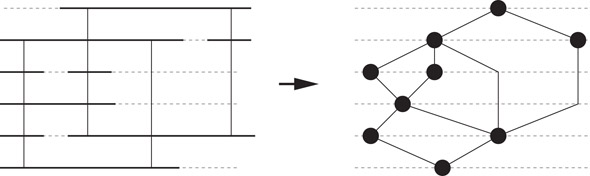
Figure 47.15Transformation from a visibility representation of a layered graph to a layered drawing.
The following theorem is immediate.
Theorem 47.9
If G is a planar layered graph then we can construct a planar layered drawing of G in linear time, with the following properties:
•There are at most two bends in each edge.
•The area is O(n) × O(n).
Although Algorithm Bar_Visibility produces the visibility representation with good resolution, it may not produce minimum area drawings. Lin and Eades [42] give a linear time variation on Algorithm Bar Visibility that, for a fixed embedding, maximizes resolution. The algorithm works by using a topological numbering for the dual computed from a dependency relation between the edges.
47.5.4Bar Visibility Representations for Orthogonal Drawings
An orthogonal drawing of a graph G has each vertex represented as a point and each edge represented by a polyline whose line segments are parallel to a coordinate axis. An orthogonal drawing of the 3-cube is in Figure 47.16.

Figure 47.16An orthogonal drawing of the 3-cube.
It is clear that a graph that has a planar orthogonal drawing, has maximum degree of G at most 4. Conversely, one can obtain a planar orthogonal drawing of a planar graph with maximum degree at most 4 from a visibility representation by using a simple set of local transformations, described in Figure 47.17.
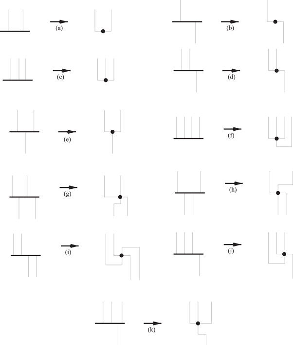
Figure 47.17Local transformations to transform a visibility representation to an orthogonal drawing.
Figure 47.16 can be obtained from Figure 47.13 by applying transformation (c) in Figure 47.17 to the source and sink, and applying transformation (d) to each other vertex.
Note that the transformations involve the introduction of a few bends in each edge. The worst case is for where a transformation introduces two bends near a vertex; this may occur at each end of an edge, and thus may introduce 4 bends into an edge.
Theorem 47.10
If G is a planar graph then we can construct a planar orthogonal drawing of G in linear time, with the following properties:
•There are at most four bends in each edge.
•The area is O(n) × O(n).
In fact, a variation of Algorithm Visibility together with a careful application of some transformations along the lines of those in Figure 47.17 can ensure that the resulting drawing has a total of at most 2n + 4 bends, where n is the number of vertices; see Reference 7.
In this chapter we have described just a small sample of graph drawing algorithms. Notable omissions include:
•Force directed methods: A graph can be used to define a system of forces. For example, we can define a Hooke’s law spring force between two adjacent vertices, and magnetic repulsion between nonadjacent vertices. A minimum energy configuration of the graph can lead to a good drawing. For methods using the force-directed paradigm, see References 7–10, 43.
•Clustered graph drawing: in practice, to handle large graphs, one needs to form clusters of the vertices to form “super-vertices.” Drawing graphs in which some vertices represent graphs is a challenging problem. For algorithms drawing clustered graphs, see References 8,40.
•Three dimensional graph drawing: the widespread availability of cheap three dimensional graphics systems has lead to the investigation of graph drawing in three dimensions. For algorithms drawing graphs in three dimensions, see References 8,10, 44.
•Crossing minimization methods: in this chapter we have concentrated on planar graphs. In practice, we need to deal with non-planar graphs, by choosing a drawing with a small number of crossings. For algorithms drawing non-planar graphs with crossing minimization methods, see References 7–10, 45,46.
•Generalization of convex drawing: Note that graphs admit convex drawings if and only if they are internally-triconnected [16,17]. In practice, we need to relax and generalize convex drawings to “good” non-convex drawings for biconnected graphs. For algorithms drawing planar graphs with non-convex boundary constraints (such as star-shaped boundary), called inner convex drawings, see Reference 47. For algorithms drawing biconnected planar graphs with star-shaped faces, called star-shaped drawings, see Reference 48; algorithms for star-shape drawings with minimum number of concave corners, see References 49,50. For algorithms drawing biconnected planar graphs with non-convex polytopes in three dimensions, called upward star-shaped polytopes, see Reference 51.
•Beyond planar graphs: Recently, the problem of drawing non-planar graphs with specific types of crossing constraints or forbidden crossing constraints, called beyond planar graphs and beyond planarity, have been studied [52–57]. This include k-planar graphs, that is, graphs that can be drawn in the plane with at most k crossings per edge. For algorithms testing beyond planarity and drawing beyond planar graphs, see Reference 56 for drawing 1-planar graphs, see Reference 53 for drawing almost planar graphs, see Reference 54 for testing maximal-1-planar graphs, see Reference 55 for testing outer-1-planar graphs, see Reference 52 for testing maximal-outer-fanplanar graphs, and see Reference 57 for testing full-outer-2-planar graphs.
1.C. Batini, E. Nardelli and R. Tamassia, A Layout Algorithm for Data-Flow Diagrams, IEEE Trans. Softw. Eng., SE-12(4), 538–546, 1986.
2.J. Martin and C. McClure. Diagramming Techniques for Analyst and Programmers. Prentice Hall Inc., Michigan, 1985.
3.H. Purchase, Which Aesthetic Has the Greatest Effect on Human Understanding, Proceedings of Graph Drawing 1997, Lecture Notes in Computer Science 1353, Springer-Verlag, pp. 248–261, 1998.
4.K. Wagner, Bemerkungen zum Vierfarbenproblem, Jahres-bericht der Deutschen Mathematiker-Vereinigung, 46, pp. 26–32, 1936.
5.D. E. Knuth, Computer Drawn Flowcharts, Commun, ACM, 6, pp. 555–563, 1963.
6.R. Read, Some Applications of Computers in Graph Theory, In L.W. Beineke, R. Wilson, Selected Topics in Graph Theory, chapter 15, pp. 415–444. Academic Press, 1978.
7.G. Di Battista, P. Eades, R. Tamassia and I. G. Tollis. Graph Drawing: Algorithms for the Visualization of Graphs. Prentice-Hall, 1998.
8.M. Kaufmann and D. Wagner Eds., Drawing Graphs - Methods and Models, Lecture Notes in Computer Science 2025, 2001.
9.K. Sugiyama. Graph Drawing and Applications for Software and Knowledge Engineers. Series on Software Engineering and Knowledge Engineering - Vol. 11, World Scientific, 2002.
10.R. Tamassia. Handbook on Graph Drawing and Visualization. Chapman and Hall, CRC, 2013.
11.M. Junger and P. Mutzel Eds., Graph Drawing Software, Series: Mathematics and Visualization, Springer-Verlag, 2003.
12.J. A. Bondy and U. S. R. Murty, Graph Theory with Applications, MacMillan Press, London, 1977.
13.W. T. Tutte, Convex Representations of Graphs, Proc. London Math. Soc., 10, pp. 304–320, 1960.
14.W. T. Tutte, How to Draw a Graph, Proc. London Math. Soc., 13, pp. 743–768, 1963.
15.R. J. Lipton, D. J. Rose and R. E. Tarjan, Generalized Nested Dissection, SIAM J. Numer. Anal., 16(2), pp. 346–358, 1979.
16.N. Chiba, T. Yamanouchi and T. Nishizeki, Linear Algorithms for Convex Drawings of Planar Graphs, In J.A. Bondy and U.S.R. Murty, Progress in Graph Theory, Academic Press, pp. 153–173, 1984.
17.C. Thomassen, Planarity and Duality of Finite and Infinite Graphs, J. of Combinatorial Theory, Series B, 29, pp. 244–271, 1980.
18.G. Kant, Drawing Planar Graphs Using the Canonical Ordering, Algorithmica, 16, pp. 4–32, 1996.
19.H. de Fraysseix, J. Pach and R. Pollack, How to Draw a Planar Graph on a Grid, Combinatorica, 10, pp. 41–51, 1990.
20.M. Chrobak and G. Kant, Convex Grid Drawings of 3-connected Planar Graphs, Int. Journal of Computational Geometry and Applications, 7(3), 211–224, 1997.
21.J. Manning, Geometric Symmetry in Graphs, Ph.D. Thesis, Purdue Univ., 1990.
22.H. de Fraysseix, An Heuristic for Graph Symmetry Detection, Proceedings of Graph Drawing 1999, Lecture Notes in Computer Science 1731, Springer-Verlag, pp. 276–285, Springer-Verlag, 1999.
23.C. Buchheim and M. Jünger, Detecting Symmetries by Branch and Cut, Math. Program., 98(1–3), 369–384, 2003.
24.D. Abelson, S. Hong and D. E. Taylor, Geometric Automorphism Groups of Graphs, Discrete Applied Mathematics, 155(17), 2211–2226, 2007.
25.J. Manning and M. J. Atallah, Fast Detection and Display of Symmetry in Trees, Congressus Numerantium, 64, pp. 159–169, 1988.
26.J. Manning and M. J. Atallah, Fast Detection and Display of Symmetry in Outerplanar Graphs, Discrete Applied Mathematics, 39, pp. 13–35, 1992.
27.S. Hong, P. Eades and S. Lee, Drawing Series Parallel Digraphs Symmetrically, Computational Geometry: Theory and Applicatons, 17(3–4), pp. 165–188, 2000.
28.S. Hong, B. D. McKay and P. Eades, A Linear Time Algorithm for Constructing Maximally Symmetric Straight Line Drawings of Triconnected Planar Graphs, Discrete and Computational Geometry, 36(2), pp. 283–311, 2006.
29.S. Hong and P. Eades, Drawing Planar Graphs Symmetrically II: Biconnected Planar Graphs, Algorithmica, 42(2), pp. 159–197, 2005.
30.S. Hong and P. Eades, Drawing Planar Graphs Symmetrically III: Oneconnected Planar Graphs, Algorithmica, 44(1), pp. 67–100, 2006.
31.S. Hong and P. Eades, Symmetric Layout of Disconnected Graphs, Proceedings of ISAAC 2003, LNCS, Kyoto, Japan, pp. 405–414, 2003.
32.S. Hong and H. Nagamochi, A Linear-Time Algorithm for Symmetric Convex Drawings of Internally Triconnected Plane Graphs, Algorithmica, 58(2), pp. 433–460, 2010.
33.P. Eades and S. Hong, Symmetric Graph Drawing, In R. Tamassia, Handbook on Graph Drawing and Visualization, pp. 87–113, 2013.
34.P. Eades and X. Lin, Spring Algorithms and Symmetry, Theoretical Computer Science, 240(2), pp. 379–405, 2000.
35.M. A. Armstrong, Groups and Symmetry, Springer-Verlag, 1988.
36.M. Fontet, Linear Algorithms for Testing Isomorphism of Planar Graphs, Proceedings of Third Colloquium on Automata, Languages, and Programming, pp. 411–423, 1976.
37.R. Tamassia and I. G. Tollis, A Unified Approach to Visibility Representations of Planar Graphs, Discrete and Computational Geometry, 1(4), pp. 321–341, 1986.
38.P. Rosenstiehl and R. E. Tarjan, Rectilinear Planar Layouts and Bipolar Orientations of Planar Graphs, Discrete and Compututational Geometry, 1(4), pp. 342–351, 1986.
39.P. Eades, X. Lin and R. Tamassia, An Algorithm for Drawing a Hierarchical Graph, International Journal of Computational Geometry and Applications, 6(2), pp. 145–155, 1996.
40.P. Eades, Q. Feng, X. Lin and H. Nagamochi, Straight-Line Drawing Algorithms for Hierarchical Graphs and Clustered Graphs, Algorithmica, 44(1), pp. 1–32, 2006.
41.M. Junger, S. Leipert and P. Mutzel, Level Planarity Testing in Linear Time, Proceedings of Graph Drawing 1998, Lecture Notes in Computer Science 1547, Stirin Castle, Czech Republic, Springer-Verlag, pp. 167–182, 1999.
42.X. Lin and P. Eades, Towards Area Requirements for Drawing Hierarchically Planar Graphs, Theoretical Computer Science, 292(3), pp. 679–695, 2003.
43.S. G. Kobourov, Force-Directed Drawing Algorithms, In R. Tamassia, Handbook on Graph Drawing and Visualization, pp. 383–408, 2013.
44.V. Dujmovic, Three-Dimensional Drawings, In R. Tamassia, Handbook on Graph Drawing, Visualization, pp. 455–488, 2013.
45.C. Buchheim, M. Chimani, C. Gutwenger, M. Jnger and P. Mutzel, Crossings and Planarization, In R. Tamassia, Handbook on Graph Drawing and Visualization, pp. 43–85, 2013.
46.P. Healy and N. S. Nikolov, Hierarchical Drawing Algorithms, In R. Tamassia, Handbook on Graph Drawing and Visualization, pp. 409–453, 2013.
47.S. Hong and H. Nagamochi, Convex Drawings of Graphs with Non-convex Boundary Constraints, Discrete Applied Mathematics, 156(12), pp. 2368–2380, 2008.
48.S. Hong and H. Nagamochi, An Algorithm for Constructing Star-shaped Drawings of Plane Graphs, Compututational Geometry: Theory and Application, 43(2), pp. 191–206, 2010.
49.S. Hong and H. Nagamochi, A Linear-Time Algorithm for Star-Shaped Drawings of Planar Graphs with the Minimum Number of Concave Corners, Algorithmica, 62(3-4), pp. 1122–1158, 2012.
50.S. Hong and H. Nagamochi, Minimum Cost Star-shaped Drawings of Plane Graphs with a Fixed Embedding and Concave Corner Constraints, Theoretical Computer Science, 445, pp. 36–51, 2012.
51.S. Hong and H. Nagamochi, Extending Steinitz’s Theorem to Upward Star-Shaped Polyhedra and Spherical Polyhedra, Algorithmica, 61(4), pp. 1022–1076, 2011.
52.M. A. Bekos, S. Cornelsen, L. Grilli, S. Hong and M. Kaufmann, On the Recognition of Fan-Planar and Maximal Outer-Fan-Planar Graphs, Proceedings of Graph Drawing 2014, Wuezburg, Germany, pp. 198–209, 2014.
53.P. Eades, S. Hong, G. Liotta, N. Katoh and S. Poon, Straight-Line Drawability of a Planar Graph Plus an Edge, Proceedings of WADS 2015, Victoria, Canada, pp. 301–313, 2015.
54.P. Eades, S. Hong, N. Katoh, G. Liotta, P. Schweitzer and Y. Suzuki, A Linear Time Algorithm for Testing Maximal 1-planarity of Graphs with a Rotation System, Theoretical Computer Science, 513, pp. 65–76, 2013.
55.P. Eades, S. Hong, N. Katoh, G. Liotta, P. Schweitzer and Y. Suzuki, A Linear-Time Algorithm for Testing Outer-1-Planarity, Algorithmica, 72(4), pp. 1033–1054, 2015.
56.S. Hong, P. Eades, G. Liotta and S. Poon, Fry’s Theorem for 1-Planar Graphs, Proceedings of COCOON 2012, LNCS, Sydney, Australia, pp. 335–346, 2012.
57.S. Hong and H. Nagamochi, Testing Full-outer-2-planarity in Linear Time, In E. Mayr, Proceedings of WG 2015, LNCS, Garching, Germany, pp. 406–421, 2015.
*This chapter has been reprinted from first edition of this Handbook, without any content updates.