49. IP Router Tables

An Internet router classifies incoming packets into flows^‡ utilizing information contained in packet headers and a table of (classification) rules. This table is called the rule table (equivalently, router table). The packet-header information that is used to perform the classification is some subset of the source and destination addresses, the source and destination ports, the protocol, protocol flags, type of service, and so on. The specific header information used for packet classification is governed by the rules in the rule table. Each rule-table rule is a pair of the form (F, A), where F is a filter and A is an action. The action component of a rule specifies what is to be done when a packet that satisfies the rule filter is received. Sample actions are drop the packet, forward the packet along a certain output link, and reserve a specified amount of bandwidth. A rule filter F is a tuple that is comprised of one or more fields. In the simplest case of destination-based packet forwarding, F has a single field, which is a destination (address) prefix and A is the next hop for packets whose destination address has the specified prefix. For example, the rule (01 * , a) states that the next hop for packets whose destination address (in binary) begins with 01 is a. IP (Internet Protocol) multicasting uses rules in which F is comprised of the two fields source prefix and destination prefix; QoS routers may use five-field rule filters (source-address prefix, destination-address prefix, source-port range, destination-port range, and protocol); and firewall filters may have one or more fields.

In the d-dimensional packet classification problem, each rule has a d-field filter. In this chapter, we are concerned solely with 1-dimensional packet classification. It should be noted, that data structures for multidimensional packet classification are usually built on top of data structures for 1-dimensional packet classification. Therefore, the study of data structures for 1-dimensional packet classification is fundamental to the design and development of data structures for d-dimensional, d > 1, packet classification.

For the 1-dimensional packet classification problem, we assume that the single field in the filter is the destination field and that the action is the next hop for the packet. With these assumptions, 1-dimensional packet classification is equivalent to the destination-based packet forwarding problem. Henceforth, we shall use the terms rule table and router table to mean tables in which the filters have a single field, which is the destination address. This single field of a filter may be specified in one of two ways:

1.As a range. For example, the range [35, 2096] matches all destination addresses d such that 35 ≤ d ≤ 2096.

2.As an address/mask pair. Let x_i denote the ith bit of x. The address/mask pair a/m matches all destination addresses d for which d_i = a_i for all i for which m_i = 1. That is, a 1 in the mask specifies a bit position in which d and a must agree, while a 0 in the mask specifies a don’t care bit position. For example, the address/mask pair 101100/011101 matches the destination addresses 101100, 101110, 001100, and 001110.

When all the 1-bits of a mask are to the left of all 0-bits, the address/mask pair specifies an address prefix. For example, 101100/110000 matches all destination addresses that have the prefix 10 (i.e., all destination addresses that begin with 10). In this case, the address/mask pair is simply represented as the prefix 10*, where the * denotes a sequence of don’t care bits. If W is the length, in bits, of a destination address, then the * in 10* represents all sequences of W − 2 bits. In IPv4 the address and mask are both 32 bits, while in IPv6 both of these are 128 bits.

Notice that every prefix may be represented as a range. For example, when W = 6, the prefix 10* is equivalent to the range [32,47]. A range that may be specified as a prefix for some W is called a prefix range. The specification 101100/011101 may be abbreviated to ?011?0, where ? denotes a don’t-care bit. This specification is not equivalent to any single range. Also, the range specification [3,6] isn’t equivalent to any single address/mask specification.

Figure 49.1 shows a set of five prefixes together with the start and finish of the range for each. This figure assumes that W = 5. The prefix P1 = *, which matches all legal destination addresses, is called the default prefix.

Figure 49.1Prefixes and their ranges.

Suppose that our router table is comprised of five rules R1–R5 and that the filters for these five rules are P1–P5, respectively. Let N1–N5, respectively, be the next hops for these five rules. The destination address 18 is matched by rules R1, R3, and R5 (equivalently, by prefixes P1, P3, and P5). So, N1, N3, and N5 are candidates for the next hop for incoming packets that are destined for address 18. Which of the matching rules (and associated action) should be selected? When more than one rule matches an incoming packet, a tie occurs. To select one of the many rules that may match an incoming packet, we use a tie breaker.

Let RS be the set of rules in a rule table and let FS be the set of filters associated with these rules. rules(d, RS) (or simply rules(d) when RS is implicit) is the subset of rules of RS that match/cover the destination address d. filters(d, FS) and filters(d) are defined similarly. A tie occurs whenever |rules(d)| > 1 (equivalently, |filters(d)| > 1).

Three popular tie breakers are:

1.First matching rule in table. The rule table is assumed to be a linear list [1] of rules with the rules indexed 1 through n for an n-rule table. The action corresponding to the first rule in the table that matches the incoming packet is used. In other words, for packets with destination address d, the rule of rules(d) that has least index is selected.

For our example router table corresponding to the five prefixes of Figure 49.1, rule R1 is selected for every incoming packet, because P1 matches every destination address. When using the first-matching-rule criteria, we must index the rules carefully. In our example, P1 should correspond to the last rule so that every other rule has a chance to be selected for at least one destination address.

2.Highest-priority rule. Each rule in the rule table is assigned a priority. From among the rules that match an incoming packet, the rule that has highest priority wins is selected. To avoid the possibility of a further tie, rules are assigned different priorities (it is actually suﬃcient to ensure that for every destination address d, rules(d) does not have two or more highest-priority rules).

Notice that the first-matching-rule criteria is a special case of the highest-priority criteria (simply assign each rule a priority equal to the negative of its index in the linear list).

3.Most-specific-rule matching. The filter F1 is more specific than the filter F2 iff F2 matches all packets matched by F1 plus at least one additional packet. So, for example, the range [2, 4] is more specific than [1, 6], and [5, 9] is more specific than [5, 12]. Since [2, 4] and [8, 14] are disjoint (i.e., they have no address in common), neither is more specific than the other. Also, since [4, 14] and [6, 20] intersect,^* neither is more specific than the other. The prefix 110* is more specific than the prefix 11*.

In most-specific-rule matching, ties are broken by selecting the matching rule that has the most specific filter. When the filters are destination prefixes, the most-specific-rule that matches a given destination d is the longest^* prefix in filters(d). Hence, for prefix filters, the most-specific-rule tie breaker is equivalent to the longest-matching-prefix criteria used in router tables. For our example rule set, when the destination address is 18, the longest matching-prefix is P4. When the filters are ranges, the most-specific-rule tie breaker requires us to select the most specific range in filters(d). Notice also that most-specific-range matching is a special case of the the highest-priority rule. For example, when the filters are prefixes, set the prefix priority equal to the prefix length. For the case of ranges, the range priority equals the negative of the range size.

In a static rule table, the rule set does not vary in time. For these tables, we are concerned primarily with the following metrics:

1.Time required to process an incoming packet. This is the time required to search the rule table for the rule to use.

2.Preprocessing time. This is the time to create the rule-table data structure.

3.Storage requirement. That is, how much memory is required by the rule-table data structure?

In practice, rule tables are seldom truly static. At best, rules may be added to or deleted from the rule table infrequently. Typically, in a “static” rule table, inserts/deletes are batched and the rule-table data structure reconstructed as needed.

In a dynamic rule table, rules are added/deleted with some frequency. For such tables, inserts/deletes are not batched. Rather, they are performed in real time. For such tables, we are concerned additionally with the time required to insert/delete a rule. For a dynamic rule table, the initial rule-table data structure is constructed by starting with an empty data structures and then inserting the initial set of rules into the data structure one by one. So, typically, in the case of dynamic tables, the preprocessing metric, mentioned above, is very closely related to the insert time.

In this paper, we focus on data structures for static and dynamic router tables (1-dimensional packet classification) in which the filters are either prefixes or ranges.

49.2Longest Matching-Prefix

49.2.1Linear List

In this data structure, the rules of the rule table are stored as a linear list[1] L. Let LMP(d) be the longest matching-prefix for address d. LMP(d) is determined by examining the prefixes in L from left to right; for each prefix, we determine whether or not that prefix matches d; and from the set of matching prefixes, the one with longest length is selected. To insert a rule q, we first search the list L from left to right to ensure that L doesn’t already have a rule with the same filter as does q. Having verified this, the new rule q is added to the end of the list. Deletion is similar. The time for each of the operations determine LMP(d), insert a rule, delete a rule is O(n), where n is the number of rules in L. The memory required is also O(n).

Note that this data structure may be used regardless of the form of the filter (i.e., ranges, Boolean expressions, etc.) and regardless of the tie breaker in use. The time and memory complexities are unchanged.

Although the linear list is not a suitable data structure for a purely software implementation of a router table with a large number of prefixes, it is leads to a very practical solution using TCAMs (ternary content-addressable memories) [2,3]. Each memory cell of a TCAM may be set to one of three states 0, 1, and don’t care. The prefixes of a router table are stored in a TCAM in descending order of prefix length. Assume that each word of the TCAM has 32 cells. The prefix 10* is stored in a TCAM word as 10???…?, where ? denotes a don’t care and there are 30 ?s in the given sequence. To do a longest-prefix match, the destination address is matched, in parallel, against every TCAM entry and the first (i.e., longest) matching entry reported by the TCAM arbitration logic. So, using a TCAM and a sorted-by-length linear list, the longest matching-prefix can be determined in O(1) time. A prefix may be inserted or deleted in O(W) time, where W is the length of the longest prefix [2].^† For example, an insert of a prefix of length 3 (say) can be done by relocating a the first prefix of length 1 to the end of the list; filling the vacated slot with the first prefix of length 2; and finally filling this newly vacated spot with the prefix of length 3 that is to be inserted.

Despite the simplicity and eﬃciency of using TCAMs, TCAMs present problems in real applications [4]. For example, TCAMs consume a lot of power and board area.

49.2.2End-Point Array

Lampson, Srinivasan, and Varghese [5] have proposed a data structure in which the end points of the ranges defined by the prefixes are stored in ascending order in an array. LMP(d) is found by performing a binary search on this ordered array of end points.

Prefixes and their ranges may be drawn as nested rectangles as in Figure 49.2a, which gives the pictorial representation of the five prefixes of Figure 49.1.

Figure 49.2(a) Pictorial representation of prefixes and ranges (b) Array for binary search.

In the data structure of Lampson et al. [5], the distinct range end-points are stored in ascending order as in Figure 49.2b. The distinct end-points (range start and finish points) for the prefixes of Figure 49.1 are [0, 10, 11, 16, 18, 19, 23, 31]. Let r_i, 1 ≤ i ≤ q ≤ 2n be the distinct range end-points for a set of n prefixes. Let r_q+1 = ∞. With each distinct range end-point, r_i, 1 ≤ i ≤ q, the array stores LMP(d) for d such that (a) r_i < d < r_i+1 (this is the column labeled “> ” in Figure 49.2b and (b) r_i = d (column labeled “=”). Now, LMP(d), r1 ≤ d ≤ r_q can be determined in O(log n) time by performing a binary search to find the unique i such that r_i ≤ d < r_i+1. If r_i = d, LMP(d) is given by the “=” entry; otherwise, it is given by the “> ” entry. For example, since d = 20 satisfies 19 ≤ d < 23 and since d ≠ 19, the “> ” entry of the end point 19 is used to determine that LMP(20) is P1.

As noted by Lampson et al. [5], the range end-point table can be built in O(n) time (this assumes that the end points are available in ascending order). Unfortunately, as stated in Reference 5, updating the range end-point table following the insertion or deletion of a prefix also takes O(n) time because O(n) “> ” and/or “=” entries may change. Although Lampson et al. [5] provide ways to reduce the complexity of the search for the LMP by a constant factor, these methods do not result in schemes that permit prefix insertion and deletion in O(log n) time.

It should be noted that the end-point array may be used even when ties are broken by selecting the first matching rule or the highest-priority matching rule. Further, the method applies to the case when the filters are arbitrary ranges rather than simply prefixes. The complexity of the preprocessing step (i.e., creation of the array of ordered end-points) and the search for the rule to use is unchanged. Further, the memory requirements are the same, O(n) for an n-rule table, regardless of the tie breaker and whether the filters are prefixes or general ranges.

49.2.3Sets of Equal-Length Prefixes

Waldvogel et al. [6] have proposed a data structure to determine LMP(d) by performing a binary search on prefix length. In this data structure, the prefixes in the router table T are partitioned into the sets S0, S1, … such that S_i contains all prefixes of T whose length is i. For simplicity, we assume that T contains the default prefix. *So, S0 = { * }. Next, each S_i is augmented with markers that represent prefixes in S_j such that j > i and i is on the binary search path to S_j. For example, suppose that the length of the longest prefix of T is 32 and that the length of LMP(d) is 22. To find LMP(d) by a binary search on length, we will first search S16 for an entry that matches the first 16 bits of d. This search^* will need to be successful for us to proceed to a larger length. The next search will be in S24. This search will need to fail. Then, we will search S20 followed by S22. So, the path followed by a binary search on length to get to S22 is S16, S24, S20, and S22. For this to be followed, the searches in S16, S20, and S22 must succeed while that in S24 must fail. Since the length of LMP(d) is 22, T has no matching prefix whose length is more than 22. So, the search in S24 is guaranteed to fail. Similarly, the search in S22 is guaranteed to succeed. However, the searches in S16 and S20 will succeed iff T has matching prefixes of length 16 and 20. To ensure success, every length 22 prefix P places a marker in S16 and S20, the marker in S16 is the first 16 bits of P and that in S20 is the first 20 bits in P. Note that a marker M is placed in S_i only if S_i doesn’t contain a prefix equal to M. Notice also that for each i, the binary search path to S_i has O(log l_max) = O(log W), where l_max is the length of the longest prefix in T, S_js on it. So, each prefix creates O(log W) markers. With each marker M in S_i, we record the longest prefix of T that matches M (the length of this longest matching-prefix is necessarily smaller than i).

To determine LMP(d), we begin by setting leftEnd = 0 and rightEnd = l_max. The repetitive step of the binary search requires us to search for an entry in S_m, where m = ⌊(leftEnd + rightEnd)/2⌋, that equals the first m bits of d. If S_m does not have such an entry, set rightEnd = m − 1. Otherwise, if the matching entry is the prefix P, P becomes the longest matching-prefix found so far. If the matching entry is the marker M, the prefix recorded with M is the longest matching-prefix found so far. In either case, set leftEnd = m + 1. The binary search terminates when leftEnd > rightEnd.

One may easily establish the correctness of the described binary search. Since, each prefix creates O(log W) markers, the memory requirement of the scheme is O(n log W). When each set S_i is represented as a hash table, the data structure is called SELPH (sets of equal length prefixes using hash tables). The expected time to find LMP(d) is O(log W) when the router table is represented as an SELPH. When inserting a prefix, O(log W) markers must also be inserted. With each marker, we must record a longest-matching prefix. The expected time to find these longest matching-prefixes is O(log2W). In addition, we may need to update the longest-matching prefix information stored with the O(n log W) markers at lengths greater than the length of the newly inserted prefix. This takes O(n log2W) time. So, the expected insert time is O(n log2W). When deleting a prefix P, we must search all hash tables for markers M that have P recorded with them and then update the recorded prefix for each of these markers. For hash tables with a bounded loading density, the expected time for a delete (including marker-prefix updates) is O(n log2W). Waldvogel et al. [6] have shown that by inserting the prefixes in ascending order of length, an n-prefix SELPH may be constructed in O(n log2W) time.

When each set is represented as a balanced search tree (see Chapter 11), the data structure is called SELPT. In an SELPT, the time to find LMP(d) is O(log n log W); the insert time is O(n log n log2W); the delete time is O(n log n log2W); and the time to construct the data structure for n prefixes is O(W + n log n log2W).

In the full version of [6], Waldvogel et al. show that by using a technique called marker partitioning, the SELPH data structure may be modified to have a search time of O(α + log W) and an insert/delete time of $O (α \sqrt[α]{n} W \log W)$ $O (α \sqrt[α]{n} W \log W)$ , for any α > 1.

Because of the excessive insert and delete times, the sets of equal-length prefixes data structure is suitable only for static router tables. Note that in an actual implementation of SELPH or SELPT, we need only keep the non-empty S_is and do a binary search over the collection of non-empty S_is. Srinivasan and Varghese [7] have proposed the use of controlled prefix-expansion to reduce the number of non-empty sets S_i. The details of their algorithm to reduce the number of lengths are given in Reference 8. The complexity of their algorithm is O(nW2), where n is the number of prefixes, and W is the length of the longest prefix. The algorithm of [8] does not minimize the storage required by the prefixes and markers for the resulting set of prefixes. Kim and Sahni [9] have developed an algorithm that minimizes storage requirement but takes O(nW3 + kW4) time, where k is the desired number of non-empty S_is. Additionally, Kim and Sahni [9] propose improvements to the heuristic of [8].

We note that Waldvogel’s scheme is very similar to the k-ary search-on-length scheme developed by Berg et al. [10] and the binary search-on-length schemes developed by Willard [11]. Berg et al. [10] use a variant of stratified trees [12] for one-dimensional point location in a set of n disjoint ranges. Willard [11] modified stratified trees and proposed the y-fast trie data structure to search a set of disjoint ranges. By decomposing filter ranges that are not disjoint into disjoint ranges, the schemes of [10,11] may be used for longest-prefix matching in static router tables. The asymptotic complexity for a search using the schemes of [10,11] is the same as that of Waldvogel’s scheme. The decomposition of overlapping ranges into disjoint ranges is feasible for static router tables but not for dynamic router tables because a large range may be decomposed into O(n) disjoint small ranges.

49.2.4Tries

49.2.4.11-Bit Tries

A 1-bit trie is a tree-like structure in which each node has a left child, left data, right child, and right data field. Nodes at level^* l − 1 of the trie store prefixes whose length is l. If the rightmost bit in a prefix whose length is l is 0, the prefix is stored in the left data field of a node that is at level l − 1; otherwise, the prefix is stored in the right data field of a node that is at level l − 1. At level i of a trie, branching is done by examining bit i (bits are numbered from left to right beginning with the number 0) of a prefix or destination address. When bit i is 0, we move into the left subtree; when the bit is 1, we move into the right subtree. Figure 49.3a gives the prefixes in the 8-prefix example of [7], and Figure 49.3b shows the corresponding 1-bit trie. The prefixes in Figure 49.3a are numbered and ordered as in Reference 7.

Figure 49.3Prefixes and corresponding 1-bit trie.

The 1-bit tries described here are an extension of the 1-bit tries described in Reference 1. The primary difference being that the 1-bit tries of [1] are for the case when no key is a prefix of another. Since in router-table applications, this condition isn’t satisfied, the 1-bit trie representation of [1] is extended so that keys of length l are stored in nodes at level l − 1 of the trie. Note that at most two keys may be stored in a node; one of these has bit l equal to 0 and other has this bit equal to 1. In this extension, every node of the 1-bit trie has 2 child pointers and 2 data fields. The height of a 1-bit trie is O(W).

For any destination address d, all prefixes that match d lie on the search path determined by the bits of d. By following this search path, we may determine the longest matching-prefix, the first prefix in the table that matches d, as well as the highest-priority matching-prefix in O(W) time. Further, prefixes may be inserted/deleted in O(W) time. The memory required by the 1-bit trie is O(nW).

IPv4 backbone routers may have more than 100 thousand prefixes. Even though the prefixes in a backbone router may have any length between 0 and W, there is a concentration of prefixes at lengths 16 and 24, because in the early days of the Internet, Internet address assignment was done by classes. All addresses in a class B network have the same first 16 bits, while addresses in the same class C network agree on the first 24 bits. Addresses in class A networks agree on their first 8 bits. However, there can be at most 256 class A networks (equivalently, there can be at most 256 8-bit prefixes in a router table). For our backbone routers that occur in practice [13], the number of nodes in a 1-bit trie is between 2n and 3n. Hence, in practice, the memory required by the 1-bit-trie representation is O(n).

49.2.4.2Fixed-Stride Tries

Since the trie of Figure 49.3b has a height of 6, a search into this trie may make up to 7 memory accesses, one access for each node on the path from the root to a node at level 6 of the trie. The total memory required for the 1-bit trie of Figure 49.3b is 20 units (each node requires 2 units, one for each pair of (child, data) fields).

When 1-bit tries are used to represent IPv4 router tables, the trie height may be as much as 31. A lookup in such a trie takes up to 32 memory accesses.

Degermark et al. [14] and Srinivasan and Varghese [7] have proposed the use of fixed-stride tries to enable fast identification of the longest matching prefix in a router table. The stride of a node is defined to be the number of bits used at that node to determine which branch to take. A node whose stride is s has 2s child fields (corresponding to the 2s possible values for the s bits that are used) and 2s data fields. Such a node requires 2s memory units. In a fixed-stride trie (FST), all nodes at the same level have the same stride; nodes at different levels may have different strides.

Suppose we wish to represent the prefixes of Figure 49.3a using an FST that has three levels. Assume that the strides are 2, 3, and 2. The root of the trie stores prefixes whose length is 2; the level one nodes store prefixes whose length is 5 (2 + 3); and level three nodes store prefixes whose length is 7 (2 + 3 + 2). This poses a problem for the prefixes of our example, because the length of some of these prefixes is different from the storeable lengths. For instance, the length of P5 is 1. To get around this problem, a prefix with a nonpermissible length is expanded to the next permissible length. For example, P5 = 0* is expanded to P5a = 00* and P5b = 01*. If one of the newly created prefixes is a duplicate, natural dominance rules are used to eliminate all but one occurrence of the prefix. For instance, P4 = 1* is expanded to P4a = 10* and P4b = 11*. However, P1 = 10* is to be chosen over P4a = 10*, because P1 is a longer match than P4. So, P4a is eliminated. Because of the elimination of duplicate prefixes from the expanded prefix set, all prefixes are distinct. Figure 49.4a shows the prefixes that result when we expand the prefixes of Figure 49.3 to lengths 2, 5, and 7. Figure 49.4b shows the corresponding FST whose height is 2 and whose strides are 2, 3, and 2.

Figure 49.4Prefix expansion and fixed-stride trie.

Since the trie of Figure 49.4b can be searched with at most 3 memory references, it represents a time performance improvement over the 1-bit trie of Figure 49.3b, which requires up to 7 memory references to perform a search. However, the space requirements of the FST of Figure 49.4b are more than that of the corresponding 1-bit trie. For the root of the FST, we need 8 fields or 4 units; the two level 1 nodes require 8 units each; and the level 3 node requires 4 units. The total is 24 memory units.

We may represent the prefixes of Figure 49.3a using a one-level trie whose root has a stride of 7. Using such a trie, searches could be performed making a single memory access. However, the one-level trie would require 27 = 128 memory units.

For IPv4 prefix sets, Degermark et al. [14] propose the use of a three-level trie in which the strides are 16, 8, and 8. They propose encoding the nodes in this trie using bit vectors to reduce memory requirements. The resulting data structure requires at most 12 memory accesses. However, inserts and deletes are quite expensive. For example, the insertion of the prefix 1* changes up to 215 entries in the trie’s root node. All of these changes may propagate into the compacted storage scheme of [14].

Lampson et al. [5] have proposed the use of hybrid data structures comprised of a stride-16 root and an auxiliary data structure for each of the subtries of the stride-16 root. This auxiliary data structure could be the end-point array of Section 49.2.2 (since each subtrie is expected to contain only a small number of prefixes, the number of end points in each end-point array is also expected to be quite small). An alternative auxiliary data structure suggested by Lampson et al. [5] is a 6-way search tree for IPv4 router tables. In the case of these 6-way trees, the keys are the remaining up to 16 bits of the prefix (recall that the stride-16 root consumes the first 16 bits of a prefix). For IPv6 prefixes, a multicolumn scheme is suggested [5]. None of these proposed structures is suitable for a dynamic table.

In the fixed-stride trie optimization (FSTO) problem, we are given a set P of prefixes and an integer k. We are to select the strides for a k-level FST in such a manner that the k-level FST for the given prefixes uses the smallest amount of memory.

For some P, a k-level FST may actually require more space than a (k − 1)-level FST. For example, when P = {00*, 01*, 10*, 11*}, the unique 1-level FST for P requires 4 memory units while the unique 2-level FST (which is actually the 1-bit trie for P) requires 6 memory units. Since the search time for a (k − 1)-level FST is less than that for a k-level tree, we would actually prefer (k − 1)-level FSTs that take less (or even equal) memory over k-level FSTs. Therefore, in practice, we are really interested in determining the best FST that uses at most k levels (rather than exactly k levels). The modified MSTO problem (MFSTO) is to determine the best FST that uses at most k levels for the given prefix set P.

Let O be the 1-bit trie for the given set of prefixes, and let F be any k-level FST for this prefix set. Let s0, …, s_k−1 be the strides for F. We shall say that level 0 of F covers levels 0, …, s0 − 1 of O, and that level j, 0 < j < k of F covers levels a, …, b of O, where $a = \sum_{0}^{j - 1} s_{q}$ $a = \sum_{0}^{j - 1} s_{q}$ and $b = \sum_{0}^{j} s_{q} - 1$ $b = \sum_{0}^{j} s_{q} - 1$ . So, level 0 of the FST of Figure 49.4b covers levels 0 and 1 of the 1-bit trie of Figure 49.3b. Level 1 of this FST covers levels 2, 3, and 4 of the 1-bit trie of Figure 49.3b; and level 2 of this FST covers levels 5 and 6 of the 1-bit trie. We shall refer to levels $e_{u} = \sum_{0}^{u} s_{q}$ $e_{u} = \sum_{0}^{u} s_{q}$ , 0 ≤ u < k as the expansion levels of O. The expansion levels defined by the FST of Figure 49.4b are 0, 2, and 5.

Let nodes(i) be the number of nodes at level i of the 1-bit trie O. For the 1-bit trie of Figure 49.3a, nodes(0:6) = [1, 1, 2, 2, 2, 1, 1]. The memory required by F is $\sum_{0}^{k - 1} n o d e s (e_{q}) * 2^{s_{q}}$ $\sum_{0}^{k - 1} n o d e s (e_{q}) * 2^{s_{q}}$ . For example, the memory required by the FST of Figure 49.4b is nodes(0) * 22 + nodes(2) * 23 + nodes(5) * 22 = 24.

Let C(j, r) be the cost of the best FST that uses at most r expansion levels. A simple dynamic programming recurrence for C is [13]:

$\begin{aligned} C (j, r) & = min_{m \in {- 1.. j - 1}} {C (m, r - 1) + n o d e s (m + 1) * 2^{j - m}}, j \geq 0, r > 1 \end{aligned}$ $\begin{aligned} C (j, r) & = min_{m \in {- 1.. j - 1}} {C (m, r - 1) + n o d e s (m + 1) * 2^{j - m}}, j \geq 0, r > 1 \end{aligned}$	(49.1)

$C (- 1, r) = 0 and C (j, 1) = 2^{j + 1}, j \geq 0$ $C (- 1, r) = 0 and C (j, 1) = 2^{j + 1}, j \geq 0$	(49.2)

Let M(j, r), r > 1, be the smallest m that minimizes

C (m, r - 1) + n o d e s (m + 1) * 2^{j - m},

$C (m, r - 1) + n o d e s (m + 1) * 2^{j - m},$

in Equation 49.1.

Theorem 49.1

(Sahni and Kim [13])∀(j ≥ 0, k > 2)[M(j, k) ≥ max{M(j − 1, k), M(j, k − 1)}].

Theorem 49.1 results in an algorithm to compute C(W − 1, k) in O(kW2). Using the computed M values, the strides for the OFST that uses at most k expansion levels may be determined in an additional O(k) time. Although the resulting algorithm has the same asymptotic complexity as does the optimization algorithm of Srinivasan and Varghese [7], experiments conducted by Sahni and Kim [13] using real IPv4 prefix-data-sets indicate that the algorithm based on Theorem 49.1 runs 2 to 4 times as fast.

Basu and Narliker [15] consider implementing FST router tables on a pipelined architecture. Each level of the FST is assigned to a unique pipeline stage. The optimization problem to be solved in this application requires an FST that has a number of levels no more than the number of pipeline stages, the memory required per level should not exceed the available per stage memory, and the total memory required is minimum subject to the stated constraints.

49.2.4.3Variable-Stride Tries

In a variable-stride trie (VST) [7], nodes at the same level may have different strides. Figure 49.5 shows a two-level VST for the 1-bit trie of Figure 49.3. The stride for the root is 2; that for the left child of the root is 5; and that for the root’s right child is 3. The memory requirement of this VST is 4 (root) + 32 (left child of root) + 8 (right child of root) = 44.

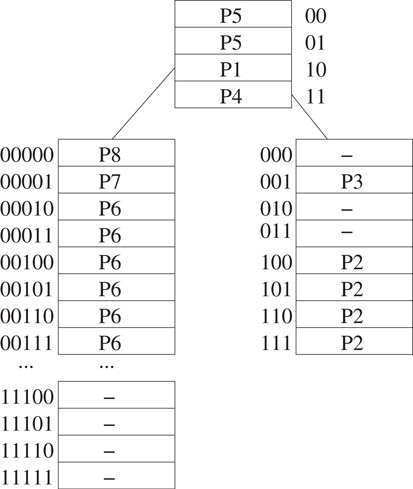
Figure 49.5Two-level VST for prefixes of Figure 49.3a.

Since FSTs are a special case of VSTs, the memory required by the best VST for a given prefix set P and number of expansion levels k is less than or equal to that required by the best FST for P and k. Despite this, FSTs may be preferred in certain router applications “because of their simplicity and slightly faster search time” [7].

Let r-VST be a VST that has at most r levels. Let Opt(N, r) be the cost (i.e., memory requirement) of the best r-VST for a 1-bit trie whose root is N. Nilsson and Karlsson [16] propose a greedy heuristic to construct optimal VSTs. The resulting VSTs are known as LC-tries (level-compressed tries) and were first proposed in a more general context by Andersson and Nilsson [17]. An LC-tries obtained from a 1-bit trie by replacing full subtries of the 1-bit trie by single multibit nodes. This replacement is done by examining the 1-bit trie top to bottom (i.e., from root to leaves). Srinivasan and Varghese [7], have obtained the following dynamic programming recurrence for Opt(N, r).

$\begin{aligned} O p t (N, r) & = min_{s \in {1 \dots 1 + h e i g h t (N)}} {2^{s} + \sum_{M \in D_{s} (N)} O p t (M, r - 1)}, r > 1 \end{aligned}$ $\begin{aligned} O p t (N, r) & = min_{s \in {1 \dots 1 + h e i g h t (N)}} {2^{s} + \sum_{M \in D_{s} (N)} O p t (M, r - 1)}, r > 1 \end{aligned}$	(49.3)

where D_s(N) is the set of all descendants of N that are at level s of N. For example, D1(N) is the set of children of N and D2(N) is the set of grandchildren of N. height(N) is the maximum level at which the trie rooted at N has a node. For example, in Figure 49.3b, the height of the trie rooted at N1 is 5. When r = 1,

$O p t (N, 1) = 2^{1 + h e i g h t (N)}$ $O p t (N, 1) = 2^{1 + h e i g h t (N)}$	(49.4)

Srinivasan and Varghese [7], describe a way to determine Opt(R, k) using Equations 49.4 and 49.5. The complexity of their algorithm is O(p * W * k), where p is the number of nodes in the 1-bit trie for the prefixes (p = O(n) for realistic router tables). Sahni and Kim [18] provide an alternative way to compute Opt(R, k) in O(pWk) time. The algorithm of [18], however, performs fewer operations and has fewer cache misses. When the cost of operations dominates the run time, the algorithm of [18] is expected to be about 6 times as fast as that of [7] (for available router databases). When cache miss time dominates the run time, the algorithm of [18] could be 12 times as fast when k = 2 and 42 times as fast when k = 7.

We describe the formulation used in Reference 18. Let

O p t (N, s, r) = \sum_{M \in D_{s} (N)} O p t (M, r), s > 0, r > 1,

$O p t (N, s, r) = \sum_{M \in D_{s} (N)} O p t (M, r), s > 0, r > 1,$

and let Opt(N, 0, r) = Opt(N, r). From Equations 49.4 and 49.5, it follows that:

$\begin{aligned} O p t (N, 0, r) & = m i n_{s \in {1 \dots 1 + h e i g h t (N)}} {2^{s} + O p t (N, s, r - 1)}, r > 1 \end{aligned}$ $\begin{aligned} O p t (N, 0, r) & = m i n_{s \in {1 \dots 1 + h e i g h t (N)}} {2^{s} + O p t (N, s, r - 1)}, r > 1 \end{aligned}$	(49.5)

and

$O p t (N, 0, 1) = 2^{1 + h e i g h t (N)} .$ $O p t (N, 0, 1) = 2^{1 + h e i g h t (N)} .$	(49.6)

For s > 0 and r > 1, we get

$\begin{matrix} O p t (N, s, r) & = & \sum_{M \in D_{s} (N)} O p t (M, r) \\ = & O p t (L e f t C h i l d (N), s - 1, r) \\ + O p t (R i g h t C h i l d (N), s - 1, r) . \end{matrix}$ $\begin{matrix} O p t (N, s, r) & = & \sum_{M \in D_{s} (N)} O p t (M, r) \\ = & O p t (L e f t C h i l d (N), s - 1, r) \\ + O p t (R i g h t C h i l d (N), s - 1, r) . \end{matrix}$	(49.7)

For Equation 49.9, we need the following initial condition:

$O p t (n u l l,^{},^{}) = 0$ $O p t (n u l l,^{},^{}) = 0$	(49.8)

With the assumption that the number of nodes in the 1-bit trie is O(n), we see that the number of Opt(* , * , * ) values is O(nWk). Each Opt( * , * , * ) value may be computed in O(1) time using Equations 49.7 through 49.11 provided the Opt values are computed in postorder. Therefore, we may compute Opt(R, k) = Opt(R, 0, k) in O(pWk) time. The algorithm of [18] requires O(W2k) memory for the Opt( * , * , * ) values. To see this, notice that there can be at most W + 1 nodes N whose Opt(N, * , * ) values must be retained at any given time, and for each of these at most W + 1 nodes, O(Wk) Opt(N, * , * ) values must be retained. To determine the optimal strides, each node of the 1-bit trie must store the stride s that minimizes the right side of Equation 49.7 for each value of r. For this purpose, each 1-bit trie node needs O(k) space. Since the 1-bit trie has O(n) nodes in practice, the memory requirements of the 1-bit trie are O(nk). The total memory required is, therefore, O(nk + W2k).

In practice, we may prefer an implementation that uses considerably more memory. If we associate a cost array with each of the p nodes of the 1-bit trie, the memory requirement increases to O(pWk). The advantage of this increased memory implementation is that the optimal strides can be recomputed in O(W2k) time (rather than O(pWk)) following each insert or delete of a prefix. This is so because, the Opt(N, * , * ) values need be recomputed only for nodes along the insert/delete path of the 1-bit trie. There are O(W) such nodes.

Faster algorithms to determine optimal 2- and 3-VSTs also are developed in Reference 18.

49.2.5Binary Search Trees

Sahni and Kim [19] propose the use of a collection of red-black trees (see Chapter 11) to determine LMP(d). The CRBT comprises a front-end data structure that is called the binary interval tree (BIT) and a back-end data structure called a collection of prefix trees (CPT). For any destination address d, define the matching basic interval to be a basic interval with the property that r_i ≤ d ≤ r_i+1 (note that some ds have two matching basic intervals).

The BIT is a binary search tree that is used to search for a matching basic interval for d. The BIT comprises internal and external nodes and there is one internal node for each r_i. Since the BIT has q internal nodes, it has q + 1 external nodes. The first and last of these, in inorder, have no significance. The remaining q − 1 external nodes, in inorder, represent the q − 1 basic intervals of the given prefix set. Figure 49.6a gives a possible (we say possible because, any red-black binary search tree organization for the internal nodes will suﬃce) BIT for our five-prefix example of Figure 49.2a. Internal nodes are shown as rectangles while circles denote external nodes. Every external node has three pointers: startPointer, finishPointer, and basicIntervalPointer. For an external node that represents the basic interval [r_i, r_i+1], startPointer (finishPointer) points to the header node of the prefix tree (in the back-end structure) for the prefix (if any) whose range start and finish points are r_i (r_i+1). Note that only prefixes whose length is W can have this property. basicIntervalPointer points to a prefix node in a prefix tree of the back-end structure. In Figure 49.6a, the labels in the external (circular) nodes identify the represented basic interval. The external node with r1 in it, for example, has a basicIntervalPointer to the rectangular node labeled r1 in the prefix tree of Figure 49.6b.

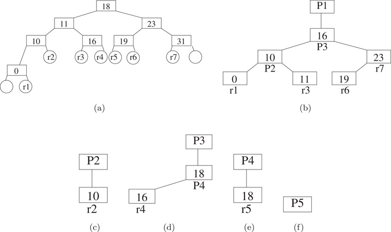
Figure 49.6CBST for Figure 49.2a. (a) base interval tree (b) prefix tree for P1 (c) prefix tree for P2 (d) prefix tree for P3 (e) prefix tree for P4 (f) prefix tree for P5.

For each prefix and basic interval, x, define next(x) to be the smallest range prefix (i.e., the longest prefix) whose range includes the range of x. For the example of Figure 49.2a, the next() values for the basic intervals r1 through r7 are, respectively, P1, P2, P1, P3, P4, P1, and P1. Notice that the next value for the range [r_i, r_i+1] is the same as the “> ” value for r_i in Figure 49.2b, 1 ≤ i < q. The next() values for the nontrivial prefixes P1 through P4 of Figure 49.2a are, respectively, “-,” P1, P1, and P3.

The back-end structure, which is a collection of prefix trees (CPT), has one prefix tree for each of the prefixes in the router table. Each prefix tree is a red-black tree. The prefix tree for prefix P comprises a header node plus one node, called a prefix node, for every nontrivial prefix or basic interval x such that next(x) = P. The header node identifies the prefix P for which this is the prefix tree. The prefix trees for each of the five prefixes of Figure 49.2a are shown in Figure 49.6b–f. Notice that prefix trees do not have external nodes and that the prefix nodes of a prefix tree store the start point of the range or prefix represented by that prefix node. In the figures, the start points of the basic intervals and prefixes are shown inside the prefix nodes while the basic interval or prefix name is shown outside the node.

The search for LMP(d) begins with a search of the BIT for the matching basic interval for d. Suppose that external node Q of the BIT represents this matching basic interval. When the destination address equals the left (right) end-point of the matching basic interval and startPointer (finishPointer) is not null, LMP(d) is pointed to by startPointer (finishPointer). Otherwise, the back-end CPT is searched for LMP(d). The search of the back-end structure begins at the node Q.basicIntervalPointer. By following parent pointers from Q.basicIntervalPointer, we reach the header node of the prefix tree that corresponds to LMP(d).

When a CRBT is used, LMP(d) may be found in O(log n) time. Inserts and deletes also take O(log n) time when a CRBT is used. In Reference 20, Sahni and Kim propose an alternative BIT structure (ABIT) that has internal nodes only. Although the ABIT structure increases the memory requirements of the router table, the time to search, insert, and delete is reduced by a constant factor [20]. Suri et al. [21] have proposed a B-tree data structure for dynamic router tables. Using their structure, we may find the longest matching prefix in O(log n) time. However, inserts/deletes take O(W log n) time. The number of cache misses is O(log n) for each operation. When W bits fit in O(1) words (as is the case for IPv4 and IPv6 prefixes) logical operations on W-bit vectors can be done in O(1) time each. In this case, the scheme of [21] takes O(log W * log n) time for an insert and O(W + log n) = O(W) time for a delete. An alternative B-tree router-table design has been proposed by Lu and Sahni [22]. Although the asymptotic complexity of each of the router-table operations is the same using either B-tree router-table design, the design of Lu and Sahni [22] has fewer cache misses for inserts and deletes; the number of cache misses when searching for lmp(d) is the same using either design. Consequently, inserts and deletes are faster when the design of Lu and Sahni [22] is used.

Several researchers ([20,23–25], for example), have investigated router table data structures that account for bias in access patterns. Gupta, Prabhakar, and Boyd [25], for example, propose the use of ranges. They assume that access frequencies for the ranges are known, and they construct a bounded-height binary search tree of ranges. This binary search tree accounts for the known range access frequencies to obtain near-optimal IP lookup. Although the scheme of [25] performs IP lookup in near-optimal time, changes in the access frequencies, or the insertion or removal of a prefix require us to reconstruct the data structure, a task that takes O(n log n) time.

Ergun et al. [24] use ranges to develop a biased skip list structure that performs longest prefix-matching in O(log n) expected time. Their scheme is designed to give good expected performance for bursty^* access patterns.” The biased skip list scheme of Ergun et al. [24] permits inserts and deletes in O(log n) time only in the severely restricted and impractical situation when all prefixes in the router table are of the same length. For the more general, and practical, case when the router table comprises prefixes of different length, their scheme takes O(n) expected time for each insert and delete. Sahni and Kim [20] extend the biased skip lists of Ergun et al. [24] to obtain a biased skip lists structure in which longest prefix-matching as well as inserts and deletes take O(log n) expected time. They also propose a splay tree scheme (see Chapter 13) for bursty access patterns. In this scheme, longest prefix-matching, insert and delete have an O(log n) amortized complexity.

49.2.6Priority Search Trees

A priority-search tree (PST) [28] (see Chapter 19) is a data structure that is used to represent a set of tuples of the form (key1, key2, data), where key1 ≥ 0, key2 ≥ 0, and no two tuples have the same key1 value. The data structure is simultaneously a min-tree on key2 (i.e., the key2 value in each node of the tree is ≤ the key2 value in each descendant node) and a search tree on key1. There are two common PST representations [28]:

1.In a radix priority-search tree (RPST), the underlying tree is a binary radix tree on key1.

2.In a red-black priority-search tree (RBPST), the underlying tree is a red-black tree.

McCreight [28] has suggested a PST representation of a collection of ranges with distinct finish points. This representation uses the following mapping of a range r into a PST tuple:

$(k e y 1, k e y 2, d a t a) = (f i n i s h (r), s t a r t (r), d a t a)$ $(k e y 1, k e y 2, d a t a) = (f i n i s h (r), s t a r t (r), d a t a)$	(49.9)

where data is any information (e.g., next hop) associated with the range. Each range r is, therefore mapped to a point map1(r) = (x, y) = (key1, key2) = (finish(r), start(r)) in 2-dimensional space.

Let ranges(d) be the set of ranges that match d. McCreight [28] has observed that when the mapping of Equation 49.12 is used to obtain a point set P = map1(R) from a range set R, then ranges(d) is given by the points that lie in the rectangle (including points on the boundary) defined by x_left = d, x_right = ∞, y_top = d, and y_bottom = 0. These points are obtained using the method $e n u m e r a t e R e c t a n g l e (x_{l e f t}, x_{r i g h t}, y_{t o p})$ $e n u m e r a t e R e c t a n g l e (x_{l e f t}, x_{r i g h t}, y_{t o p})$ = enumerateRectangle(d, ∞, d) of a PST (y_bottom is implicit and is always 0).

When an RPST is used to represent the point set P, the complexity of

e n u m e r a t e R e c t a n g l e (x_{l e f t}, x_{r i g h t}, y_{t o p})

$e n u m e r a t e R e c t a n g l e (x_{l e f t}, x_{r i g h t}, y_{t o p})$

is O(log maxX + s), where maxX is the largest x value in P and s is the number of points in the query rectangle. When the point set is represented as an RBPST, this complexity becomes O(log n + s), where n = |P|. A point (x, y) (and hence a range [y, x]) may be inserted into or deleted from an RPST (RBPST) in O(log maxX) (O(log n)) time [28].

Let R be a set of prefix ranges. For simplicity, assume that R includes the range that corresponds to the prefix *. With this assumption, LMP(d) is defined for every d. One may verify that LMP(d) is the prefix whose range is

[m a x S t a r t (r a n g e s (d)), m i n F i n i s h (r a n g e s (d))] .

$[m a x S t a r t (r a n g e s (d)), m i n F i n i s h (r a n g e s (d))] .$

Lu and Sahni [29] show that R must contain such range. To find this range easily, we first transform P = map1(R) into a point set transform1(P) so that no two points of transform1(P) have the same x-value. Then, we represent transform1(P) as a PST. For every (x, y) ∈ P, define transform1(x, y) = (x′, y′) = (2Wx − y + 2W − 1, y). Then, transform1(P) = {transform1(x, y)|(x, y) ∈ P}.

We see that 0 ≤ x′ < 2^2W for every (x′, y′) ∈ transform1(P) and that no two points in transform1(P) have the same x′-value. Let PST1(P) be the PST for transform1(P). The operation

e n u m e r a t e R e c t a n g l e (2^{W} d - d + 2^{W} - 1, \infty, d)

$e n u m e r a t e R e c t a n g l e (2^{W} d - d + 2^{W} - 1, \infty, d)$

performed on PST1 yields ranges(d). To find LMP(d), we employ the

m i n X i n R e c t a n g l e (x_{l e f t}, x_{r i g h t}, y_{t o p})

$m i n X i n R e c t a n g l e (x_{l e f t}, x_{r i g h t}, y_{t o p})$

operation, which determines the point in the defined rectangle that has the least x-value. It is easy to see that

m i n X i n R e c t a n g l e (2^{W} d - d + 2^{W} - 1, \infty, d)

$m i n X i n R e c t a n g l e (2^{W} d - d + 2^{W} - 1, \infty, d)$

performed on PST1 yields LMP(d).

To insert the prefix whose range in [u, v], we insert transform1(map1([u, v])) into PST1. In case this prefix is already in PST1, we simply update the next-hop information for this prefix. To delete the prefix whose range is [u, v], we delete transform1(map1([u, v])) from PST1. When deleting a prefix, we must take care not to delete the prefix *. Requests to delete this prefix should simply result in setting the next-hop associated with this prefix to ∅.

Since, minXinRectangle, insert, and delete each take O(W) (O(log n)) time when PST1 is an RPST (RBPST), PST1 provides a router-table representation in which longest-prefix matching, prefix insertion, and prefix deletion can be done in O(W) time each when an RPST is used and in O(log n) time each when an RBPST is used.

Tables 49.1 and 49.2 summarize the performance characteristics of various data structures for the longest matching-prefix problem.

Table 49.1Time Complexity of Data Structures for Longest Matching-Prefix

Data Structure	Search	Update
Linear List	O(n)	O(n)
End-point Array	O(log n)	O(n)
Sets of Equal-Length Prefixes	O(α + log W) expected	$O (α \sqrt[α]{n} W \log W)$ $O (α \sqrt[α]{n} W \log W)$ expected
1-bit tries	O(W)	O(W)
s-bit Tries	O(W/s)	-
CRBT	O(log n)	O(log n)
ACRBT	O(log n)	O(log n)
BSLPT	O(log n) expected	O(log n) expected
CST	O(log n) amortized	O(log n) amortized
PST	O(log n)	O(log n)

Table 49.2Memory Complexity of Data Structures for Longest Matching-Prefix

Data Structure	Memory Usage
Linear List	O(n)
End-point Array	O(n)
Sets of Equal-Length Prefixes	O(n log W)
1-bit tries	O(nW)
s-bit Tries	O(2snW/s)
CRBT	O(n)
ACRBT	O(n)
BSLPT	O(n)
CST	O(n)
PST	O(n)

49.3Highest-Priority Matching

The trie data structure may be used to represent a dynamic prefix-router-table in which the highest-priority tie-breaker is in use. Using such a structure, each of the dynamic router-table operations may be performed in O(W) time. Lu and Sahni [30] have developed the binary tree on binary tree (BOB) data structure for highest-priority dynamic router-tables. Using BOB, a lookup takes O(log2n) time and cache misses; a new rule may be inserted and an old one deleted in O(log n) time and cache misses. Although BOB handles filters that are non-intersecting ranges, specialized versions of BOB have been proposed for prefix filters. Using the data structure PBOB (prefix BOB), a lookup, rule insertion and deletion each take O(W) time and cache misses. The data structure LMPBOB (longest matching-prefix BOB) is proposed in Reference 30 for dynamic prefix-router-tables that use the longest matching-prefix rule. Using LMPBOB, the longest matching-prefix may be found in O(W) time and O(log n) cache misses; rule insertion and deletion each take O(log n) time and cache misses. On practical rule tables, BOB and PBOB perform each of the three dynamic-table operations in O(log n) time and with O(log n) cache misses. Other data structures for maximum-priority matching are developed in References 31 and 32.

49.3.1The Data Structure BOB

The data structure binary tree on binary tree (BOB) comprises a single balanced binary search tree at the top level. This top-level balanced binary search tree is called the point search tree (PTST). For an n-rule NHRT, the PTST has at most 2n nodes (we call this the PTST size constraint). With each node z of the PTST, we associate a point, point(z). The PTST is a standard red-black binary search tree (actually, any binary search tree structure that supports efficient search, insert, and delete may be used) on the point(z) values of its node set [1]. That is, for every node z of the PTST, nodes in the left subtree of z have smaller point values than point(z), and nodes in the right subtree of z have larger point values than point(z).

Let R be the set of nonintersecting ranges. Each range of R is stored in exactly one of the nodes of the PTST. More specifically, the root of the PTST stores all ranges r ∈ R such that start(r) ≤ point(root) ≤ finish(r); all ranges r ∈ R such that finish(r) < point(root) are stored in the left subtree of the root; all ranges r ∈ R such that point(root) < start(r) (i.e., the remaining ranges of R) are stored in the right subtree of the root. The ranges allocated to the left and right subtrees of the root are allocated to nodes in these subtrees using the just stated range allocation rule recursively.

For the range allocation rule to successfully allocate all r ∈ R to exactly one node of the PTST, the PTST must have at least one node z for which start(r) ≤ point(z) ≤ finish(r). Figure 49.7 gives an example set of nonintersecting ranges and a possible PTST for this set of ranges (we say possible, because we haven’t specified how to select the point(z) values and even with specified point(z) values, the corresponding red-black tree isn’t unique). The number inside each node is point(z), and outside each node, we give ranges(z).

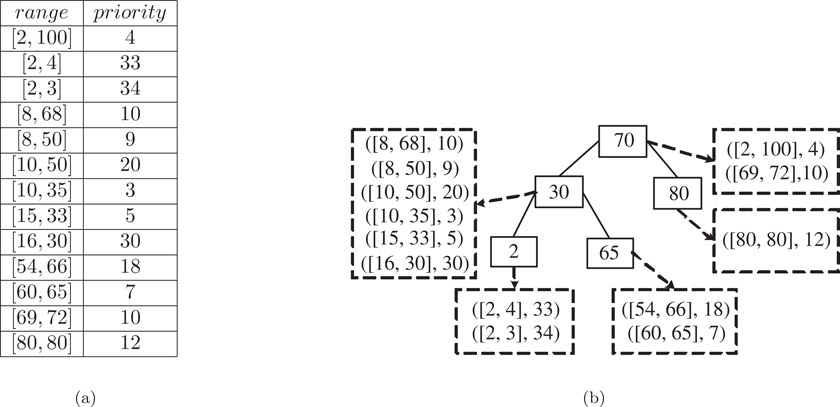
Figure 49.7(a) A nonintersecting range set and (b) A possible PTST.

Let ranges(z) be the subset of ranges of R allocated to node z of the PTST.^* Since the PTST may have as many as 2n nodes and since each range of R is in exactly one of the sets ranges(z), some of the ranges(z) sets may be empty.

The ranges in ranges(z) may be ordered using the < relation for non-intersecting ranges.^† Using this < relation, we put the ranges of ranges(z) into a red-black tree (any balanced binary search tree structure that supports efficient search, insert, delete, join, and split may be used) called the range search-tree or RST(z). Each node x of RST(z) stores exactly one range of ranges(z). We refer to this range as range(x). Every node y in the left (right) subtree of node x of RST(z) has range(y) < range(x) (range(y) > range(x)). In addition, each node x stores the quantity mp(x), which is the maximum of the priorities of the ranges associated with the nodes in the subtree rooted at x. mp(x) may be defined recursively as below.

m p (x) = {\begin{cases} p (x) & if x is leaf \\ max {m p (l e f t C h i l d (x)), m p (r i g h t C h i l d (x)), p (x)} & otherwise \end{cases}

$m p (x) = {\begin{cases} p (x) & if x is leaf \\ max {m p (l e f t C h i l d (x)), m p (r i g h t C h i l d (x)), p (x)} & otherwise \end{cases}$

where p(x) = priority(range(x)). Figure 49.8 gives a possible RST structure for ranges(30) of Figure 49.7b.

Figure 49.8An example RST for ranges(30) of Figure 49.7b. Each node shows (range(x), p(x), mp(x)).

Lemma 49.1

(Lu and Sahni [30])Let z be a node in a PTST and let x be a node in RST(z). Let st(x) = start(range(x)) and fn(x) = finish(range(x)).

1.For every node y in the right subtree of x, st(y) ≥ st(x) and fn(y) ≤ fn(x).

2.For every node y in the left subtree of x, st(y) ≤ st(x) and fn(y) ≥ fn(x).

Both BOB and BOT (the binary tree on trie structure of Gupta and McKeown [32]) use a range allocation rule identical to that used in an interval tree [33] (See Chapter 19). While BOT may be used with any set of ranges, BOB applies only to a set of non-intersecting ranges. However, BOB reduces the search complexity of BOT from O(W log n) to O(log2n) and reduces the update complexity from O(W) to O(log n).

49.3.2Search for the Highest-Priority Matching Range

The highest-priority range that matches the destination address d may be found by following a path from the root of the PTST toward a leaf of the PTST. Figure 49.9 gives the algorithm. For simplicity, this algorithm finds hp = priority(hpr(d)) rather than hpr(d). The algorithm is easily modified to return hpr(d) instead.

Figure 49.9Algorithm to find priority(hpr(d)).

We begin by initializing hp = − 1 and z is set to the root of the PTST. This initialization assumes that all priorities are ≥ 0. The variable z is used to follow a path from the root toward a leaf. When d > point(z), d may be matched only by ranges in RST(z) and those in the right subtree of z. The method RST(z)->hpRight(d,hp) (Figure 49.10) updates hp to reflect any matching ranges in RST(z). This method makes use of the fact that d > point(z). Consider a node x of RST(z). If d > fn(x), then d is to the right (i.e., d > finish(range(x))) of range(x) and also to the right of all ranges in the right subtree of x. Hence, we may proceed to examine the ranges in the left subtree of x. When d ≤ fn(x), range(x) as well as all ranges in the left subtree of x match d. Additional matching ranges may be present in the right subtree of x. hpLeft(d, hp) is the analogous method for the case when d < point(z).

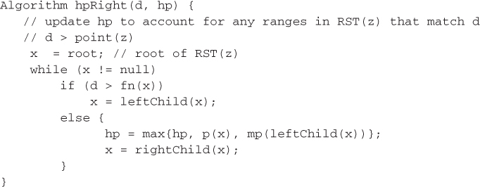
Figure 49.10Algorithm hpRight(d, hp).

Complexity The complexity of the invocation RST(z)->hpRight(d,hp) is readily seen to be O(height(RST(z)) = O(log n). Consequently, the complexity of hp(d) is O(log2n). To determine hpr(d) we need only add code to the methods hp(d), hpRight(d, hp), and hpLeft(d, hp) so as to keep track of the range whose priority is the current value of hp. So, hpr(d) may be found in O(log2n) time also.

The details of the insert and delete operation as well of the BOB variants PBOB and LMPBOB may be found in Reference 30.

49.4Most-Specific-Range Matching

Let msr(d) be the most-specific range that matches the destination address d. For static tables, we may simply represent the n ranges by the up to 2n − 1 basic intervals they induce. For each basic interval, we determine the most-specific range that matches all points in the interval. These up to 2n − 1 basic intervals may then be represented as up to 4n − 2 prefixes [31] with the property that msr(d) is uniquely determined by LMP(d). Now, we may use any of the earlier discussed data structures for static tables in which the filters are prefixes. In this section, therefore, we discuss only those data structures that are suitable for dynamic tables.

49.4.1Nonintersecting Ranges

Let R be a set of nonintersecting ranges. For simplicity, assume that R includes the range z that matches all destination addresses (z = [0, 232 − 1] in the case of IPv4). With this assumption, msr(d) is defined for every d. Similar to the case of prefixes, for nonintersecting ranges, msr(d) is the range [maxStart(ranges(d)), minFinish(ranges(d))] (Lu and Sahni [29] show that R must contain such a range). We may use

P S T 1 (t r a n s f o r m 1 (m a p 1 (R)))

$P S T 1 (t r a n s f o r m 1 (m a p 1 (R)))$

to find msr(d) using the same method described in Section 49.2.6 to find LMP(d).

Insertion of a range r is to be permitted only if r does not intersect any of the ranges of R. Once we have verified this, we can insert r into PST1 as described in Section 49.2.6. Range intersection may be verified by noting that there are two cases for range intersection. When inserting r = [u, v], we need to determine if ∃s = [x, y] ∈ R[u < x ≤ v < y∨x < u ≤ y < v]. We see that ∃s ∈ R[x < u ≤ y < v] iff map1(R) has at least one point in the rectangle defined by x_left = u, x_right = v − 1, and y_top = u − 1 (recall that y_bottom = 0 by default). Hence, ∃s ∈ R[x < u ≤ y < v] iff minXinRectangle(2Wu − (u − 1) + 2W − 1, 2W(v − 1) + 2W − 1, u − 1) exists in PST1.

To verify ∃s ∈ R[u < x ≤ v < y], map the ranges of R into 2-dimensional points using the mapping, map2(r) = (start(r), 2W − 1 − finish(r)). Call the resulting set of mapped points map2(R). We see that ∃s ∈ R[u < x ≤ v < y] iff map2(R) has at least one point in the rectangle defined by x_left = u + 1, x_right = v, and y_top = (2W − 1) − v − 1. To verify this, we maintain a second PST, PST2 of points in transform2(map2(R)), where transform2(x, y) = (2Wx + y, y) Hence, ∃s ∈ R[u < x ≤ v < y] iff minXinRectangle(2W(u + 1), 2Wv + (2W − 1) − v − 1, (2W − 1) − v − 1) exists.

To delete a range r, we must delete r from both PST1 and PST2. Deletion of a range from a PST is similar to deletion of a prefix as discussed in Section 49.2.6.

The complexity of the operations to find msr(d), insert a range, and delete a range are the same as that for these operations for the case when R is a set of ranges that correspond to prefixes.

49.4.2Conflict-Free Ranges

The range set R has a conflict iff there exists a destination address d for which ranges(d) ≠ ∅ ∧ msr(d) = ∅. R is conflict free iff it has no conflict. Notice that sets of prefix ranges and sets of nonintersecting ranges are conflict free. The two-PST data structure of Section 49.4.1 may be extended to the general case when R is an arbitrary conflict-free range set. Once again, we assume that R includes the range z that matches all destination addresses. PST1 and PST2 are defined for the range set R as in Sections 49.2.6 and 49.4.1.

Lu and Sahni [29] have shown that when R is conflict free, msr(d) is the range

[m a x S t a r t (r a n g e s (d)), m i n F i n i s h (r a n g e s (d))]

$[m a x S t a r t (r a n g e s (d)), m i n F i n i s h (r a n g e s (d))]$

Hence, msr(d) may be obtained by performing the operation

m i n X i n R e c t a n g l e (2^{W} d - d + 2^{W} - 1, \infty, d)

$m i n X i n R e c t a n g l e (2^{W} d - d + 2^{W} - 1, \infty, d)$

on PST1. Insertion and deletion are complicated by the need to verify that the addition or deletion of a range to/from a conflict-free range set leaves behind a conflict-free range set. To perform this check efficiently, Lu and Sahni [29] augment PST1 and PST with a representation for the chains in the normalized range-set, norm(R), that corresponds to R. This requires the use of several red-black trees. The reader is referred to [29] for a description of this augmentation.

The overall complexity of the augmented data structure of [29] is O(log n) for each operation when RBPSTs are used for PST1 and PST2. When RPSTs are used, the search complexity is O(W) and the insert and delete complexity is O(W + log n) = O(W).

Acknowledgments

This work was supported, in part, by the National Science Foundation under grant CCR-9912395.

References

1.E. Horowitz, S. Sahni, and D. Mehta, Fundamentals of data structures in C++, W.H. Freeman, NY, 1995, 653 pages.

2.D. Shah and P. Gupta, Fast updating algorithms for TCAMs, IEEE Micro, 21, 1, 36–47, 2002.

3.F. Zane, G. Narlikar, and A. Basu, CoolCAMs: Power-efficient TCAMs for forwarding engines, IEEE INFOCOM, 2003.

4.F. Baboescu, S. Singh, and G. Varghese, Packet classification for core routers: Is there an alternative to CAMs?, IEEE INFOCOM, 2003.

5.B. Lampson, V. Srinivasan, and G. Varghese, IP lookup using multi-way and multicolumn search, IEEE INFOCOM, 1998.

6.M. Waldvogel, G. Varghese, J. Turner, and B. Plattner, Scalable high speed IP routing lookups, ACM SIGCOMM, 25–36, 1997.

7.V. Srinivasan and G. Varghese, Faster IP lookups using controlled prefix expansion, ACM Transactions on Computer Systems, Feb:1–40, 1999.

8.V. Srinivasan, Fast and efficient Internet lookups, CS Ph.D Dissertation, Washington University, Aug., 1999.

9.K. Kim and S. Sahni, IP lookup by binary search on length, Journal of Interconnection Networks, 3, 3&4, 105–128, 2002.

10.M. Berg, M. Kreveld, and J. Snoeyink, Two- and three-dimensional point location in rectangular subdivisions, Journal of Algorithms, 18, 2, 256–277, 1995.

11.D. E. Willard, Log-logarithmic worst-case range queries are possible in space θ(N), Information Processing Letters, 17, 81–84, 1983.

12.P. V. Emde Boas, R. Kass, and E. Zijlstra, Design and implementation of an efficient priority queue, Mathematical Systems Theory, 10, 99–127, 1977.

13.S. Sahni and K. Kim, Efficient construction of fixed-stride multibit tries for IP lookup, Proceedings 8th IEEE Workshop on Future Trends of Distributed Computing Systems, 2001.

14.M. Degermark, A. Brodnik, S. Carlsson, and S. Pink, Small forwarding tables for fast routing lookups, ACM SIGCOMM, 3–14, 1997.

15.A. Basu and G. Narlikar, Fast incremental updates for pipelined forwarding engines, IEEE INFOCOM, 2003.

16.S. Nilsson and G. Karlsson, Fast address look-up for Internet routers, IEEE Broadband Communications, 1998.

17.A. Andersson and S. Nillson, Improved behavior of tries by adaptive branching, Information Processing Letters, 46, 295–300, 1993.

18.S. Sahni and K. Kim, Efficient construction of variable-stride multibit tries for IP lookup, Proceedings IEEE Symposium on Applications and the Internet (SAINT), 220–227, 2002.

19.S. Sahni and K. Kim, O(log n) dynamic packet routing, IEEE Symposium on Computers and Communications, 443–448, 2002.

20.S. Sahni and K. Kim, Efficient dynamic lookup for bursty access patterns, submitted.

21.S. Suri, G. Varghese, and P. Warkhede, Multiway range trees: Scalable IP lookup with fast updates, GLOBECOM, 2001.

22.H. Lu and S. Sahni, A B-tree dynamic router-table design: Submitted.

23.G. Cheung and S. McCanne, Optimal routing table design for IP address lookups under memory constraints, IEEE INFOCOM, 1999.

24.F. Ergun, S. Mittra, S. Sahinalp, J. Sharp, and R. Sinha, A dynamic lookup scheme for bursty access patterns, IEEE INFOCOM, 2001.

25.P. Gupta, B. Prabhakar, and S. Boyd, Near-optimal routing lookups with bounded worst case performance, IEEE INFOCOM, 2000.

26.K. Claffy, H. Braun, and G Polyzos, A parameterizable methodology for internet traffic flow profiling, IEEE Journal of Selected Areas in Communications, 1995.

27.S. Lin and N. McKeown, A simulation study of IP switching, IEEE INFOCOM, 2000.

28.E. McCreight, Priority search trees, SIAM Jr. on Computing, 14, 1, 257–276, 1985.

29.H. Lu and S. Sahni, O(log n) dynamic router-tables for prefixes and ranges: Submitted.

30.H. Lu and S. Sahni, Dynamic IP router-tables using highest-priority matching: Submitted.

31.A. Feldman and S. Muthukrishnan, Tradeoffs for packet classification, IEEE INFOCOM, 2000.

32.P. Gupta and N. McKeown, Dynamic algorithms with worst-case performance for packet classification, IFIP Networking, 2000.

33.M. deBerg, M. vanKreveld, and M. Overmars, Computational Geometry: Algorithms and Applications, Second Edition, Springer Verlag, 1997.

34.W. Doeringer, G. Karjoth, and M. Nassehi, Routing on longest-matching prefixes, IEEE/ACM Transactions on Networking, 4, 1, 86–97, 1996.

^*This chapter has been reprinted from first edition of this Handbook, without any content updates.

^†We have used this author's affiliation from the first edition of this handbook, but note that this may have changed since then.

^‡A flow is a set of packets that are to be treated similarly for routing purposes.

^*Two ranges [u, v] and [x, y] intersect iff u < x ≤ v < y∨ x < u ≤ y < v.

^*The length of a prefix is the number of bits in that prefix (note that the * is not used in determining prefix length). The length of P1 is 0 and that of P2 is 4.

^†More precisely, W may be defined to be the number of different prefix lengths in the table.

^*When searching S_i, only the first i bits of d are used, because all prefixes in S_i have exactly i bits.

^*Level numbers are assigned beginning with 0 for the root level.

^*In a bursty access pattern the number of different destination addresses in any subsequence of q packets is < < q. That is, if the destination of the current packet is d, there is a high probability that d is also the destination for one or more of the next few packets. The fact that Internet packets tend to be bursty has been noted in References 26 and 27, for example.

^*We have overloaded the function ranges. When u is a node, ranges(u) refers to the ranges stored in node u of a PTST; when u is a destination address, ranges(u) refers to the ranges that match u.

^†Let r and s be two ranges. r < s⇔start(r) < start(s)∨(start(r) = start(s)∧finish(r) > finish(s)).

..................Content has been hidden....................

You can't read the all page of ebook, please click here login for view all page.

Table of Contents for 49. IP Router Tables

Create new playlist

Sign In

Sign Up

Table of Contents for
49. IP Router Tables