59. Computational Biology

In the last 20 years, biological sequence data have been accumulating at exponential rate under continuous improvement of sequencing technology, progress in computer science, and steady increase of funding. Molecular sequence databases (e.g., EMBL, Genbank, DDJB, Entrez, Swissprot, etc.) currently collect hundreds of thousands of sequences of nucleotides and amino acids from biological laboratories all over the world, reaching into the hundreds of terabytes. Such an exponential growth makes it increasingly important to have fast and automatic methods to process, analyze, and visualize massive amounts of data.

The exploration of many computational problems arising in contemporary molecular biology has now grown to become a mature field of computer science. A coarse selection would include sequence homology and alignment, physical and genetic mapping, protein folding and structure prediction, gene‐expression analysis, evolutionary tree construction, gene finding, assembly for shotgun sequencing, gene rearrangements and pattern discovery, among others.

In this chapter, we focus the attention on the applications of suffix trees and suffix arrays to computational biology. In fact, suffix trees, suffix arrays, and their variants are among the most used (and useful) data structures in computational biology. (See Chapters 30 and 31 for more on suffix trees and DAWGs.)

This chapter is divided into three sections. In Sections 59.2 and 59.3, we describe two distinct applications of suffix trees to computational biology. In the first application, the use of suffix trees and DAWGs is essential in developing a linear-time algorithm for solving a pattern discovery problem. In the second application, suffix trees are used to solve a challenging algorithmic problem: the alignment of two or more complete genomes.

In Section 59.4, we describe the FM-index which is a sort of “compressed” suffix array based on a fascinating mathematical transformation called the Burrows–Wheeler transform. Because of its reduced space occupancy, the FM-index for a mammalian genome can be stored entirely in primary memory. Due to its memory efficiency, this data structure is a cornerstone of the majority of alignment tools, as well some assembly tools.

59.2Discovering Unusual Words

In the context of computational biology, “pattern discovery” refers to the automatic identification of biologically significant patterns (or motifs) by statistical methods. These methods originated from the work of R. Staden [1] and have been recently expanded in a subfield of data mining. The underlying assumption is that biologically significant words show distinctive distributional patterns within the genomes of various organisms, and therefore they can be distinguished from the others. The reality is not too far from this hypothesis [2–10], because during the evolutionary process, living organisms have accumulated certain biases toward or against some specific motifs in their genomes. For instance, highly recurring oligonucleotides are often found in correspondence to regulatory regions or protein binding sites of genes [11–14]. Vice versa, rare oligonucleotide motifs may be discriminated against due to structural constraints of genomes or specific reservations for global transcription controls [9,15]. In some prokaryotes, rare motifs can also corresponds to restriction enzyme sites—bacteria have evolved to avoid those motifs to protect themselves.

From a statistical viewpoint, over- and underrepresented words have been studied quite rigorously (see, e.g., Reference 16 for a review). A substantial corpus of works has been also produced by the scientific community which studies combinatorics on words (see, e.g., References 17 and 18, and references therein). In the application domain, however, the “success story” of pattern discovery has been its ability to find previously unknown regulatory elements in DNA sequences [13,19]. Regulatory elements control the expression (i.e., the amount of mRNA produced) of the genes over time, as the result of different external stimuli to the cell and other metabolic processes that take place internally in the cell. These regulatory elements are typically, but not always, found in the upstream sequence of a gene. The upstream sequence is defined as a portion of DNA of 1–2 k bases of length, located upstream of the site that controls the start of transcription. The regulatory elements correspond to binding sites for the factors involved in the transcriptional process. The complete characterization of these elements is a critical step in understanding the function of different genes and the complex network of interaction between them.

The use of pattern discovery to find regulatory elements relies on a conceptual hypothesis that genes which exhibit similar expression patterns are assumed to be involved in the same biological process or functions. Although many believe that this assumption is an oversimplification, it is still a good working hypothesis. Co-expressed genes are therefore expected to share common regulatory domains in the upstream regions for the coordinated control of gene expression. In order to elucidate genes which are co-expressed as a result of a specific stress or condition, a DNA microarray experiment is typically designed. After collecting data from the microarray, co-expressed genes are usually obtained by clustering the time series corresponding to their expression profiles.

As said, words that occur unexpectedly often or rarely in genetic sequences have been variously linked to biological meanings and functions. With increasing availability of whole genomes, exhaustive statistical tables and global detectors of unusual words on a scale of millions, even billions of bases become conceivable. It is natural to ask how large such tables may grow with increasing length of the input sequence, and how fast they can be computed. These problems need to be regarded not only from the conventional perspective of asymptotic space and time complexities, but also in terms of the volumes of data produced and ultimately, of practical accessibility and usefulness. Tables that are too large at the outset saturate the perceptual bandwidth of the user and might suggest approaches that sacrifice some modeling accuracy in exchange for an increased throughput.

The number of distinct substrings in a string is at worst quadratic in the length of that string. The situation does not improve if one only computes and displays the most unusual words in a given sequence. This presupposes comparing the frequency of occurrence of every word in that sequence with its expectation: a word that departs from expectation beyond some preset threshold will be labeled as unusual or surprising. Departure from expectation is assessed by a distance measure often called a score function. The typical format for a z-score is that of a difference between observed and expected counts, usually normalized to some suitable moment. For most a priori models of a source, it is not difficult to come up with extremal examples of observed sequences in which the number of, say, overrepresented substrings grows itself with the square of the sequence length.

An extensive study of probabilistic models and scores for which the population of potentially unusual words in a sequence can be described by tables of size at worst linear in the length of that sequence was carried out in Reference 20. That study not only leads to more palatable representations for those tables but also supports (nontrivial) linear time and space algorithms for their constructions, as described in what follows. These results do not mean that the number of unusual words must be linear in the input, but just that their representation and detection can be made such. Specifically, it is seen that it suffices to consider as candidate surprising words only the members of an a priori well-identified set of “representative” words, where the cardinality of that set is linear in the text length. By the representatives being identifiable a priori, we mean that they can be known before any score is computed. By neglecting the words other than the representatives we are not ruling out that those words might be surprising. Rather, we maintain that any such word: (i) is embedded in one of the representatives and (ii) does not have a bigger score or degree of surprise than its representative (hence, it would add no information to compute and give its score explicitly).

59.2.1Statistical Analysis of Words

For simplicity of exposition, assume that the source can be modeled by a Bernoulli distribution, that is, symbols are generated i.i.d., and that strings are ranked based on their number of occurrences (possibly overlapping). The results reported in the rest of this section can be extended to other models and counts [20].

We use standard concepts and notation about strings, for which we refer to References 21 and 22. For a substring y of a text x over an alphabet Σ, we denote by f_x(y) the number of occurrences of y in x. We have $f_{x} (y) = | p o s_{x} (y) | = | e n d p o s_{x} (y) |$ $f_{x} (y) = | p o s_{x} (y) | = | e n d p o s_{x} (y) |$ , where pos_x(y) is the start-set of starting positions of y in x and endpos_x(y) is the similarly defined end-set. Clearly, for any extension uyv of y, f_x(uyv) ≤ f_x(y).

Suppose now that string x = x[0]x[1]…x[n − 1] is a realization of a stationary ergodic random process and y = y[0]y[1]…y[m − 1] = y is an arbitrary but fixed pattern over Σ with m < n. We define Z_i, for all i ∈ [0…n − m], to be 1 if y occurs in x starting at position i, 0 otherwise, so that

Z_{y} = \sum_{i = 0}^{n - m} Z_{i}

$Z_{y} = \sum_{i = 0}^{n - m} Z_{i}$

is the random variable for f_x(y).

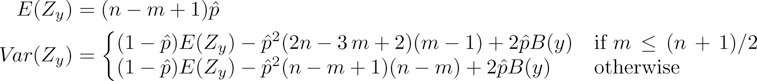
Expressions for the expectation and the variance for the number of occurrences in the Bernoulli model have been given by several authors [23–27]. Here we adopt derivations in References 21 and 22. Let p_a be the probability of symbol a ∈ Σ and $\hat{p} = \prod_{i = 0}^{m - 1} p_{y [i]}$ $\hat{p} = \prod_{i = 0}^{m - 1} p_{y [i]}$ , we have

where

$B (y) = \sum_{d \in P (y)} (n - m + 1 - d) \prod_{j = m - d}^{m - 1} p_{y [j]}$ $B (y) = \sum_{d \in P (y)} (n - m + 1 - d) \prod_{j = m - d}^{m - 1} p_{y [j]}$	(59.1)

is the autocorrelation factor of y that depends on the set $P (y)$ $P (y)$ of the lengths of the periods* of y.

Given f_x(y), E(Z_y), and Var(Z_y), a statistical significance score that measures the degree of “unusual-ness” of a substring y must be carefully chosen. Ideally, the score function should be independent of the structure and size of the word. That would allow one to make meaningful comparisons among substrings of various compositions and lengths based on the value of the score.

There is some general consensus that z-scores may be preferred over other types of score function [28]. For any word w, a standardized frequency called z-score can be defined by

z (y) = \frac{f_{x} (y) - E (Z_{y})}{\sqrt{V a r (Z_{y})}}

$z (y) = \frac{f_{x} (y) - E (Z_{y})}{\sqrt{V a r (Z_{y})}}$

If E(Z_y) and Var(Z_y) are known, then under rather general conditions, the statistics z(y) is asymptotically normally distributed with zero mean and unit variance as n tends to infinity. In practice, E(Z_y) and Var(Z_y) are seldom known, but are estimated from the sequence under study.

59.2.2Detecting Unusual Words

Consider now the problem of computing exhaustive tables reporting scores for all substrings of a sequence or perhaps at least for the most surprising among them. While the complexity of the problem ultimately depends on the probabilistic model and type of count, a table for all words of any size would require at least quadratic space in the size of the input, not to mention that such a table would take at least quadratic time to be filled.

As seen towards the end of the section, such a limitation can be overcome by partitioning the set of all words into equivalence classes with the property that it suffices to account for only one or two candidate surprising words in each class, while the number of classes is linear in the textstring size. More formally, given a score function z, a set of words C, and a real positive threshold T, we say that a word w ∈ C is T-overrepresented in C (resp., T-underrepresented) if z(w) > T (resp., z(w) < − T) and for all words y ∈ C we have z(w) ≥ z(y) (resp., z(w) ≤ z(y)). We say that a word w is T-surprising if z(w) > T or z(w) < − T. We also call $max (C)$ $max (C)$ and $min (C)$ $min (C)$ respectively the longest and shortest words in C, when $max (C)$ $max (C)$ and $min (C)$ $min (C)$ are unique.

Let now x be a textstring and {C1, C2, …, C_l} a partition of all its substrings, where $max (C_{i})$ $max (C_{i})$ and $min (C_{i})$ $min (C_{i})$ are uniquely determined for all 1 ≤ i ≤ l. For a given score z and a real positive constant T, we call $O_{z}^{T}$ $O_{z}^{T}$ the set of T-overrepresented words of C_i, 1 ≤ i ≤ l, with respect to that score function. Similarly, we call $U_{z}^{T}$ $U_{z}^{T}$ the set of T-underrepresented words of C_i, and $S_{z}^{T}$ $S_{z}^{T}$ the set of all T-surprising words, 1 ≤ i ≤ l.

For strings u and v = suz, a (u, v)-path is a sequence of progressively longer words {w0 = u, w1, w2, …, w_j = v}, l ≥ 0, such that w_i is the extension of w_i−1 (1 ≤ i ≤ j) with an additional symbol to its left or its right. In general, a (u, v)-path is not unique. If all w ∈ C belong to some (min(C_i), max(C_i))-path, we say that class C is closed.

A score function z is (u, v)-increasing (resp., nondecreasing) if given any two words w1, w2 belonging to a (u, v)-path, the condition $| w_{1} | < | w_{2} |$ $| w_{1} | < | w_{2} |$ implies z(w1) < z(w2) (resp., z(w1) ≤ z(w2)). The definitions of a (u, v)-decreasing and (u, v)-nonincreasing z-scores are symmetric. We also say that a score z is (u, v)-monotone when specifics are unneeded or understood. The following fact and its symmetric are immediate.

Fact 59.1

If the z-score under the chosen model is (min(C_i), max(C_i))-increasing, and C_i is closed, 1 ≤ i ≤ l, then

O_{z}^{T} \subseteq ⋃_{i = 1}^{l} {max (C_{i})} and U_{z}^{T} \subseteq ⋃_{i = 1}^{l} {min (C_{i})}

$O_{z}^{T} \subseteq ⋃_{i = 1}^{l} {max (C_{i})} and U_{z}^{T} \subseteq ⋃_{i = 1}^{l} {min (C_{i})}$

In Reference 20, extensive results on the monotonicity of several scores for different probabilistic models and counts are reported. For the purpose of this chapter, we just need the following result.

Theorem 59.1

Let x be a text generated by a Bernoulli process, and pmax be the probability of the most frequent symbol [20].

If f_x(w) = f_x(wv) and $p_{m a x} < min {1 / \sqrt[m]{4 m}, \sqrt{2} - 1}$ $p_{m a x} < min {1 / \sqrt[m]{4 m}, \sqrt{2} - 1}$ then

\frac{f_{x} (w v) - E (Z_{w v})}{\sqrt{V a r (Z_{w v})}} > \frac{f_{x} (w) - E (Z_{w})}{\sqrt{V a r (Z_{w})}}

$\frac{f_{x} (w v) - E (Z_{w v})}{\sqrt{V a r (Z_{w v})}} > \frac{f_{x} (w) - E (Z_{w})}{\sqrt{V a r (Z_{w})}}$

Here, we pursue substring partitions {C1, C2, …, C_l} in forms which would enable us to restrict the computation of the scores to a constant number of candidates in each class C_i. Specifically, we require, (1) for all 1 ≤ i ≤ l, max(C_i) and min(C_i) to be unique; (2) C_i to be closed, that is, all w in C_i belong to some (min(C_i), max(C_i)) path; (3) all w in C_i have the same count. Of course, the partition of all substrings of x into singleton classes fulfills those properties. In practice, l should be as small as possible.

We begin by recalling a few basic facts and constructs from, for example, Reference 29. We say that two strings y and w are left-equivalent on x if the set of starting positions of y in x matches the set of starting positions of w in x. We denote this equivalence relation by ≡_l. It follows from the definition that if y ≡_l w, then either y is a prefix of w, or vice versa. Therefore, each class has unique shortest and longest words. Also by definition, if y ≡_l w then f_x(y) = f_x(w).

Example 59.1

For instance, in the string ataatataataatataatatag the set {ataa, ataat, ataata} is a left-equivalent class (with position set {1, 6, 9, 14}) and so are {taa, taat, taata} and {aa, aat, aata}. There are 39 left-equivalent classes, much less than the total number of substrings, which is 22 × 23/2 = 253, and than the number of distinct substrings, in this case 61.

We similarly say that y and w are right-equivalent on x if the set of ending positions of y in x matches the set of ending positions of w in x. We denote this by ≡_r. Finally, the equivalence relation ≡_x is defined in terms of the implication of a substring of x [29,30]. Given a substring w of x, the implication imp_x(w) of w in x is the longest string uwv such that every occurrence of w in x is preceded by u and followed by v. We write y ≡_xw iff imp_x(y) = imp_x(w). It is not difficult to see that

Lemma 59.1

The equivalence relation ≡_x is the transitive closure of ≡_l ∪ ≡_r.

More importantly, the size l of the partition is linear in |x| = n for all three equivalence relations considered. In particular, the smallest size is attained by ≡_x, for which the number of equivalence classes is at most n + 1.

Each one of the equivalence classes discussed can be mapped to the nodes of a corresponding automaton or word graph, which becomes thereby the natural support for the statistical tables. The table takes linear space, since the number of classes is linear in |x|. The automata themselves are built by classical algorithms, for which we refer to, for example, References 21 and 29 with their quoted literature, or easy adaptations thereof. The graph for ≡_l, for instance, is the compact subword tree T_x of x, whereas the graph for ≡_r is the DAWG, or Directed Acyclic Word Graph D_x, for x. The graph for ≡_x is the compact version of the DAWG.

These data structures are known to commute in simple ways, so that, say, an ≡_x-class can be found on T_x as the union of some left-equivalent classes or, alternatively, as the union of some right-equivalent classes. Beginning with left-equivalent classes, that correspond one to one to the nodes of T_x, we can build some right-equivalent classes as follows. We use the elementary fact that whenever there is a branching node μ in T_x, corresponding to w = ay, a ∈ Σ, then there is also a node ν corresponding to y, and there is a special suffix link directed from ν to μ. Such auxiliary links induce another tree on the nodes of T_x, that we may call S_x. It is now easy to find a right-equivalent class with the help of suffix links. For this, traverse S_x bottom-up while grouping in a single class all strings such that their terminal nodes in T_x are roots of isomorphic subtrees of T_x. When a subtree that violates the isomorphism condition is encountered, we are at the end of one class and we start with a new one.

Example 59.2

For example, the three subtrees rooted at the solid nodes in Figure 59.1 correspond to the end-sets of ataata, taata, and aata, which are the same, namely, {6, 11, 14, 19}. These three words define the right-equivalent class {ataata, taata, aata}. In fact, this class cannot be made larger because the two subtrees rooted at the end nodes of ata and tataata are not isomorphic to the subtree of the class. We leave it as an exercise for the reader to find all the right-equivalence classes on T_x. It turns out that there are 24 such classes in this example.

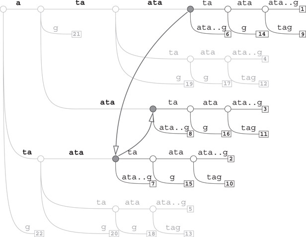
Figure 59.1The tree T_x for x = ataatataataatataatatag: subtrees rooted at solid gray nodes are isomorphic.

Subtree isomorphism can be checked by a classical linear-time algorithm by Aho et al. [31]. But on the suffix tree T_x this is done even more quickly once the f counts are available [32,33].

Lemma 59.2

Let T1 and T2 be two subtrees of T_x. T1 and T2 are isomorphic if and only if they have the same number of leaves and their roots are connected by a chain of suffix links.

If, during the bottom-up traversal of S_x, we collect in the same class strings such that their terminal arc leads to nodes with the same frequency counts f, then this would identify and produce the ≡_x-classes, that is, the smallest substring partition.

Example 59.3

For instance, starting from the right-equivalent class C = {ataata, taata, aata}, one can augment it with of all words which are left-equivalent to the elements of C. The result is one ≡_x-class composed by {ataa, ataat, ataata, taa, taat, taata, aa, aat, aata}. Their respective pos sets are {1,6, 9,14}, {1,6, 9,14}, {1,6, 9,14}, {2,7, 10,15}, {2,7, 10,15}, {2,7, 10,15}, {3,8, 11,16}, {3,8, 11,16}, {3,8, 11,16}. Their respective endpos sets are {4,9, 12,17}, {5,10, 13,18}, {6,11, 14,19}, {4,9, 12,17}, {5,10, 13,18}, {6,11, 14,19}, {4,9, 12,17}, {5,10, 13,18}, {6,11, 14,19}. Because of Lemma 59.1, given two words y and w in the class, either they share the start set, or they share the end set, or they share the start set by transitivity with a third word in the class, or they share the end set by transitivity with a third word in the class. It turns out that there are only seven ≡_x-classes in this example.

Note that the longest string in this ≡_x-class is unique (ataata) and that it contains all the others as substrings. The shortest string is unique as well (aa). As said, the number of occurrences for all the words in the same class is the same (4 in the example). Figure 59.2 illustrates the seven equivalence classes for the running example. The words in each class have been organized in a lattice, where edges correspond to extensions (or contractions) of a single symbol. In particular, horizontal edges correspond to right extensions and vertical edges to left extensions.

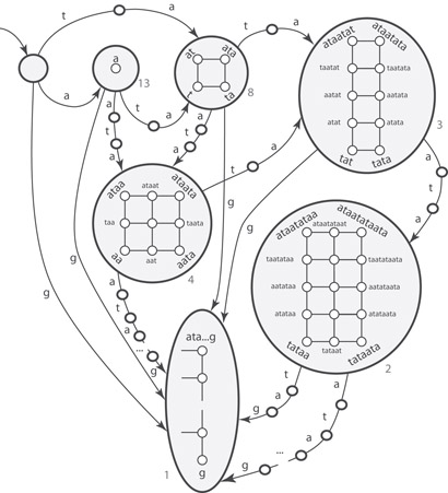
Figure 59.2A representation of the seven ≡_x-classes for x = ataatataataatataatatag. The words in each class can be organized in a lattice. Numbers refer to the number of occurrences.

While the longest word in an ≡_x-class is unique, there may be in general more than one shortest word. Consider, for example, the text x = akgk, with k > 0. Choosing k = 2 yields a class which has three words of length two as minimal elements, namely, aa, gg, and ag. (In fact, imp_x(aa) = imp_x(gg) = imp_x(ag) = aagg.) Taking instead k = 1, all three substrings of x = ag coalesce into a single class which has two shortest words.

Recall that by Lemma 59.1, each ≡_x-class C can be expressed as the union of one or more left-equivalent classes. Alternatively, C can be also expressed as the union of one or more right-equivalent classes. The example above shows that there are cases in which left- or right-equivalent classes cannot be merged without violating the uniqueness of the shortest word. Thus we may use the ≡_x-classes as the C_i’s in our partition only if we are interested in detecting overrepresented words. If underrepresented words are also wanted, then we must represent a same ≡_x-class once for each distinct shortest word in it.

It is not difficult to accommodate this in the subtree merge procedure. Let p(u) denote the parent of u in T_x. While traversing S_x bottom-up, merge two nodes u and v with the same f count if and only if both pairs (u, v) and (p(u), p(v)) are connected by a suffix link. This results in a substring partition slightly coarser than ≡_x. It will be denoted by $\tilde{\equiv_{x}}$ $\tilde{\equiv_{x}}$ .

Fact 59.2

Let {C1, C2, …, C_l} be the set of equivalence classes built on the equivalence relation $\tilde{\equiv_{x}}$ $\tilde{\equiv_{x}}$ on the substrings of text x. Then, for all 1 ≤ i ≤ l,

1. $max (C_{i})$ $max (C_{i})$ and $min (C_{i})$ $min (C_{i})$ are unique

2.All w ∈ C_i are on some $(min (C_{i}), max (C_{i}))$ $(min (C_{i}), max (C_{i}))$ -path

3.All w ∈ C_i have the same number of occurrences f_x(w).

We are now ready to address the computational complexity of our constructions. In Reference 21, linear-time algorithms are given to compute and store expected value E(Z_w) and variance Var(Z_w) for the number of occurrences under Bernoulli model of all prefixes of a given string. The crux of that construction rests on deriving an expression of the variance (see Expression 59.1) that can be cast within the classical linear time computation of the “failure function” or smallest periods for all prefixes of a string [31]. These computations are easily adapted to be carried out on the linked structure of graphs such as S_x or D_x, thereby yielding expectation and variance values at all nodes of T_x, D_x, or the compact variant of the latter. These constructions take time and space linear in the size of the graphs, hence linear in the length of x. Combined with the monotonicity results this yields immediately:

Theorem 59.2

Under the Bernoulli model [20], the sets $O_{z}^{T}$ $O_{z}^{T}$ and $U_{z}^{T}$ $U_{z}^{T}$ associated to the score

z (w) = \frac{f_{x} (w) - E (Z_{w})}{\sqrt{V a r (Z_{w})}}

$z (w) = \frac{f_{x} (w) - E (Z_{w})}{\sqrt{V a r (Z_{w})}}$

can be computed in linear time and space, provided that $p_{\max} < min {1 / \sqrt[m]{4 m}, \sqrt{2} - 1}$ $p_{\max} < min {1 / \sqrt[m]{4 m}, \sqrt{2} - 1}$ .

59.3Comparing Whole Genomes

As of writing this article (March 2015), Genbank contains “complete” genomes for more than 3900 virus, over 3200 bacterial, and about 180 eukaryote species. For many of these species, there are even several different genomes available. The abundance of complete genome sequences has given an enormous boost to comparative genomics. Association studies have become a powerful tool for the functional identification of genes and molecular genetics has in many cases revealed the biological basis of diversity. Comparing the genomes of related species gives new insights into the complex structure of organisms at the DNA level and protein level.

The first step when comparing genomes is to produce an alignment, that is, a collinear arrangement of sequence similarities. Alignment of nucleic or amino acid sequences has been one of the most important methods in sequence analysis, with much dedicated research and now many sophisticated algorithms available for aligning sequences with similar regions. These require defining a score for all possible alignments (typically, the sum of the similarity/identity values for each aligned symbol, minus a penalty for the introduction of gaps), along with a dynamic programming method to find optimal or near-optimal alignments according to this scoring scheme [34]. These dynamic programming methods run in time proportional to the product of the length of the sequences to be aligned. Hence they are not suitable for aligning entire genomes. In the last decade, a large number of genome alignment programs have been developed, most of which use an anchor-based method to compute an alignment (for an overview, see Reference 35). An anchor is an exact match of some minimum length occurring in all genomes to be aligned (see Figure 59.3). The anchor-based method can roughly be divided into the following three phases:

1.Computation of all potential anchors

2.Computation of an optimal collinear sequence of nonoverlapping potential anchors: these are the anchors that form the basis of the alignment (see Figure 59.4)

3.Closure of the gaps in between the anchors.

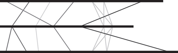
Figure 59.3Three genomes represented as horizontal lines. Potential anchors of an alignment are connected by vertical lines. Each anchor is a sequence occurring at least once in all three genomes.

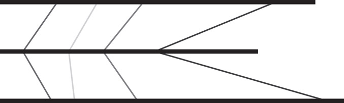
Figure 59.4A collinear chain of nonoverlapping anchors.

In the following, we will focus on phase 1 and describe two algorithms to compute potential anchors. The first algorithm allows one to align more than two genomes, while the second is limited to two genomes, but uses less space than the former. Both algorithms are based on suffix trees. For phase 2 of the anchor-based method, one uses methods from computational geometry. The interested reader is referred to the algorithms described in References 36–39. In phase 3, one can apply any standard multiple or pairwise alignment methods, such as T-Coffee [40] or MAFFT [41]. Alternatively, one can even use the same anchor-based method with relaxed parameters, like it is possible in the CoCoNUT software [42].

59.3.1Basic Definitions

We recall and extend the definition introduced in Section 59.2. A sequence, or a string, S of length n is written as S = S[0]S[1]…S[n−1] = S[0…n−1]. A prefix of S is a sequence S[0…i] for some i, 0 ≤ i ≤ n − 1. A suffix of S is a sequence S[i…n − 1] for some i, 0 ≤ i ≤ n − 1. Consider a set {G0,…, G_{k − 1}} of k ≥ 2 sequences (the genomes) over some alphabet Σ. Let n_q = |G_q| for 0 ≤ q ≤ k − 1. To simplify the handling of boundary cases, assume that G0[−1] = $₋₁ and G_{k − 1}[n_{k − 1}] = $_k−1 are unique symbols not occurring in Σ. A multiple exact match is a (k + 1)-tuple (l, p0, p1, …, p_k−1) such that l > 0, 0 ≤ p_q ≤ n_q−l, and G_q[p_q…p_q + l − 1] = G_q′[p_q′…p_q′ + l − 1] for all q, q′, 0 ≤ q, q′ ≤ k − 1. A multiple exact match is left maximal if for at least one pair (q, q′), 0 ≤ q, q′ ≤ k − 1, we have G_q[p_q − 1] ≠ G_q′[p_q′−1]. A multiple exact match is right maximal if for at least one pair (q, q′), 0 ≤ q, q′ ≤ k − 1, we have G_q [p_q + l] ≠ G_q′[p_q′ + l]. A multiple exact match is maximal if it is left maximal and right maximal. A maximal multiple exact match is also called multiMEM. Roughly speaking, a multiMEM is a sequence of length l that occurs in all sequences G0,…, G_{k − 1} (at positions p0,…, p_{k − 1}), and cannot simultaneously be extended to the left or to the right in every sequence. The ℓ-multiMEM-problem is to enumerate all multiMEMs of length at least ℓ for some given length threshold ℓ ≥ 1. For k = 2, we use the notion MEM and ℓ-MEM-problem. The notions of matches defined here can be generalized in several ways. One important generalization is to require that for all q, the matching substring G_q[p_q … p_q + l − 1] is allowed to occur at most r_q times in G_q for some user-defined parameter r_q. This allows to model, for example, maximal unique matches (by defining r_q = 1) or excludes repeats from being part of a multiMEM (by defining r_q as small constant). Methods to compute such rare multiple matches are described in Reference 74. Here we however restrict to solutions of the ℓ-multiMEM-problem.

Let $0,…,$_k−1 be pairwise different symbols not occurring in any G_q. These symbols are used to separate the sequences in the concatenation S = G0 $0G1 $1…G_k−2 $_k−2G_{k − 1}. $_k;−1 will be used as a sentinel attached to the end of G_{k − 1}. All these special symbols are collected in a set Seps = {$₋₁, $0,…, $_k−2, $_k−1}.

Let n = |S|. For any i, 0 ≤ i ≤ n, let S_i = S[i…n − 1] $_k−1 denote the ith nonempty suffix of S $_k−1. Hence S_n= $_k−1. For all q, 0 ≤ q ≤ k − 1 let t_q be the start position of G_q in S. For 0 ≤ i ≤ n − 1 such that S[i] ∉ Seps, let

•σ(i) = q iff position i occurs in the qth sequence in S and

•ρ(i) = i − t_q denote the relative position of i in G_q.

We consider trees whose edges are labeled by nonempty sequences. For each symbol a, every node α in these trees has at most one a-edge for some sequence v and some node β. Let $T$ $T$ be a tree and α be a node in $T$ $T$ . A node α is denoted by w if and only if w is the concatenation of the edge labels on the path from the root of $T$ $T$ to α. A sequence w occurs in $T$ $T$ if and only if $T$ $T$ contains a node $\bar{w v}$ $\bar{w v}$ , for some (possibly empty) sequence v. The suffix tree for S, denoted by ST(S), is the tree $T$ $T$ with the following properties: (i) each node is either the root, a leaf or a branching node, and (ii) a sequence w occurs in $T$ $T$ if and only if w is a substring of S $_k−1. For each branching node $\bar{a u}$ $\bar{a u}$ in ST(S), where a is a symbol and u is a string, u is also a branching node, and there is a suffix link from $\bar{a u}$ $\bar{a u}$ to $\bar{u}$ $\bar{u}$ .

There is a one-to-one correspondence between the leaves of ST(S) and the nonempty suffixes of S $_k−1: leaf $\bar{S_{i}}$ $\bar{S_{i}}$ corresponds to suffix S_i and vice versa.

For any node $\bar{u}$ $\bar{u}$ of ST(S) (including the leaves), let $P_{\bar{u}}$ $P_{\bar{u}}$ be the set of positions i such that u is a prefix of S_i. In other words, $P_{\bar{u}}$ $P_{\bar{u}}$ is the set of positions in S where sequence u starts. $P_{\bar{u}}$ $P_{\bar{u}}$ is divided into disjoint and possibly empty position sets:

•For any q, 0 ≤ q ≤ k − 1, define $P_{\bar{u}} (q) = {i \in P_{\bar{u}} ∣ σ (i) = q}$ $P_{\bar{u}} (q) = {i \in P_{\bar{u}} ∣ σ (i) = q}$ that is, $P_{\bar{u}}$ $P_{\bar{u}}$ (q) is the set of positions i in S where u starts and i is a position in genome G_q.

•For any a ∈ Σ ∪ Seps, define $P_{\bar{u}}$ $P_{\bar{u}}$ (a) = {i ∈ $P_{\bar{u}}$ $P_{\bar{u}}$ | S[i − 1] = a}, that is, $P_{\bar{u}}$ $P_{\bar{u}}$ (a) is the set of positions i in S where u starts and the symbol to the left of this position is a. We also state that the left context of i is a.

•For any q, 0 ≤ q ≤ k − 1 and any a ∈ Σ ∪ Seps, define $P_{\bar{u}}$ $P_{\bar{u}}$ (q, a) = $P_{\bar{u}}$ $P_{\bar{u}}$ (q) ∩ $P_{\bar{u}}$ $P_{\bar{u}}$ (a).

59.3.2Computation of multiMEMs

We now describe an algorithm to compute all multiMEMs, using the suffix tree for S. The algorithm is part of the the multiple genome alignment software MGA. It improves on the method which was described in Reference 72.

The algorithm computes position sets $P_{\bar{u}}$ $P_{\bar{u}}$ (q, a) by processing the edges of the suffix tree in a bottom-up traversal. That is, the edge leading to node $\bar{u}$ $\bar{u}$ is processed only after all edges in the subtree below $\bar{u}$ $\bar{u}$ have been processed.

If $\bar{u}$ $\bar{u}$ is a leaf corresponding to, say suffix S_i, then compute $P_{\bar{u}}$ $P_{\bar{u}}$ (q, a) = {i} where q = σ(i) and a = S[i − 1]. For all (q′, a′) ≠ (q, a) compute $P_{\bar{u}}$ $P_{\bar{u}}$ (q′, a′) = ∅. Now suppose that $\bar{u}$ $\bar{u}$ is a branching node with r outgoing edges. These are processed in any order. Consider an edge $\bar{u} ⟶ \bar{w}$ $\bar{u} ⟶ \bar{w}$ . Due to the bottom-up strategy, $P_{\bar{w}}$ $P_{\bar{w}}$ is already computed. However, only a subset of $P_{\bar{u}}$ $P_{\bar{u}}$ has been computed since only, say j < r, edges outgoing from $\bar{u}$ $\bar{u}$ have been processed. The corresponding subset of $P_{\bar{u}}$ $P_{\bar{u}}$ is denoted by $P_{\bar{u}}^{j}$ $P_{\bar{u}}^{j}$ . The edge $\bar{u} \to \bar{w}$ $\bar{u} \to \bar{w}$ is processed in the following way: at first, multiMEMs are output by combining the positions in $P_{\bar{u}}^{j}$ $P_{\bar{u}}^{j}$ and $P_{\bar{w}}$ $P_{\bar{w}}$ . In particular, all (k + 1)-tuples (l, p0, p1, …, p_{k − 1}) satisfying the following conditions are enumerated:

1.l = |u|

2.p_q ∈ $P_{\bar{u}}^{j}$ $P_{\bar{u}}^{j}$ (q)∪ $P_{\bar{w}}$ $P_{\bar{w}}$ (q) for any q, 0 ≤ q ≤ k − 1

3.p_q ∈ $P_{\bar{u}}^{j}$ $P_{\bar{u}}^{j}$ (q) for at least one q, 0 ≤ q ≤ k − 1

4.p_q ∈ $P_{\bar{w}}$ $P_{\bar{w}}$ (q) for at least one q, 0 ≤ q ≤ k − 1

5.p_q ∈ $P_{\bar{w}}$ $P_{\bar{w}}$ (q, a) and p_q′ ∈ $P_{\bar{w}}$ $P_{\bar{w}}$ (q′, b) for at least one pair (q, q′), 0 ≤ q, q′ ≤ k − 1 and different symbols a and b.

By definition of $P_{\bar{u}}$ $P_{\bar{u}}$ , u occurs at positions p0, p1, …, p_{k − 1} in S. Moreover, for all q, 0 ≤ q ≤ k − 1, we define ρ(p_q) as the relative position of u in G_q. Hence (l, ρ(p0), ρ(p1),…, ρ(p_{k − 1})) is a multiple exact match. Conditions 3 and 4 guarantee that not all positions are exclusively taken from $P_{\bar{u}}^{j}$ $P_{\bar{u}}^{j}$ (q) or from $P_{\bar{w}}$ $P_{\bar{w}}$ (q). In other words, at least two of the positions in {p0, p1,…, p_{k − 1}} are taken from different subtrees below $\bar{u}$ $\bar{u}$ . Suppose that p_q ∈ $P_{\bar{u}}^{j}$ $P_{\bar{u}}^{j}$ (q) and p_q′ ∈ $P_{\bar{w}}$ $P_{\bar{w}}$ (q′). Hence p_q comes from a subtree below $\bar{u}$ $\bar{u}$ that can be reached by one of the previous j edges processed so far. Let c be the first character of label of this edge. p_q′ comes from the subtree reached by $\bar{u} \to \bar{w}$ $\bar{u} \to \bar{w}$ and the first character of the label of this edge is different from c. As a consequence (l, ρ (p0), ρ(p1),…, ρ(p_{k − 1})) is right maximal. Condition 5 means that at least two of the positions in {p0, p1,…, p_{k − 1}} have a different left context. This implies that (l, ρ(p0), ρ(p1),…, ρ(p_{k − 1})) is left maximal.

As soon as for the current edge $\bar{u} \to \bar{w}$ $\bar{u} \to \bar{w}$ the multiMEMs are enumerated, the algorithm adds $P_{\bar{w}}$ $P_{\bar{w}}$ (q, a) to $P_{\bar{u}}^{j}$ $P_{\bar{u}}^{j}$ (q, a) to obtain position sets $P_{\bar{u}}^{j + 1}$ $P_{\bar{u}}^{j + 1}$ (q, a) for all q, 0 ≤ q ≤ k − 1 and all a ∈ Σ ∪ Seps. That is, the position sets are inherited from node $\bar{w}$ $\bar{w}$ to the parent node $\bar{u}$ $\bar{u}$ . Finally, $P_{\bar{u}}$ $P_{\bar{u}}$ (q, a) is obtained as soon as all edges outgoing from $\bar{u}$ $\bar{u}$ are processed.

The algorithm performs two operations on position sets, namely enumeration of multiple exact matches by combining position sets and accumulation of position sets. A position set $P_{\bar{u}}$ $P_{\bar{u}}$ (q, a) is the union of position sets from the subtrees below $\bar{u}$ $\bar{u}$ . Recall that we consider processing an edge $\bar{u} \to \bar{w}$ $\bar{u} \to \bar{w}$ . If the edges to the children of $\bar{w}$ $\bar{w}$ have been processed, the position sets of the children are obsolete. Hence it is not required to copy position sets. At any time of the algorithm, each position is included in exactly one position set. Thus the position sets require O(n) space. For each branching node one maintains a table of k(|Σ| + 1) references to possibly empty position sets. In particular, to achieve independence of the number of separator symbols, we store all positions from $P_{\bar{u}}$ $P_{\bar{u}}$ (q, a), a ∈ Seps, in a single set. Hence, the space requirement for the position sets is O(|Σ|kn). The union operation for the position sets can be implemented in constant time using linked lists. For each node, there are O(|Σ|k) union operations. Since there are O(n) edges in the suffix tree, the union operations thus require O(|Σ|kn) time.

Each combination of position sets requires to enumerate the following cartesian product:

	(59.2)

The enumeration is done in three steps, as follows. In a first step one enumerates all possible k-tuples (P0, P1,…, P_{k − 1}) of nonempty sets where each P_q is either $P_{\bar{u}}^{j}$ $P_{\bar{u}}^{j}$ (q) or $P_{\bar{w}}$ $P_{\bar{w}}$ (q). Such a k-tuple is called father/child choice, since it specifies to either choose a position from the father $\bar{u}$ $\bar{u}$ (a father choice) or from the child $\bar{w}$ $\bar{w}$ (a child choice). One rejects the two k-tuples specifying only father choices or only child choices and processes the remaining father/child choices further. In the second step, for a fixed father/child choice (P0, P1, … , P_{k − 1}) one enumerates all possible k-tuples (a0, … , a_{k − 1}) (called symbol choices) such that P_q(a_q) ≠ ∅. At most |Σ| symbol choices consisting of k identical symbols (this can be decided in constant time) are rejected. The remaining symbol choices are processed further. In the third step, for a fixed symbol choice (a0, … , a_{k − 1}) we enumerate all possible k-tuples (p0, … , p_{k − 1}) such that p_q ∈ P_q(a_q) for 0 ≤ q ≤ k − 1. By construction, each of these k-tuples represents a multiMEM of length l. The cartesian product (59.2) thus can be enumerated in O(k) space and in time proportional to its size.

The suffix tree construction and the bottom-up traversal (without handling of position sets) require O(n) time. Thus the algorithm described here runs in O(|Σ|kn) space and O(|Σ|kn + z) time where z is the number of multiMEMs. It is still unclear if there is an algorithm which avoids the factors |Σ| or k in the space or time requirement.

59.3.3Space Efficient Computation of MEMs for Two Genomes

The previous algorithm, when applied to two genomes, requires to construct the suffix tree of the concatenation S = G0 $0G1. The algorithm described next computes all MEMs of length at least ℓ by constructing the suffix tree of G0 and matches G1 against it. Thus, for genomes of similar sizes, the space requirement is roughly halved.

The matching process delivers substrings of G1 represented by locations in the suffix tree, where a location is defined as follows: Suppose a string u occurs in ST(G0). If there is a branching node $\bar{u}$ $\bar{u}$ , then $\bar{u}$ $\bar{u}$ is the location of u. If $\bar{v}$ $\bar{v}$ is the branching node of maximal depth, such that u = vw for some nonempty string w, then ( $\bar{v}$ $\bar{v}$ , w) is the location of u. The location of u is denoted by loc(u).

ST(G0) represents all suffixes T_i = G0[i…n0−1] $0 of G0 $0. The algorithm processes G1 suffix by suffix from longest to shortest. In the jth step, the algorithm processes suffix R_j = G1[j…n1−1] $2 and computes the locations of two prefixes pjmin and pjmax of R_j defined as follows:

•pjmax is the longest prefix of R_j that occurs in ST(G0).

•pjmin is the prefix of pjmax of length min{ℓ,|pjmax|}.

If |pjmin| < ℓ, then pjmin = pjmax and the longest prefix of R_j matching any substring of G1 is not long enough. So in this case R_j is skipped. If |pjmin| = ℓ, then at least one suffix represented in the subtree below loc(pjmin) matches the first ℓ characters of R_j. To extract the MEMs, this subtree is traversed in a depth first order. The depth first traversal maintains for each visited branching node u the length of the longest common prefix of u and R_j. Each time a leaf ${\bar{T}}_{i}$ ${\bar{T}}_{i}$ is visited, one first checks if G0[i − 1] ≠ G1[j − 1]. If this is the case, then (⊥, ρ(i), ρ(j)) is a left maximal exact match and one determines the length l of the longest common prefix of T_i and R_j. By construction, l ≥ ℓ and G0[i + l] ≠ G1[j + l]. Hence (l, ρ(i), ρ(j)) is an MEM. Now consider the different steps of the algorithm in more detail.

Computation of loc(pjmin): For j = 0, one computes loc(pjmin) by greedily matching G1[0…ℓ−1] against ST(G0). For all j, 1 ≤ j ≤ n1−1, one follows the suffix link of loc $(p_{min}^{j - 1})$ $(p_{min}^{j - 1})$ , if this is a branching node, or of $\bar{v}$ $\bar{v}$ if loc $(p_{min}^{j - 1}) = (\bar{v}, w)$ $(p_{min}^{j - 1}) = (\bar{v}, w)$ . This shortcut via the suffix link leads to a branching node on the path from the root to loc(pjmin), from which one matches the next characters in G1. The method is similar to the matching statistics computation of Reference 43, and one can show that its overall running time for the computation of all loc(pjmin), 0 ≤ j ≤ n1−1, is O(n1).

Computation of loc(pjmax): Starting from loc(pjmin) one computes loc(pjmax) by greedily matching G1[|pjmin|…n_j−1] against ST(G0). To facilitate the computation of longest common prefixes, one keeps track of the list of branching nodes on the path from loc(pjmin) to loc(pjmax). This list is called the match path. Since $| p_{max}^{j - 1} | \geq 1$ $| p_{max}^{j - 1} | \geq 1$ implies $| p_{max}^{j} | \geq | p_{max}^{j - 1} | - 1$ $| p_{max}^{j} | \geq | p_{max}^{j - 1} | - 1$ , we do not always have to match the edges of the suffix tree completely against the corresponding substring of G1. Instead, to reach loc(pjmax), one rescans most of the edges by only looking at the first character of the edge label to determine the appropriate edge to follow. Thus the total time for this step in O(n1 + α) where α is the total length of all match paths. α is upper bounded by the total size β of the subtrees below loc(pjmin), 0 ≤ j ≤ n1−1. β is upper bounded by the number r of right maximal exact matches between G0 and G1. Hence the running time for this step of the algorithm is O(n1 + r).

The depth first traversal: This maintains an lcp-stack which stores for each visited branching node, say $\bar{u}$ $\bar{u}$ , a pair of values (onmatchpath, lcpvalue), where the Boolean value onmatchpath is true, if and only $\bar{u}$ $\bar{u}$ is on the match path, and lcpvalue stores the length of the longest common prefix of u and R_j. Given the match path, the lcp-stack can be maintained in constant time for each branching node visited. For each leaf ${\bar{T}}_{i}$ ${\bar{T}}_{i}$ visited during the depth first traversal, the lcp-stack allows to determine in constant time the length of the longest common prefix of T_i and R_j. As a consequence, the depth first traversal requires time proportional to the size of the subtree. Thus the total time for all depth first traversals of the subtrees below loc(pjmin), 0 ≤ j ≤ n1−1, is O(r).

Altogether, the algorithm described here runs in O(n0 + n1 + r) time and O(n0) space. It is implemented as part of the widely used MUMmer genome alignment software [44] which is available at http://mummer.sourceforge.net/.

59.4The FM-index

In the last decade, next-generation sequencing (NGS) machines have become the main tool for genomic analysis. The widespread diffusion of NGS machines and their continuous increase in efficiency have posed new challenges to the bioinformatics community. Usually, the first step in the analysis of NGS data is the alignment of millions of short (a few hundred bases) fragments to a reference genome. Such alignment is indeed an approximate matching problem since fragments can differ from the reference because of sequencing errors or individual differences. Because of the importance of the problem it is not surprising that many different alignment tools have been proposed in the literature [45,46]. Some of the most popular alignment tools, such as Bowtie2 [47], BWA-MEM [48], GEM [49], and Soap2 [50], solve the “inexact” alignment problem by first finding exact matches between substrings of the fragment and the reference genome. The FM-index has also been used in some genome assembly tools (e.g., SGA [51]).

Because of the size of the data involved, to find such exact matches these tools do not use the suffix array or suffix tree data structures introduced in Chapters 30 and 31. Instead, they use some variant of the more recent FM-index data structure described in this section. As we will see the FM-index is strictly related to the suffix array but it is much more compact and searches for exact matchings using a completely different, and somewhat surprising, strategy in which the problem of searching substrings is reduced to the easier problem of counting single characters.

Figure 59.5 shows the suffix array for the string agaatatagtag $, where, as usual, we have introduced a unique sentinel character $ which is lexicographically smaller than all other symbols. On the right of the suffix array we show the matrix of characters obtained by transforming each suffix into a cyclic rotation of the input string. In the matrix we have highlighted the first (F) and last (L) columns. It is immediate to see that any column of this matrix, hence also F and L, is a permutation of the input string. Clearly column F contains the string characters alphabetically sorted, while the last column L has no apparent properties. The following result, due to Mike Burrows and David Wheeler, shows that indeed these two columns are related by the following nontrivial property.

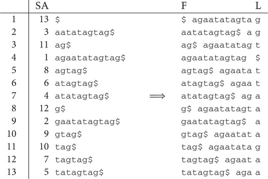
Figure 59.5Suffix array and Burrows–Wheeler transform for the string s = agaatatagtag$.

Theorem 59.3

For any character α [52], the ith occurrence of α in L corresponds to the ith occurrence of α in F.

For example, in Figure 59.5 the second a in L and F are respectively L[8] and F[3]; these two characters coincide in the sense that they are both the last a of the input string agaatatagtag$. In view of the above property, it is natural to define the Last-to-First column mapping LF, such that LF(i) is the index in the first column F of the character corresponding to L[i]. For example since L[8] corresponds to F[3] we have LF(8) = 3. As another example LF(2) = 9 since L[2], the second occurrence of g in L, corresponds to F[9], the second occurrence of g in F; indeed they are both the first g in agaatatagtag$.

Let C denote the array indexed by characters in Σ such that C[α] is the number of occurrences of text characters alphabetically smaller than α, and let Rank_α(L, k) denote the number of occurrences of the character α in the prefix L[1, k]. By Theorem 59.3, if L[i] = α then the character in column F corresponding to L[i] is the Rank_α(L, i)-th occurrence of α in F. Since the characters in F are alphabetically sorted, this occurrence is in position C[α] + Rank_α(L, i). Summing up, we have that the LF map can be computed as

$L F (i) = C [L [i]] + {Rank}_{L [i]} (L, i)$ $L F (i) = C [L [i]] + {Rank}_{L [i]} (L, i)$	(59.3)

Given the last column L and the LF map, it is possible to retrieve the original string s because of the following observation: since each row j is a cyclic rotation of s, character L[j] immediately precedes F[j] in s, and L[LF(j)] immediately precedes L(j) = F[LF(j)]. Given L we can therefore retrieve s as follows: (i) compute F sorting the characters in L; (ii) by construction, the special character $ will be in F[1], hence the last character of s is s[n] = L[1]; (iii) by the above observation we have s[n − 1] = L[LF(1)], s[n − 2] = L[LF(LF(1))], and by induction s[n − i] = L[LFi(1)], where LFi(·) = LF(LF^{i − 1}(·)).

The function mapping the string s to the last column L is therefore an invertible transformation, now called the Burrows–Wheeler Transform. In Reference 52, Burrows and Wheeler not only proved the reversibility of the transformation but also noted that column L is often easy to compress and thus originated the family of the so - called Burrows - - Wheeler compressors (for further reading, see Reference [53] and references therein).

In the context of computational biology, rather than in its compressibility, we are interested in another remarkable property of the Burrows–Wheeler Transform. As we now show, because of its relationship with the suffix array, column L can be used as a full - text index for the original string s. This property was first established in Reference 54 and it is based on the following result.

Theorem 59.4

Let SA(s) denote the suffix array of the string s [54]. Assume that [begin,end] denotes the range of rows of SA(s) prefixed by a given pattern Q, where Q is a substring of s. Then, for any character α, the range of rows [begin′,end′] prefixed by αQ is given by

	(59.4)

If begin′>end′ then no row in SA(s) is prefixed by αQ, hence the pattern αQ does not appear inside s.

The above theorem follows from the observation that [begin′,end′] are precisely the positions in column F corresponding, via the LF-map, to the occurrences of α in L[begin,end]. This means that begin′ = LF(i) (resp. end′ = LF(j)), where i (resp. j) is the index of the first (resp. last) position in L[begin,end] containing the character α. Note that Equation 59.4 computes begin′ and end′ without actually computing the two indices i and j. From Theorem 59.4, we immediately get the procedure get_rows in Figure 59.6 for determining the rows of SA(s) prefixed by an arbitrary pattern P.

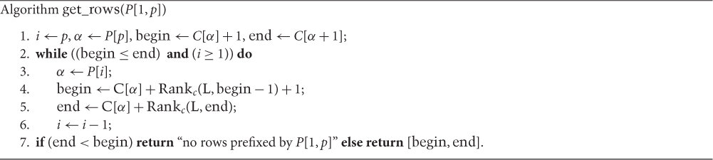
Figure 59.6Algorithm getrows for finding the set of suffix array rows prefixed by P[1, p]. This procedure is known in the literature as “backward search” since the characters of P are considered right to left.

Note that Theorem 59.4 and Algorithm get_rows determine a range of rows in SA(s) without using SA(s). The algorithm relies only on the array C, which has size |Σ|, and the computation of the function Rank_α(L,·). Indeed, the problem of searching substrings in s is reduced to the problem of counting single characters in L. The FM-index is loosely defined as a data structure taking O(|s|) bits of space and supporting the Rank operation in constant time [55]; if the alphabet is not constant, both space and time can have an additional O(polylog(|Σ|)) factor.

Using algorithm get_rows an FM-index can report the number of occurrences of a pattern P in s in O(|P|) time using O(|s|) bits of space. The same problem can be solved by a suffix array in O(|P| log n) time, or in O(|P| + log n) time using also the LCP array (see Chapters 30 and 31). Given the simplicity of the binary search procedure, the suffix array is likely to be faster in practice. However, the suffix array uses O(|s| log |s|) bits of space that, both in theory and in practice, is significantly larger than the space usage of FM-index [56]. Indeed, a remarkable feature of the FM-index is that it can take advantage of the compressibility of the input string. Exploiting properties of the Burrows - Wheeler Transform, the FM-index can be stored in space asymptotically bounded by the kth‐order entropy of the sequence s and still support the Rank operation in constant time [57–59]. The kth‐order entropy is a natural lower bound for the compressibility of a sequence and it was somewhat surprising that in such a “minimal” space we can not only represent s but also search it.

In some applications, we are interested not only in counting the occurrences but also in finding their positions within s. For this task, the speed of the suffix array is hard to beat: once the range of rows [begin,end] is determined the positions are simply the values stored in SA[begin…end]. To efficiently solve the same problem on an FM-index it is necessary to enrich it with additional information. The common approach is to store along with the FM-index a sampling of the suffix array. For example, we can store the values SA[i] which are multiples of a given value d. Then, using a hash table or a bit array (possibly compressed), we mark the rows containing the stored values.

In the example of Figure 59.5, if we take d = 4, we mark the rows {5,7,8} since they contains the SA values {8,4,12}. To determine the position of the occurrences of the pattern tag we first use algorithm get_rows to find the SA rows prefixed by tag, which are the rows 11 and 12 of the suffix array. Then, we proceed determining the position in s of these two rows (or more precisely of the two suffixes prefixing these two rows). If we had the complete suffix array the desired values SA[11] = 10 and SA[12] = 7 would be immediately available, but we only have the SA values for the rows {5,7,8}. To determine for example SA[11], we apply the LF-map (59.3) and compute the value 10 = LF(11) which is the entry in F corresponding to the character L[11] = g. By construction, we have that row 10 contains the suffix which is one character longer than the suffix in row 11, hence SA[10] = SA[11]−1. Since row 10 is not marked, we still do not know the value SA[10]. We thus compute LF(10) = 5, which is the index of the row containing the suffix one character longer than the one in row 10. Reasoning as above we have

SA [5] = SA [10] - 1 = SA [11] - 2.

$SA [5] = SA [10] - 1 = SA [11] - 2.$

Now we find that row 5 is marked hence the value SA[5] = 8 is available, from which we correctly derive SA[11] = 10. The above procedure for retrieving the position of a single occurrence is formalized in Figure 59.7. The idea is to use the LF-map to move backward in the text until we reach a marked position for which the SA value is known. By construction we reach a marked position in at most d − 1 steps, so the cost of locating a single occurrence is bounded by d times the cost of a Rank operation. Since the cost of storing the SA values is O(n log n)/d bits, the parameter d offers a simple trade-off between memory usage and speed.

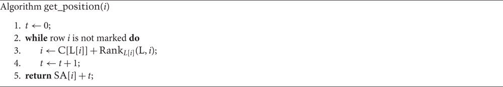
Figure 59.7Algorithm get_position for the computation of SA[i] on an FM-index enriched with a sample of the suffix array. Note that the value computed at line 3 is LF(i) (cf. Equation 59.3).

Although the above simple strategy works well in most cases, improvements or other approaches to the problem of locating the occurrences using an FM-index have been proposed in the literature. The reader should refer to References 60–62 and references therein for further information.

59.4.1Fast Rank and Select Operations Using Wavelet Trees

Wavelet trees have been introduced in Reference 71 at roughly the same time as compressed indices and have quickly gained popularity as a very versatile data structure. They can be described as a data structure offering some degree of compression and supporting fast Rank/Select operations (see below), but over the years they have been used to provide elegant and efficient solutions for a myriad of problems in different algorithmic areas [63].

Consider again the string s of Figure 59.5 and let s′ = ggt$ttaaaagaa denote its Burrows - - Wheeler transform, that is, column L of Figure 59.5. Figure 59.8 shows a wavelet tree for the string s′. The tree is a complete binary tree and each leaf corresponds to an alphabet character. To build the wavelet tree, we initially label the root with the string s′. Then at each internal node each character goes left or right depending on whether the leaf labeled with that character is on the left or the right subtree. So for example at the root $ and a both go left, while at the root’s left child $ goes left and a goes right. Finally, we replace each string in the internal nodes with a binary string obtained replacing with 0 each character that goes left, and with 1 each character that goes right. The wavelet tree consists of the set of binary strings associated to the internal nodes; in our example the wavelet tree for s′ = ggt$ttaaaagaa is represented by the binary strings w_root = 1110110000100, w_left = 0111111, w_right = 011110 (we are assuming the shape of the tree and the correspondence from leaves to characters are established in advance so there is no need to encode them).

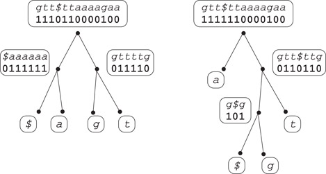
Figure 59.8Two wavelet trees of different shapes for the string s′ = ggt$ttaaaagaa. The tree on the left is balanced and has all leaves at depth two. The tree on the right has the leaf associated to a at depth one: as a result it uses three less bits in the internal nodes.

Suppose now that we are given the wavelet tree and we want to retrieve the character s′[6]. Since w_root[6] = 1 we know that it is a character on the right subtree, so either g or t. To find out which, we count how many 1’s there are in w_root up to position 6. Using the notation of the previous section this number is Rank1(w_root, 6) = 5. Hence, s′[6] corresponds to the fifth bit of w_right. Since w_right[5] = 1 and w_right’s right child is the leaf labeled t we have s′[6] = t. From the above decoding procedure, we can draw the following observations:

1.Each character in the input text is essentially encoded with one bit for each internal node in the path from the root to the corresponding leaf. Using a balanced tree each character requires at most ⌈ log |Σ|⌉ bits so the total space usage will be similar to the space used for s′ uncompressed. However, using a tree of different shape we can represent s′ with less bits (see the tree on the right in Figure 59.8). For any input string, we can minimize the overall length of the internal node’s binary strings using the shape of an optimal Huffman tree. Note that the resulting data structure would offer essentially the same compression as a Huffman code but it will also provide random access to the single characters, something which is not possible with Huffman codes. For further discussions on the compressibility of wavelet trees, see Reference 64 and references therein.

2.Assuming that the computation of Rank1 on a binary string takes O(r) time, decoding a single input character with the above procedure on a balanced wavelet tree takes O(r log |Σ|) time (notice that Rank0(w, k) = k − Rank1(w, k)). If the wavelet tree is skewed some characters could be more expensive to decode than others. For example, if we use a Huffman - shaped tree decoding will be faster for frequent characters and slower for those rarely occurring, a trade - off that could be appropriate in some situations. More in general, if we know the distribution of the accesses we can sacrifice space and choose the shape of the wavelet tree in order to minimize the average access time.

The above observations show that wavelet trees are interesting per se. However, their use for FM - indices is justified by another remarkable property. Recall that to efficiently search for patterns in s an FM-index need to support efficient Rank operations on s′. Consider again the example of Figures 59.5 and 59.8 and suppose we need to compute Rank_a(s′,9), that is, count how many a’s are there in the first nine positions of s′. In the string w_root a is represented by 0, so by computing Rank0(w_root,9) = 4 we find that in the first nine positions of s′ there are four occurrences of $’s and a’s. To compute Rank_a(s′, 9), we need to count how many a’s are there among these four occurrences. This can be done looking at w_left: since there a is represented with a 1, we compute ${Rank}_{1} (w_{l e f t}, 4) = 3$ ${Rank}_{1} (w_{l e f t}, 4) = 3$ and this is precisely the value Rank_a(s′, 9) that we were looking for. Summing up, Rank queries on s′ for any character α can be resolved by Rank0/Rank1 queries on the nodes on the path from the root to the leaf associated to α. Note that, again, the wavelet tree shape influences the cost of the Rank queries on s′.

Putting all together, we have that combining FM-indices and wavelet trees the “difficult” problem of locating patterns in a reference text is reduced to the easier problem of computing Rank queries on binary strings (see Figure 59.9). Note that with an appropriate compressed representation of the binary strings and the use of compression boosting [65], the resulting data structure takes space close to the information theoretic lower bound given by the kth‐order entropy of the indexed sequence [66].

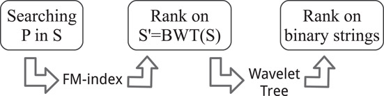
Figure 59.9The problem of searching patterns in a string is reduced to the problem of counting 1’s in binary strings thanks to the combined use of the FM-index and the wavelet tree data structure.

Computing Rank queries on binary strings is by no means trivial if we want to compress the binary strings involved. However, if the space usage is not a major issue, there are simple data structures for this task that even first-year students can easily implement. For example, suppose we want to support Rank1 operations on a binary string w (recall Rank0 values can be obtained by difference). We split the content of w into blocks of 256 bits and we store each block into four 64-bit words. We interleave these blocks with additional 64-bit words storing the number of 1’s in all the preceding blocks. These interleaved values are represented in gray in Figure 59.10.

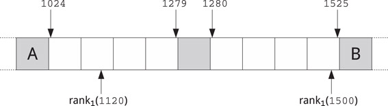
Figure 59.10Simple scheme supporting Rank queries on a binary string described in Reference 67. Each cell represents a 64-bit word. Four consecutive white cells contain a 256-bit block from input string, each gray cell contains the number of 1’s in the preceding blocks. The figure shows the 5th and 6th blocks of the input string containing bit ranges [1024, 1279] and [1280, 1525], respectively. Cell A stores the number of 1’s in [0, 1023], cell B stores the number of 1’s in [0, 1525].

To compute Rank1(w, k), we first locate the block containing w[k]. If w[k] is in the first half of the block we sum the value in the immediately preceding gray cell with the number of 1’s from said cell up to position k. Otherwise, if w[k] is in the second half of a block, we subtract from the value stored in the immediately following gray cell the number of 1’s from position k + 1 up to that cell. For example, in Figure 59.10 to compute Rank1(1120) we sum the value in A to the number of 1’s in [1024, 1120], while to compute Rank1(1500) we subtract from the value in B the number of 1’s in [1501, 1525].

Summing up, using the above data structure the computation of Rank1(w, k) only requires the access to up to three consecutive 64-bit words and counting the 1’s in up to two of them. Since the latter operation is natively supported by modern Intel and AMD processors (under the name POPCNT), the whole procedure is extremely fast and simple to implement. This data structure uses one additional 64-bit word for each 256-bit block, so the total space usage in bits is 1.25|w|. If we use this simple scheme for the binary strings of a wavelet tree, a representation of the Burrow–Wheeler Transform for the human genome (≈3 billion bases) would take less than 1 GB. Adding a sampling of the suffix array, say with d = 20, we get an FM-index of roughly 1.5 GB: this is almost 10 times smaller than the 12 GB used by the suffix array alone.

Together with the Rank operation many data structures support also its inverse, called Select. By definition Select_α(s′, k) is the position in s′ of the kth occurrence of character α, or some invalid value if α appears less than k times. As for the Rank operation, given a wavelet tree for s′, we can compute Select_α(s′, k) performing Select0/Select1 operations on the binary strings associated to the nodes in the path from the leaf associated to α up to the tree root (i.e., for Select we traverse the tree upward rather than downward). Computing Select on s′ = Bwt(s) allows us to compute the inverse of the LF-map in an FM-index which is useful, for example, for extracting substrings of the indexed text s [59].

For a discussion of sophisticated schemes for Rank/Select queries offering a variety of time/space trade-offs the reader should refer to Reference 59 for the theoretical results, and to References 67–69 for implementations and extensive experiments. The SDSL library [70] offers efficient and ready to use implementations of succinct (compressed) data structures including FM-indices, Suffix trees, and Wavelet trees.

References

1.R. Staden. Methods for discovering novel motifs in nucleic acid sequences. Comput. Appl. Biosci., 5(5), 1989, 293–298.

2.C. Burge, A. Campbell, and S. Karlin. Over- and under-representation of short oligonucleotides in DNA sequences. Proc. Natl. Acad. Sci. U.S.A., 89, 1992, 1358–1362.

3.T. Castrignano, A. Colosimo, S. Morante, V. Parisi, and G. C. Rossi. A study of oligonucleotide occurrence distributions in DNA coding segments. J. Theor. Biol., 184(4), 1997, 451–469.

4.J. W. Fickett, D. C. Torney, and D. R. Wolf. Base compositional structure of genomes. Genomics, 13, 1992, 1056–1064.

5.S. Karlin, C. Burge, and A. M. Campbell. Statistical analyses of counts and distributions of restriction sites in DNA sequences. Nucleic Acids Res., 20, 1992, 1363–1370.

6.R. Nussinov. The universal dinucleotide asymmetry rules in DNA and the amino acid codon choice. J. Mol. Evol., 17, 1981, 237–244.

7.P. A. Pevzner, M. Y. Borodovsky, and A. A. Mironov. Linguistics of nucleotides sequences II: Stationary words in genetic texts and the zonal structure of DNA. J. Biomol. Struct. Dyn., 6, 1989, 1027–1038.

8.G. J. Phillips, J. Arnold, and R. Ivarie. The effect of codon usage on the oligonucleotide composition of the E. coli genome and identification of over- and underrepresented sequences by Markov chain analysis. Nucleic Acids Res., 15, 1987, 2627–2638.

9.S. Volinia, R. Gambari, F. Bernardi, and I. Barrai. Co-localization of rare oligonucleotides and regulatory elements in mammalian upstream gene regions. J. Mol. Biol., 1(5), 1989, 33–40.

10.S. Volinia, R. Gambari, F. Bernardi, and I. Barrai. The frequency of oligonucleotides in mammalian genic regions. Comput. Appl. Biosci., 5(1), 1989, 33–40.

11.Predicting gene regulatory elements in silico on a genomic scale. Genome Res., 8(11), 1998, 1202–1215.

12.M. S. Gelfand, E. V. Koonin, and A. A. Mironov. Prediction of transcription regulatory sites in archaea by a comparative genomic approach. Nucleic Acids Res., 28(3), 2000, 695–705.

13.J. van Helden, B. André, and J. Collado-Vides. Extracting regulatory sites from the upstream region of the yeast genes by computational analysis of oligonucleotides. J. Mol. Biol., 281, 1998, 827–842.

14.J. van Helden, A. F. Rios, and J. Collado-Vides. Discovering regulatory elements in non-coding sequences by analysis of spaced dyads. Nucleic Acids Res., 28(8), 2000, 1808–1818.

15.M. S. Gelfand and E. V. Koonin. Avoidance of palindromic words in bacterial and archaeal genomes: A close connection with restriction enzymes. Nucleic Acids Res., 25, 1997, 2430–2439.

16.G. Reinert, S. Schbath, and M. S. Waterman. Probabilistic and statistical properties of words: An overview. J. Comput. Biol., 7, 2000, 1–46.

17.M. Lothaire. Ed. Combinatorics on Words. second ed. Cambridge University Press, London, 1997.

18.M. Lothaire Ed. Algebraic Combinatorics on Words. Cambridge University Press, London, 2002.

19.M. Tompa. An exact method for finding short motifs in sequences, with application to the ribosome binding site problem. In Proceedings of the 7th International Conference on Intelligent Systems for Molecular Biology, 1999, AAAI Press, Menlo Park, CA, pp. 262–271.

20.A. Apostolico, M. E. Bock, and S. Lonardi. Monotony of surprise and large-scale quest for unusual words. In Proceedings of Research in Computational Molecular Biology (RECOMB), Washington, DC, 2002. G. Myers, S. Hannenhalli, S. Istrail, P. Pevzner, and M. Waterman, Eds., Also in J. Comput. Biol., 10:3–4, (July 2003), 283–311.

21.A. Apostolico, M. E. Bock, S. Lonardi, and X. Xu. Efficient detection of unusual words. J. Comput. Biol., 7(1/2), Jan 2000, 71–94.

22.A. Apostolico, M. E. Bock, and X. Xu. Annotated statistical indices for sequence analysis. In Sequences, Positano, Italy, 1998, B. Carpentieri, A. De Santis, U. Vaccaro and J. Storer, Eds., IEEE Computer Society Press, pp. 215–229.

23.J. Gentleman. The distribution of the frequency of subsequences in alphabetic sequences, as exemplified by deoxyribonucleic acid. Appl. Statist., 43, 1994, 404–414.

24.J. Kleffe and M. Borodovsky. First and second moment of counts of words in random texts generated by Markov chains. Comput. Appl. Biosci., 8, 1992, 433–441.

25.P. A. Pevzner, M. Y. Borodovsky, and A. A. Mironov. Linguistics of nucleotides sequences I: The significance of deviations from mean statistical characteristics and prediction of the frequencies of occurrence of words. J. Biomol. Struct. Dy., 6, 1989, 1013–1026.

26.M. Régnier and W. Szpankowski. On pattern frequency occurrences in a Markovian sequence. Algorithmica, 22, 1998, 631–649.

27.E. Stückle, C. Emmrich, U. Grob, and P. Nielsen. Statistical analysis of nucleotide sequences. Nucleic Acids Res., 18(22), 1990, 6641–6647.

28.M. Y. Leung, G. M. Marsh, and T. P. Speed. Over and underrepresentation of short DNA words in herpesvirus genomes. J. Comput. Biol., 3, 1996, 345–360.

29.A. Blumer, J. Blumer, A. Ehrenfeucht, D. Haussler, and R. McConnel. Complete inverted files for efficient text retrieval and analysis. J. Assoc. Comput. Mach., 34(3), 1987, 578–595.

30.B. Clift, D. Haussler, R. McConnell, T. D. Schneider, and G. D. Stormo. Sequences landscapes. Nucleic Acids Res., 14, 1986, 141–158.

31.A. V. Aho, J. E. Hopcroft, and J. D. Ullman. The Design and Analysis of Computer Algorithms. Addison-Wesley, Reading, MA, 1974.

32.A. Apostolico and S. Lonardi. A speed-up for the commute between subword trees and DAWGs. Inf. Process. Lett., 83(3), 2002, 159–161.

33.D. Gusfield. Algorithms on Strings, Trees, and Sequences: Computer Science and Computational Biology. Cambridge University Press, 1997.

34.S. B. Needleman and C. D. Wunsch. A general method applicable to the search for similarities in the amino acid sequence of two proteins. J. Mol. Biol., 48, 1970, 443–453.

35.P. Chain, S. Kurtz, E. Ohlebusch, and T. Slezak. An applications-focused review of comparative genomics tools: Capabilities, limitations and future challenges. Brief. Bioinform, 4(2), 2003, 105–123.

36.M. I. Abouelhoda and E. Ohlebusch. A local chaining algorithm and its applications in comparative genomics. In Proceedings of the Third Workshop on Algorithms in Bioinformatics, WABI 2003, vol. 2812 of Lecture Notes in Computer Science, Springer Verlag, Budapest, Hungary, pp. 1–16.

37.M. I. Abouelhoda and E. Ohlebusch. Multiple genome alignment: Chaining algorithms revisited. In Proceeding of the 14th Annual Symposium on Combinatorial Pattern Matching CPM, 2003, Springer Verlag, Morelia, Mexico, pp. 1–16.

38.E. W. Myers and W. Miller. Chaining multiple-alignment fragments in sub-quadratic time. In Proceedings of the 6th ACM–SIAM Annual Symposium on Discrete Algorithms, 1995, San Francisco, CA, pp. 38–47.

39.Z. Zhang, B. Raghavachari, R. Hardison, and W. Miller. Chaining multiple alignment blocks. J. Comput. Biol., 1(3), 1994, 217–226.

40.C. Notredame, D. G. Higgins, and J. Heringa. T-Coffee: A novel method for fast and accurate multiple sequence alignment. J. Mol. Biol., 302(1), 2000, 205–217.

41.K. Katoh and D. M. Standley. MAFFT multiple sequence alignment software version 7: Improvements in performance and usability. Mol. Biol. Evol., 30(4), 2013, 772–780.

42.M. I. Abouelhoda, S. Kurtz, and E. Ohlebusch. CoCoNUT: An efficient system for the comparison and analysis of genomes. BMC Bioinformatics, 9, 2008, 476.

43.W. I. Chang and E. L. Lawler. Sublinear approximate string matching and biological applications. Algorithmica, 12(4/5), 1994, 327–344.

44.S. Kurtz, A. Phillippy, A. Delcher, M. Smoot, M. Shumway, C. Antonescu, and S. Salzberg. Versatile and open software for comparing large genomes. Genome Biol., 5(R12), 2004. https://genomebiology.biomedcentral.com/articles/10.1186/gb-2004-5-2-r12

45.N. Fonseca, J. Rung, A. Brazma, and J. Marioni. Tools for mapping high-throughput sequencing data. Bioinformatics, 28(24), 2012, 3169–3177.

46.H. Li and N. Homer. A survey of sequence alignment algorithms for next-generation sequencing. Brief. Bioinform., 11(5), 2010, 473–483.

47.B. Langmead and S. L. Salzberg. Fast gapped-read alignment with Bowtie 2. Nature Methods, 9(4), 2012, 357–360.

48.H. Li and R. Durbin. Fast and accurate short read alignment with Burrows--Wheeler transform. Bioinformatics, 25(14), 2009, 1754–1760.

49.S. Marco-Sola, M. Sammeth, R. Guigó, and P. Ribeca. The GEM mapper: Fast, accurate and versatile alignment by filtration. Nature Methods, 9(12), 2012, 1185–1188.

50.R. Li, C. Yu, Y. Li, T. W. Lam, S. Yiu, K. Kristiansen, and J. Wang. SOAP2: An improved ultrafast tool for short read alignment. Bioinformatics, 25(15), 2009, 1966–1967.

51.J. T. Simpson and R. Durbin. Efficient construction of an assembly string graph using the FM-index. Bioinformatics, 26(12), 2010, i367–i373.

52.M. Burrows, D. Wheeler. A block-sorting lossless data compression algorithm. Tech. Rep. 124, Digital Equipment Corporation, 1994.

53.P. Ferragina, G. Manzini, and S. Muthukrishnan Eds. Special issue on the Burrows–Wheeler transform and its applications. Theor. Comput. Sci., 387(3), 2007.

54.P. Ferragina and G. Manzini. Opportunistic data structures with applications. In Proceedings of the 41st IEEE Symposium on Foundations of Computer Science, Redondo Beach, CA, 2000, pp. 390–398.

55.P. Ferragina and G. Manzini. An experimental study of a compressed index. Inf. Sci., 135(1–2), 2001, 13–28.

56.P. Ferragina, R. González, G. Navarro, and R. Venturini Compressed text indexes: From theory to practice. ACM J. Exp. Algorithms, 13, 2009, article 12. 30 pages.

57.D. Belazzougui and G. Navarro. Alphabet-independent compressed text indexing. ACM Trans. Algorithms, 10(4), 2014, article 23.

58.P. Ferragina and G. Manzini. Indexing compressed text. J. ACM, 52(4), 2005, 552–581.

59.G. Navarro and V. Mäkinen. Compressed full-text indexes. ACM Comput. Surveys, 39(1), 2007.

60.P. Ferragina, J. Sirén, and R. Venturini. Distribution-aware compressed full-text indexes. Algorithmica, 67(4), 2013, 529–546.

61.S. Gog, A. Moffat, J. S. Culpepper, A. Turpin, and A. Wirth. Large-scale pattern search using reduced-space on-disk suffix arrays. IEEE Trans. Knowl. Data Eng., 26(8), 2014, 1918–1931.

62.S. Gog, G. Navarro, and M. Petri. Improved and extended locating functionality on compressed suffix arrays. J. Discrete Algorithms, 32, 2015, 53–63.

63.G. Navarro. Wavelet trees for all. J. Discrete Algorithms, 25, 2014, 2–20.

64.P. Ferragina, R. Giancarlo, and G. Manzini. The myriad virtues of wavelet trees. Inform. Comput., 207, 2009, 849–866.

65.P. Ferragina, R. Giancarlo, G. Manzini, and M. Sciortino. Boosting textual compression in optimal linear time. J. ACM, 52(4), 2005, 688–713.

66.P. Ferragina, G. Manzini, V. Mäkinen, and G. Navarro. Compressed representations of sequences and full-text indexes. ACM Trans. Algorithms, 3(2), 2007.

67.S. Gog and M. Petri. Optimized succinct data structures for massive data. Softw., Pract. Exp., 44(11), 2014, 1287–1314.

68.G. Navarro and E. Providel. Fast, small, simple rank/select on bitmaps. In Proceedings of the 11th International Symposium on Experimental Algorithms, SEA, Bordeaux, France, 2012, R. Klasing, Ed., vol. 7276 of Lecture Notes in Computer Science, Springer, pp. 295–306.

69.S. Vigna. Broadword implementation of rank/select queries. In Proceedings of the 7th International Workshop on Experimental Algorithms, WEA, Provincetown, MA, 2008, C. C. McGeoch, Ed., vol. 5038 of Lecture Notes in Computer Science, Springer, pp. 154–168.

70.S. Gog, T. Beller, A. Moffat, and M. Petri. From theory to practice: Plug and play with succinct data structures. In Proceedings of the 13th International Symposium on Experimental Algorithms SEA, Copenhagen, Denmark, 2014, J. Gudmundsson, and J. Katajainen, Eds., vol. 8504 of Lecture Notes in Computer Science, Springer, pp. 326–337.

71.R. Grossi, A. Gupta, and J. Vitter. High-order entropy-compressed text indexes. In Proceedings of the 14th ACM–SIAM Symposium on Discrete Algorithms (SODA), 2003, pp. 841–850.

72.M. Höhl, S. Kurtz, and E. Ohlebusch. Efficient multiple genome alignment. Bioinformatics, 18(Suppl. 1), 2002, S312–S320.

73.E. M. McCreight. A space-economical suffix tree construction algorithm. J. Assoc. Comput. Mach., 23(2), 1976, 262–272.

74.E. Ohlebusch and S. Kurtz. Space efficient computation of rare maximal exact matches between multiple sequences. J. Comp. Biol., 15(4), 2008, 357–377.

75.P. Weiner. Linear pattern matching algorithm. In Proceedings of the 14th Annual IEEE Symposium on Switching and Automata Theory, 1973, Washington, DC, pp. 1–11.

*String z has a period w if z is a nonempty prefix of wk for some integer k ≥ 1.

..................Content has been hidden....................

You can't read the all page of ebook, please click here login for view all page.

Table of Contents for 59. Computational Biology

Create new playlist

Sign In

Sign Up

Table of Contents for
59. Computational Biology