
CHAPTER 4 Thresholding Techniques
4.1 Introduction
One of the first tasks to be undertaken in vision applications is to segment objects from their background. When objects are large and do not possess very much surface detail, segmentation is often imagined as splitting the image into a number of regions, each having a high level of uniformity in some parameter such as brightness, color, texture, or even motion. Hence, it should be straightforward to separate objects from one another and from their background, as well as to discern the different facets of solid objects such as cubes.
Unfortunately, this concept of segmentation is an idealization that is sometimes reasonably accurate, but more often in the real world it is an invention of the human mind, generalized inaccurately from certain simple cases. This problem arises because of the ability of the eye to understand real scenes at a glance, and hence to segment and perceive objects within images in the form they are known to have. Introspection is not a good way of devising vision algorithms, and it must not be overlooked that segmentation is actually one of the central and most difficult practical problems of machine vision.
Thus, the common view of segmentation as looking for regions possessing some degree of uniformity is to a large extent invalid. There are many examples of this in the world of 3-D objects. One example is a sphere lit from one direction, the brightness in this case changing continuously over the surface so that there is no distinct region of uniformity. Another is a cube where the direction of the lighting may lead to several of the facets having equal brightness values, so that it is impossible from intensity data alone to segment the image completely as desired.
Nevertheless, there is sufficient correctness in the concept of segmentation by uniformity measures for it to be worth pursuing for practical applications. The reason is that in many (especially industrial) applications only a very restricted range and number of objects are involved. In addition, it is possible to have almost complete control over the lighting and the general environment. The fact that a particular method may not be completely general need not be problematic, since by employing tools that are appropriate for the task at hand, a cost-effective solution will have been achieved in that case at least. However, in practical situations a tension exists between the simple cost-effective solution and the general-purpose but more computationally expensive solution. This tension must always be kept in mind in severely practical subjects such as machine vision.
4.2 Region-growing Methods
The segmentation idea as we have outlined it leads naturally to the region-growing technique (Zucker, 1976b). Here pixels of like intensity (or other suitable property) are successively grouped together to form larger and larger regions until the whole image has been segmented. Clearly, there have to be rules about not combining adjacent pixels that differ too much in intensity, while permitting combinations for which intensity changes gradually because of variations in background illumination over the field of view. However, this is not enough to make a viable strategy, and in practice the technique has to include the facility not only to merge regions together but also to split them if they become too large and inhomogeneous (Horowitz and Pavlidis, 1974). Particular problems are noise and sharp edges and lines that form disconnected boundaries, and for which it is difficult to formulate simple criteria to decide whether they form true region boundaries. In remote sensing applications, for example, it is often difficult to separate fields rigorously when edges are broken and do not give continuous lines. In such applications segmentation may have to be performed interactively, with a human operator helping the computer. Hall (1979) found that, in practice, regions tend to grow too far,1 so that to make the technique work well it is necessary to limit their growth with the aid of edge detection schemes.
Thus, the region-growing approach to segmentation turns out to be quite complex to apply in practice. In addition, region-growing schemes usually operate iteratively, gradually refining hypotheses about which pixels belong to which regions. The technique is complicated because, carried out properly, it involves global as well as local image operations. Thus, each pixel intensity will in principle have to be examined many times, and as a result the process tends to be quite computationally intensive. For this reason it is not considered further here, since we are particularly interested in methods involving low computational load which are amenable to real-time implementation.
4.3 Thresholding
If background lighting is arranged so as to be fairly uniform, and we are looking for rather flat objects that can be silhouetted against a contrasting background, segmentation can be achieved simply by thresholding the image at a particular intensity level. This possibility was apparent from Fig. 2.3. In such cases, the complexities of the region-growing approach are bypassed. The process of thresholding has already been covered in Chapter 2, the basic result being that the initial gray-scale image is converted into a binary image in which objects appear as black figures on a white background or as white figures on a black background. Further analysis of the image then devolves into analysis of the shapes and dimensions of the figures. At this stage, object identification should be straightforward. Chapter 6 concentrates on such tasks. Meanwhile there is one outstanding problem—how to devise an automatic procedure for determining the optimum thresholding level.
4.3.1 Finding a Suitable Threshold
One simple technique for finding a suitable threshold arises in situations such as optical character recognition (OCR) where the proportion of the background that is occupied by objects (i.e., print) is substantially constant in a variety of conditions. A preliminary analysis of relevant picture statistics then permits subsequent thresholds to be set by insisting on a fixed proportion of dark and light in a sequence of images (Doyle, 1962). In practice, a series of experiments is performed in which the thresholded image is examined as the threshold is adjusted, and the best result is ascertained by eye. At that stage, the proportions of dark and light in the image are measured. Unfortunately, any changes in noise level following the original measurement will upset such a scheme, since they will affect the relative amounts of dark and light in the image. However, this technique is frequently useful in industrial applications, especially when particular details within an object are to be examined. Typical examples are holes in mechanical components such as brackets. (Notice that the mark-space ratio for objects may well vary substantially on a production line, but the proportion of hole area within the object outline would not be expected to vary.)
The technique that is most frequently employed for determining thresholds involves analyzing the histogram of intensity levels in the digitized image (see Fig. 4.1). If a significant minimum is found, it is interpreted as the required threshold value (Weska, 1978). The assumption being made here is that the peak on the left of the histogram corresponds to dark objects, and the peak on the right corresponds to light background (i.e., it is assumed that, as in many industrial applications, objects appear dark on a light background).
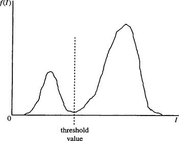
Figure 4.1 Idealized histogram of pixel intensity levels in an image. The large peak on the right results from the light background; the smaller peak on the left is due to dark foreground objects. The minimum of the distribution provides a convenient intensity value to use as a threshold.
This method is subject to the following major difficulties:
1. The valley may be so broad that it is difficult to locate a significant minimum.
2. There may be a number of minima because of the type of detail in the image, and selecting the most significant one will be difficult.
3. Noise within the valley may inhibit location of the optimum position.
4. There may be no clearly visible valley in the distribution because noise may be excessive or because the background lighting may vary appreciably over the image.
5. Either of the major peaks in the histogram (usually that due to the background) may be much larger than the other, and this will then bias the position of the minimum.
6. The histogram may be inherently multimodal, making it difficult to determine which is the relevant thresholding level.
Perhaps the worst of these problems is the last: if the histogram is inherently multimodal, and we are trying to employ a single threshold, we are applying what is essentially an ad hoc technique to obtain a meaningful result. In general, such efforts are unlikely to succeed, and this is clearly a case where full image interpretation must be performed before we can be satisfied that the results are valid. Ideally, thresholding rules have to be formed after many images have been analyzed. In what follows, such problems of meaningfulness are eschewed. Instead attention is concentrated on how best to find a genuine single threshold when its position is obscured, as suggested by problems (1)-(6) above (which can be ascribed to image “clutter,” noise, and lighting variations).
4.3.2 Tackling the Problem of Bias in Threshold Selection
This subsection considers problem (5) above—that of eliminating the bias in the selection of thresholds that arises when one peak in the histogram is larger than the other. First, note that if the relative heights of the peaks are known, this effectively eliminates the problem, since the “fixed proportion” method of threshold selection outlined above can be used. However, this is not normally possible. A more useful approach is to prevent bias by weighting down the extreme values of the intensity distribution and weighting up the intermediate values in some way. To achieve this effect, note that the intermediate values are special in that they correspond to object edges. Hence, a good basic strategy is to find positions in the image where there are significant intensity gradients—corresponding to pixels in the regions of edges—and to analyze the intensity values of these locations while ignoring other points in the image.
To develop this strategy, consider the “scattergram” of Fig. 4.2. Here pixel properties are plotted on a 2-D map with intensity variation along one axis and intensity gradient magnitude variation along the other. Broadly speaking, three main populated regions are seen on the map: (1) a low-intensity, low-gradient region corresponding to the dark objects; (2) a high-intensity, low-gradient region corresponding to the background; and (3) a medium-intensity, high-gradient region corresponding to object edges (Panda and Rosenfeld, 1978). These three regions merge into each other, with the high-gradient region that corresponds to edges forming a path from the low-intensity to the high-intensity region. The fact that the three regions merge in this way gives a choice of methods for selecting intensity thresholds. The first choice is to consider the intensity distribution along the zero gradient axis, but this alternative has the same disadvantage as the original histogram method—namely, introducing a substantial bias. The second choice is that at high gradient, which means looking for a peak rather than a valley in the intensity distribution. The final choice is that at moderate values of gradient, which was suggested earlier as a possible strategy for avoiding bias.
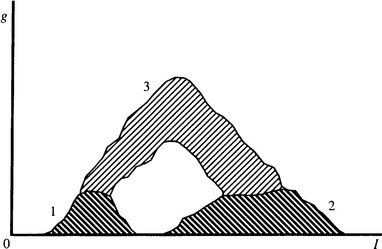
Figure 4.2 Scattergram showing the frequency of occurrence of various combinations of pixel intensity I and intensity gradient magnitude g in an idealized image. There are three main populated regions of interest: (1) a low I, low g region; (2) a high I, low g region; and (3) a medium I, high g region. Analysis of the scattergram provides useful information on how to segment the image.
It is now apparent that there is likely to be quite a narrow range of values of gradient for which the third method will be a genuine improvement. In addition, it may be necessary to construct a scattergram rather than a simple intensity histogram in order to locate it. If, instead, we try to weight the plots on a histogram with the magnitudes of the intensity gradient values, we are likely to end with a peaked intensity distribution (i.e., method 2) rather than one with a valley (Weska and Rosenfeld, 1979). A mathematical model of the situation is presented in Section 4.3.3 in order to explore the situation more fully.
4.3.2.1 Methods Based on Finding a Valley in the Intensity Distribution
This section considers how to weight the intensity distribution using a parameter other than the intensity gradient, in order to locate accurately the valley in the intensity distribution. A simple strategy is first to locate all pixels that have a significant intensity gradient and then to find the intensity histogram not only of these pixels but also of nearby pixels. This means that the two main modes in the intensity distribution are still attenuated very markedly and hence the bias in the valley position is significantly reduced. Indeed, the numbers of background and foreground pixels that are now being examined are very similar, so the bias from the relatively large numbers of background pixels is virtually eliminated. (Note that if the modes are modeled as two Gaussian distributions of equal widths and they also have equal heights, then the minimum lies exactly halfway between them.)
Though obvious, this approach includes the edge pixels themselves, and from Fig. 4.2 it can be seen that they will tend to fill the valley between the two modes. For the best results, the points of highest gradient must actually be removed from the intensity histogram. A well-attested way of achieving this is to weight pixels in the intensity histogram according to their response to a Laplacian filter (Weska et al., 1974). Since such a filter gives an isotropic estimate of the second derivative of the image intensity (i.e., the magnitude of the first derivative of the intensity gradient), it is zero where intensity gradient magnitude is high. Hence, it gives such locations zero weight, but it nevertheless weights up those locations on the shoulders of edges. It has been found that this approach is excellent at estimating where to place a threshold within a wide valley in the intensity histogram (Weska et al., 1974). Section 4.3.3 shows that this is far from being an ad hoc solution to a tedious problem. Rather, it is in many ways ideal in giving a very exact indication of the optimum threshold value.
4.3.2.2 Methods That Concentrate on the Peaked Intensity Distribution at High Gradient
The other approach indicated earlier is to concentrate on the peaked intensity distribution at high-gradient values. It seems possible that location of a peak will be less accurate (for the purpose of finding an effective intensity threshold value) than locating a valley between two distributions, especially when edges do not have symmetrical intensity profiles. However, an interesting result was obtained by Kittler et al. (1984, 1985), who suggested locating the threshold directly (i.e., without constructing an intensity histogram or a scattergram) by calculating the statistic:
where Ii is the local intensity and gi is the local intensity gradient magnitude. This statistic was found to be biased by noise, resulting in noisy background and foreground pixels that contributed to the average value of intensity in the threshold calculation. This effect occurs only if the image contains different numbers of background and foreground pixels. It is a rather different manifestation of the bias between the two histogram modes that was noted earlier. In this case, a formula including bias was obtained in the form
where T0 is the inherent (i.e., unbiased) threshold, C is the image contrast, and b is the proportion of background pixels in the image.
To understand the reasoning behind this formula, denote the background and foreground intensities as B and F, respectively, and the proportions of background and foreground pixels as b and f, where f + b = 1. (Here we are effectively assuming that a negligible proportion of pixels are situated on object edges. This is a reasonable assumption as the number of foreground and background pixels will be of order N2 for an N × N pixel image, whereas the number of edge pixels will be of order N.) Assuming a simple model of intensity variation, we find that
and
 (4.5)
(4.5)Equation (4.5) can be interpreted as follows. The threshold T is here calculated by averaging the intensity over image pixels, after weighting them in proportion to the local intensity gradient. Within the background, the pixels with appreciable intensity gradient are noise pixels, and these are proportional in number to b and have mean intensity B. Similarly, within the foreground, pixels with appreciable intensity gradient are proportional in number to fand have mean intensity F. As a result, the mean intensity of all these noise pixels is Bb + Ff, which is in agreement with the above equation for T. On the other hand, if pixels with low-intensity gradient are excluded, this progressively eliminates normal noise pixels and weights up the edge pixels (not represented in the above equation), so that the threshold reverts to the unbiased value T0. By applying the right corrections, Kittler et al. were able to eliminate the bias and to obtain a corrected threshold value T0 in practical situations, even when pixels with low-intensity gradient values were not excluded.
This method is useful because it results in unbiased estimates of the threshold T0 without the need to construct histograms or scattergrams. However, it is probably somewhat risky not to obtain histograms inasmuch as they give so much information—for example, on the existence of multiple modes. Thus, the statistic T may in complex cases amount to a bland average, which means very little. Ultimately, it seems that the safest threshold determination procedure must involve seeking and identifying specific peaks on the intensity histogram for relatively high values of intensity gradient, or specific troughs for relatively low values of intensity gradient.
4.3.3 A Convenient Mathematical Model
To get a clearer understanding of these problems, it is useful to construct a theoretical model of the situation. It is assumed that a number of dark, fairly flat objects are lying on a light worktable and are subject to soft, reasonably uniform lighting. In the absence of noise and other perturbations, the only variations in intensity occur near object boundaries (Fig. 2.3). With little loss of generality, the model can be simplified to a single dimension. It is easy to see that the distribution of intensities in the image is then as shown in Fig. 4.3 and is closely related to the shape of the edge profile. The intensity distribution is effectively the derivative of the edge profile:
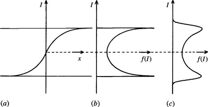
Figure 4.3 Relation of edge profile to intensity distribution: (a) shape of a typical edge profile; (b) resulting distribution of intensities; (c) effect of applying a broadening convolution (e.g., resulting from noise) to (b).
since for I in a given range ΔI, f (I) ΔI is proportional to the range of distances Ax that contribute to it. Taking account now of the fact that the entire image may contain many edges at specific locations, we can calculate the distribution f(I)in principle for all values of I, including the two very large peaks at the maximum and minimum values of intensity.
So far the model is incomplete in that it takes no account of noise or other variations in intensity. Essentially, these act in such a way as to broaden the intensity values from those predicted from edge profiles alone. This means that they can be allowed for by applying a broadening convolution b(I)to f(I):
This gives the more realistic distribution shown in Fig. 4.3c. These ideas confirm that a high histogram peak at the highest or lowest value of intensity can pull the minimum one way or the other and result in the original automatic threshold selection criterion being inaccurate.
In what follows, we simplify the analysis by returning to the unbroadened distributionf(I). We make the following definitions of intensity gradient g and rate of change of intensity gradient g’:
Applying equation (4.6), we find that
If we wish to weight the contributions to f(I) using some power p of |g|, the new distribution becomes:
This is not a sharp unimodal distribution as required by the earlier discussion, unless p > 1. We could conveniently set p = 2, although in practice workers have sometimes opted for a nonlinear, sharply varying weighting which is unity if |g| exceeds a given threshold and zero otherwise (Weska and Rosenfeld, 1979). This matter is not pursued further here. Instead, we consider the effect of weighting the contributions to f(I) using |g’| and obtain the new distribution:
Applying equations (4.6) and (4.9) now gives
To proceed further, an exact mathematical model is needed. A convenient one is obtained using the tanh function:
with I being restricted to the range—I0 ≤ I ≤ I0. (Note that we have simplified the model by making I zero at the center of the range.) This leads to:
 (4.15)
Applying equation (4.8)-(4.9) now gives
and
Note that the form of g given by the model, as a function of x, is:
Although a Gaussian variation for g might fit real data better, the present model has the advantage of simplicity and is able to provide useful insight into the problem of thresholding.
Applying equation (4.10)-(4.13) and (4.16), we may deduce that
We have now arrived at an interesting point: starting with a particular edge profile, we have calculated the shape of the basic intensity distribution f(I), the shape of the intensity distribution h(I) resulting from weighting pixel contributions according to a power of the intensity gradient value, and the distribution k(I) resulting from weighting them according to the spatial derivative of the intensity gradient, that is, according to the output of a Laplacian operator. The k(I) distribution has a very sharp valley with linear variation near the minimum. By contrast, h(I) varies rather slowly and smoothly near its maximum. This shows that the Laplacian weighting method should provide the most sensitive indicator of the optimum threshold value and thereby provides strong justification for the use of this method. However, it must be made absolutely clear that the advantages of this approach may well be washed away in practice if the assumptions made in the model are invalid. In particular, broadening of the distribution by noise, variations in background lighting, image clutter, and other artifacts will affect the situation adversely for all of the above methods. Further detailed analysis seems pointless, in part because these interfering factors make choice of the threshold more difficult in a very data-dependent way, but more importantly because they ultimately make the concept of thresholding at a single level invalid (see Figs 4.4-4.6).
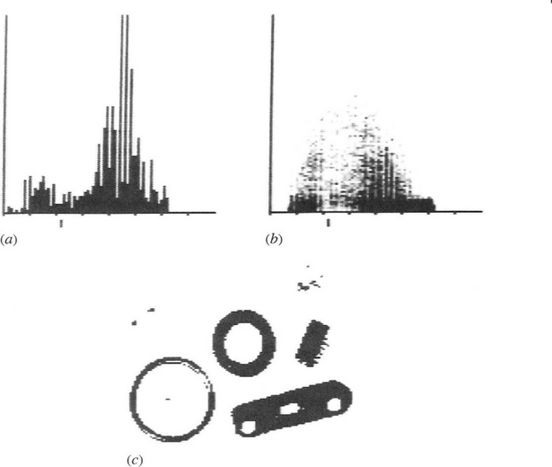
Figure 4.4 (a) Histogram and (b) scattergram for the image shown in Fig. 2.11a. In neither case is the diagram particularly close to the ideal form of Figs. 4.1 and 4.2. Hence, the threshold obtained from (a) (indicated by the short lines beneath the two scales) does not give ideal results with all the objects in the binarized image (c). Nevertheless, the results are better than for the arbitrarily thresholded image of Fig. 2.11.b.
4.3.4 Summary
It has been shown that available techniques can provide values at which intensity thresholding can be applied, but they do not themselves solve the problems caused by uneven lighting. They are even less capable of coping with glints, shadows, and image clutter. Unfortunately, these artifacts are common in most real situations and are only eliminated with difficulty. Indeed, in industrial applications where shiny metal components are involved, glints are the rule rather than the exception, whereas shadows can seldom be avoided with any sort of object. Even flat objects are liable to have quite a strong shadow contour around them because of the particular placing of lights. Lighting problems are studied in detail in Chapter 27. Meanwhile, it may be noted that glints and shadows can only be allowed for properly in a two-stage image analysis system, where tentative assignments are made first and these are firmed up by exact explanation of all pixel intensities. We now return to the problem of making the most of the thresholding technique—by finding how we can allow for variations in background lighting.
4.4 Adaptive Thresholding
The problem that arises when illumination is not sufficiently uniform may be tackled by permitting the threshold to vary adaptively (or “dynamically”) over the whole image. In principle, there are several ways of achieving this. One involves modeling the background within the image. Another is to work out a local threshold value for each pixel by examining the range of intensities in its neighborhood. A third approach is to split the image into subimages and deal with them independently. Though “obvious,” this last method will clearly run into problems at the boundaries between subimages, and by the time these problems have been solved it will look more like one of the other two methods. Ultimately, all such methods must operate on identical principles. The differences arise in the rigor with which the threshold is calculated at different locations and in the amount of computation required in each case. In real-time applications the problem amounts to finding how to estimate a set of thresholds with a minimum amount of computation.
The problem can sometimes be solved rather neatly in the following way. On some occasions—such as in automated assembly applications—it is possible to obtain an image of the background in the absence of any objects. This appears to solve the problem of adaptive thresholding in a rigorous manner, since the tedious task of modeling the background has already been carried out. However, some caution is needed with this approach. Objects bring with them not only shadows (which can in some sense be regarded as part of the objects), but also an additional effect due to the reflections they cast over the background and other objects. This additional effect is nonlinear, in the sense that it is necessary to add not only the difference between the object and the background intensity in each case but also an intensity that depends on the products of the reflectances of pairs of objects. These considerations mean that using the no-object background as the equivalent background when several objects are present is ultimately invalid. However, as a first approximation it is frequently possible to assume an equivalence. If this proves impracticable, the only option is to model the background from the actual image to be segmented.
On other occasions, the variation in background intensity may be rather slowly varying, in which case it may be possible to model it by the following technique. (this is a form of Hough transform—see Chapter 9.) First, an equation is selected which can act as a reasonable approximation to the intensity function, for example, a linear or quadratic variation:
Next, a parameter space for the six variables a, b, c, d, e, fis constructed. Then each pixel in the image is taken in turn, and all sets of values of the parameters that could have given rise to the pixel intensity value are accumulated in parameter space. Finally, a peak is sought in parameter space which represents an optimal fit to the background model. So far it appears that this has been carried out only for a linear variation, the analysis being simplified initially by considering only the differences in intensities of pairs of points in image space (Nixon, 1985). Note that a sufficient number of pairs of points must be considered so that the peak in parameter space resulting from background pairs is sufficiently well populated. This implies quite a large computational load for quadratic or higher variations in intensity. Hence, it is unlikely that this method will be generally useful if the background intensity is not approximated well by a linear variation.
4.4.1 The Chow and Kaneko Approach
As early as 1972, Chow and Kaneko introduced what is widely recognized as the standard technique for dynamic thresholding. It performs a thoroughgoing analysis of the background intensity variation, making few compromises to save computation (Chow and Kaneko, 1972). In this method, the image is divided into a regular array of overlapping subimages, and individual intensity histograms are constructed for each one. Those that are unimodal are ignored since they are assumed not to provide any useful information that can help in modeling the background intensity variation. However, the bimodal distributions are well suited to this task. These are individually fitted to pairs of Gaussian distributions of adjustable height and width, and the threshold values are located. Thresholds are then found, by interpolation, for the unimodal distributions. Finally, a second stage of interpolation is necessary to find the correct thresholding value at each pixel.
One problem with this approach is that if the individual subimages are made very small in an effort to model the background illumination more exactly, the statistics of the individual distributions become worse, their minima become less well defined, and the thresholds deduced from them are no longer statistically significant. This means that it does not pay to make subimages too small and that ultimately only a certain level of accuracy can be achieved in modeling the background in this way. The situation is highly data dependent, but little can be expected to be gained by reducing the subimage size below 32 × 32 pixels. Chow and Kaneko employed 256 × 256 pixel images and divided these into a 7 × 7 array of 64 × 64 pixel subimages with 50% overlap.
Overall, this approach involves considerable computation, and in real-time applications it may well not be viable for this reason. However, this type of approach is of considerable value in certain medical, remote sensing, and space applications. In addition, note that the method of Kittler et al. (1985) referred to earlier may be used to obtain threshold values for the subimages with rather less computation.
4.4.2 Local Thresholding Methods
In real-time applications the alternative approach mentioned earlier is often more useful for finding local thresholds. It involves analyzing intensities in the neighborhood of each pixel to determine the optimum local thresholding level. Ideally, the Chow and Kaneko histogramming technique would be repeated at each pixel, but this would significantly increase the computational load of this already computationally intensive technique. Thus, it is necessary to obtain the vital information by an efficient sampling procedure. One simple means of achieving this is to take a suitably computed function of nearby intensity values as the threshold. Often the mean of the local intensity distribution is taken, since this is a simple statistic and gives good results in some cases. For example, in astronomical images stars have been thresholded in this way. Niblack (1985) reported a case in which a proportion of the local standard deviation was added to the mean to give a more suitable threshold value, the reason (presumably) being to help suppress noise. (Addition is appropriate where bright objects such as stars are to be located, whereas subtraction will be more appropriate in the case of dark objects.)
Another frequently used statistic is the mean of the maximum and minimum values in the local intensity distribution. Whatever the sizes of the two main peaks of the distribution, this statistic often gives a reasonable estimate of the position of the histogram minimum. The theory presented earlier shows that this method will only be accurate if (1) the intensity profiles of object edges are symmetrical, (2) noise acts uniformly everywhere in the image so that the widths of the two peaks of the distribution are similar, and (3) the heights of the two distributions do not differ markedly. Sometimes these assumptions are definitely invalid—for example, when looking for (dark) cracks in eggs or other products. In such cases the mean and maximum of the local intensity distribution can be found, and a threshold can be deduced using the statistic
where the strategy is to estimate the lowest intensity in the bright background assuming the distribution of noise to be symmetrical (Fig. 4.7). Use of the mean here is realistic only if the crack is narrow and does not affect the value of the mean significantly. If it does, then the statistic can be adjusted by use of an ad hoc parameter:
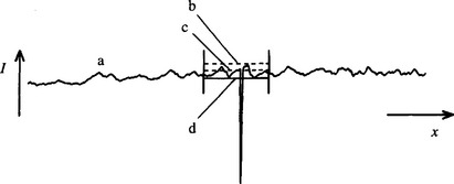
Figure 4.7 Method for thresholding the crack in an egg. (a) Intensity profile of an egg in the vicinity of a crack: the crack is assumed to appear dark (e.g., under oblique lighting); (b) local maximum of intensity on the surface of the egg; (c) local mean intensity. Equation (4.24) gives a useful estimator T of the thresholding level (d).
where k may be as low as 0.5 (Plummer and Dale, 1984).
This method is essentially the same as that of Niblack (1985), but the computational load in estimating the standard deviation is minimized. Each of the last two techniques relies on finding local extrema of intensity. Using these measures helps save computation, but they are somewhat unreliable because of the effects of noise. If this is a serious problem, quartiles or other statistics of the distribution may be used. The alternative of prefiltering the image to remove noise is unlikely to work for crack thresholding because cracks will almost certainly be removed at the same time as the noise. A better strategy is to form an image of T-values obtained using equation (4.24) or (4.25). Smoothing this image should then permit the initial image to be thresholded effectively.
Unfortunately, all these methods work well only if the size of the neighborhood selected for estimating the required threshold is sufficiently large to span a significant amount of foreground and background. In many practical cases, this is not possible and the method then adjusts itself erroneously, for example, so that it finds darker spots within dark objects as well as segmenting the dark objects themselves. However, in certain applications there is little risk of this occurring. One notable case is that of OCR. Here the widths of character limbs are likely to be known in advance and should not vary substantially. If this is so, then a neighborhood size can be chosen to span or at least sample both character and background. It is thus possible to threshold the characters highly efficiently using a simple functional test of the type described above. The effectiveness ofthis procedure (Fig. 4.8) is demonstrated in Fig. 4.9.
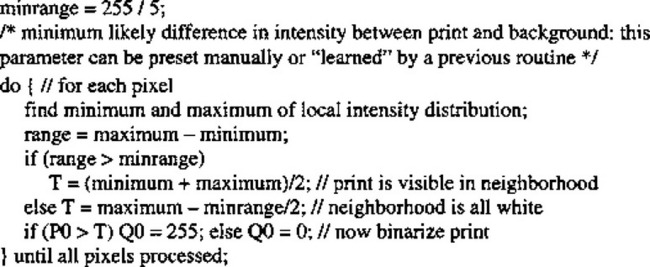
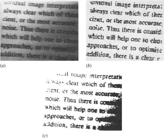
Figure 4.9 Effectiveness of local thresholding on printed text. Here a simple local thresholding procedure (Fig. 4.8), operating within a 3 × 3 neighborhood, is used to binarize the image of a piece of printed text (a). Despite the poor illumination, binarization is performed quite effectively (b). Note the complete absence of isolated noise points in (b), while by contrast the dots on all the i’s are accurately reproduced. The best that could be achieved by uniform thresholding is shown in (c).
Finally, before leaving this topic, it should be noted that hysteresis thresholding is a type of adaptive thresholding—effectively permitting the threshold value to vary locally. This topic will be investigated in Section 7.1.1.
4.5 More Thoroughgoing Approaches to Threshold Selection
At this point, we return to global threshold selection and describe some especially important approaches that have a rigorous mathematical basis. The first of these approaches is variance-based thresholding; the second is entropy-based thresholding; and the third is maximum likelihood thresholding. All three are widely used, the second having achieved an increasingly wide following over the past 20 to 30 years. The third is a more broadly based technique that has its roots in statistical pattern recognition—a subject that is dealt with in depth in Chapter 24.
4.5.1 Variance-based Thresholding
The standard approach to thresholding outlined earlier involved finding the neck of the global image intensity histogram. However, this is impracticable when the dark peak of the histogram is minuscule in size, for it will then be hidden among the noise in the histogram and it will not be possible to extract it with the usual algorithms.
Many investigators have studied this problem (e.g., Otsu, 1979; Kittler et al., 1985; Sahoo et al., 1988; Abutaleb, 1989). Among the most well-known approaches are the variance-based methods. In these methods, the image intensity histogram is analyzed to find where it can best be partitioned to optimize criteria based on ratios of the within-class, between-class, and total variance. The simplest approach (Otsu, 1979) is to calculate the between-class variance, as will now be described.
First, we assume that the image has a gray-scale resolution of L gray levels. The number of pixels with gray level i is written as ni, so the total number of pixels in the image is N = n1 + n2 + … +nL. Thus, the probability of a pixel having gray level i is:
where
For ranges of intensities up to and above the threshold value k, we can now calculate the between-class variance σ2B and the total variance σ2T:
where
 (4.30)
 (4.31)
Making use of the latter definitions, the formula for the between-class variance can be simplified to:
For a single threshold the criterion to be maximized is the ratio of the between-class variance to the total variance:
However, the total variance is constant for a given image histogram; thus, maximizing η simplifies to maximizing the between-class variance.
The method can readily be extended to the dual threshold case 1 ≤ k1 ≤ k2 ≤ L, where the resultant classes, C0, C1, and C2, have respective gray-level ranges of [1,…, k1], [k1 + 1,…, k2], and [k2 + 1,…, L].
In some situations (e.g., Hannah et al., 1995), this approach is still not sensitive enough to cope with histogram noise, and more sophisticated methods must be used. One such technique is that of entropy-based thresholding, which has become firmly embedded in the subject (Pun, 1980; Kapur et al., 1985; Abutaleb, 1989; Brink, 1992).
4.5.2 Entropy-based Thresholding
Entropy measures of thresholding are based on the concept of entropy. The entropy statistic is high if a variable is well distributed over the available range, and low if it is well ordered and narrowly distributed. Specifically, entropy is a measure of disorder and is zero for a perfectly ordered system. The concept of entropy thresholding is to threshold at an intensity for which the sum of the entropies of the two intensity probability distributions thereby separated is maximized. The reason for this is to obtain the greatest reduction in entropy—that is, the greatest increase in order—by applying the threshold. In other words, the most appropriate threshold level is the one that imposes the greatest order on the system, and thus leads to the most meaningful result.
To proceed, the intensity probability distribution is again divided into two classes—those with gray levels up to the threshold value k, and those with gray levels above k (Kapur et al., 1985). This leads to two probability distributions A and B:
where
 (4.36)
The entropies for each class are given by
 (4.37)
 (4.38)
Substitution leads to the final formula:
 (4.40)
and it is this parameter that has to be maximized.
This approach can give very good results—see, for example, Hannah et al. (1995). Again, it is straightforwardly extended to dual thresholds, but we shall not go into the details here (Kapur et al., 1985). Probabilistic analysis to find mathematically ideal dual thresholds may not be the best approach in practical situations. An alternative technique for determining dual thresholds sequentially has been devised by Hannah et al. (1995) and applied to an X-ray inspection task—as described in Chapter 22.
4.5.3 Maximum Likelihood Thresholding
When dealing with distributions such as intensity histograms, it is important to compare the actual data with the data that might be expected from a previously constructed model based on a training set. This is in keeping with the methods of statistical pattern recognition (see Chapter 24), which takes full account of prior probabilities. For this purpose, one option is to model the training set data using a known distribution function such as a Gaussian. The Gaussian model has many advantages, including its accessibility to relatively straightforward mathematical analysis. In addition, it is specifiable in terms of two well-known parameters—the mean and standard deviation—which are easily measured in practical situations. Indeed, for any Gaussian distribution we have:
where the suffix i refers to a specific distribution, and of course when thresholding is being carried out two such distributions are assumed to be involved. Applying the respective a priori class probabilities P1, P2 (Chapter 24), careful analysis (Gonzalez and Woods, 1992) shows that the condition p1(x)= p2(x) reduces to the form:
Note that, in general, this equation has two solutions,2implying the need for two thresholds, though when a1 = a2 there is a single solution:
In addition, when the prior probabilities for the two classes are equal, the equation reduces to the altogether simpler and more obvious form:
Of all the methods described in this chapter, only the maximum likelihood method makes use of a priori probabilities. Although this makes it appear to be the only rigorous method, and indeed that all other methods are automatically erroneous and biased in their estimations, this need not be the actual position. The reason lies in the fact that the other methods incorporate actual frequencies of sample data, which should embody the a priori probabilities (see Section 2.4.4). Hence, the other methods could well give correct results. Nevertheless, it is refreshing to see a priori probabilies brought in explicitly, for this gives a greater confidence of getting unbiased results in any doubtful situations.
4.6 Concluding Remarks
A number of factors are crucial to the process of thresholding: first, the need to avoid bias in threshold selection by arranging roughly equal populations in the dark and light regions of the intensity histogram; second, the need to work with the smallest possible subimage (or neighborhood) size so that the intensity histogram has a well-defined valley despite variations in illumination; and third, the need for subimages to be sufficiently large so that statistics are good, permitting the valley to be located with precision.
A moment s thought will confirm that these conditions are not compatible and that a definite compromise will be needed in practical situations. In particular, it is generally not possible to find a neighborhood size that can be applied everywhere in an image, on all occasions yielding roughly equal populations of dark and light pixels. Indeed, if the chosen size is small enough to span edges ideally, hence yielding unbiased local thresholds, it will be totally at a loss inside large objects. Attempting to avoid this situation by resorting to alternative methods of threshold calculation—as for the statistic of equation (4.1)—does not solve the problem since inherent in such methods is a built-in region size. (In equation (4.1) the size is given by the summation limits.) It is therefore not surprising that a number of workers have opted for variable resolution and hierarchical techniques in an attempt to make thresholding more effective (Wu et al., 1982; Wermser et al., 1984; Kittler et al., 1985).
At this stage we call to question the complications involved in such thresholding procedures—which become even worse when intensity distributions start to become multimodal. Note that the overall procedure is to find local intensity gradients in order to obtain accurate, unbiased estimates ofthresholds, so that it then becomes possible to take a horizontal slice through a grey-scale image and hence, ultimately, find “vertical” (i.e., spatial) boundaries within the image. Why not use the gradients directly to estimate the boundary positions? Such an approach, for example, leads to no problems from large regions where intensity histograms are essentially unimodal, although it would be foolish to pretend that no other problems exist (see Chapters 5 and 7).
On the whole, many approaches (region-growing, thresholding, edge detection, etc.), taken to the limits of approximation, will give equally good results. After all, they are all limited by the same physical effects—image noise, variability of lighting, the presence of shadows, and so on. However, some methods are easier to coax into working well, or need minimal computation, or have other useful properties such as robustness. Thus, thresholding can be a highly efficient means of aiding the interpretation of certain types of images, but as soon as image complexity rises above a certain critical level, it suddenly becomes more effective and considerably less complicated to employ overt edge detection techniques. These techniques are studied in depth in the next chapter. Meanwhile, we must not overlook the possibility of easing the thresholding process by going to some trouble to optimize the lighting system and to ensure that any worktable or conveyor is kept clean and white. This turns out to be a viable approach in a surprisingly large number of industrial applications.
The end result of thresholding is a set of silhouettes representing the shapes of objects, these constitute a “binarized” version of the original image. Many techniques exist for performing binary shape analysis, and some of these are described in Chapter 6. Meanwhile, it should be noted that many features of the original scene—for example, texture, grooves, or other surface structure—will not be present in the binarized image. Although the use of multiple thresholds to generate a number of binarized versions of the original image can preserve relevant information present in the original image, this approach tends to be clumsy and impracticable, and sooner or later one is likely to be forced to return to the original gray-scale image for the required data.
Thresholding is among the simplest of image processing operations and is an intrinsically appealing way of performing segmentation. This chapter has shown that even with the most scientific means of determining thresholds, it is a limited technique and can only form one of many tools in the programmer’s toolkit.
4.7 Bibliographical and Historical Notes
Segmentation by thresholding started many years ago from simple beginnings and in recent years has been refined into a set of mature procedures. In some ways these may have been pushed too far, or at least further than the basic concepts—which were after all intended to save computation—can justify. For example, Milgram’s (1979) method of “convergent evidence” works by trying many possible threshold values and finding iteratively which of these is best at making thresholding agree with the results of edge detection—a method involving considerable computation. Pal et al. (1983) devised a technique based on fuzzy set theory, which analyzes the consequences of applying all possible threshold levels and minimizes an “index of fuzziness.” This technique also has the disadvantage of large computational cost. The gray-level transition matrix approach of Deravi and Pal (1983) involves constructing a matrix of adjacent pairs of image intensity levels and then seeking a threshold within this matrix. This achieves the capability for segmentation even in cases where the intensity distribution is unimodal but with the disadvantage of requiring large storage space.
The Chow and Kaneko method (1972) has been seen to involve considerable amounts of processing (though Greenhill and Davies, 1995, have sought to reduce it with the aid of neural networks). Nakagawa and Rosenfeld (1979) studied the method and developed it for cases of trimodal distributions but without improving computational load. For bimodal distributions, however, the approach of Kittler et al. (1985) should require far less processing because it does not need to find a best fit to pairs of Gaussian functions.
Several workers have investigated the use of relaxation methods for threshold selection. In particular, Bhanu and Faugeras (1982) devised a gradient relaxation scheme that is useful for unimodal distributions. However, relaxation methods as a class are well known to involve considerable amounts ofcomputation even if they converge rapidly, since they involve several iterations of whole-image operations (see also Section 15.6). Indeed, in relation to the related region-growing approach, Fu and Mui (1981) stated explicitly that: “All the region extraction techniques process the pictures in an iterative manner and usually involve a great expenditure in computation time and memory. Finally, Wang and Haralick (1984) developed a recursive scheme for automatic multithreshold selection, which involves successive analysis of the histograms of relatively dark and relatively light edge pixels.
Fu and Mui (1981) provided a useful general survey on image segmentation, which has been updated by Haralick and Shapiro (1985). These papers review many topics that could not be covered in the present chapter for reasons of space and emphasis. A similar comment applies to Sahoo et al. s (1988) survey of thresholding techniques.
As hinted in Section 4.4, thresholding (particularly local adaptive thresholding) has had many applications in optical character recognition. Among the earliest were the algorithms described by Bartz (1968) and Ullmann (1974): two highly effective algorithms have been described by White and Rohrer (1983).
During the 1980s, the entropy approach to automatic thresholding evolved (e.g., Pun, 1981; Kapur et al., 1985; Abutaleb, 1989; Pal and Pal, 1989). This approach (Section 4.5.2) proved highly effective, and its development continued during the 1990s (e.g., Hannah et al., 1995). Indeed, it may surprise the reader that thresholding and adaptive thresholding are still hot subjects (see for example Yang et al., 1994; Ramesh et al., 1995).
Most recently, the entropy approach to threshold selection has remained important, in respect to both conventional region location and ascertaining the transition region between objects and background to make the segmentation process more reliable (Yan et al., 2003). In one instance it was found useful to employ fuzzy entropy and genetic algorithms (Tao et al., 2003). Wang and Bai (2003) have shown how threshold selection may be made more reliable by clustering the intensities of boundary pixels, while ensuring that a continuous rather than a discrete boundary is considered (the problem being that in images that approximate to binary images over restricted regions, the edge points will lie preferentially in the object or the background, not neatly between both). However, it has to be said that in complex outdoor scenes and for many medical images such as brain scans, thresholding alone will not be sufficient, and resort may even have to be made to graph matching (Chapter 15) to produce the best results—reflecting the important fact that segmentation is necessarily a high-level rather than a low-level process (Wang and Siskind, 2003). In rather less demanding cases, deformable model-guided split-and-merge techniques may, on the other hand, still be sufficient (Liu and Sclaroff, 2004).
4.8 Problems
1. Using the methods of Section 4.3.3, model the intensity distribution obtained by finding all the edge pixels in an image and including also all pixels adjacent to these pixels. Show that while this gives a sharper valley than for the original intensity distribution, it is not as sharp as for pixels located by the Laplacian operator.
2. Because of the nature of the illumination, certain fairly flat objects are found to have a fine shadow around a portion of their boundary. Show that this could confuse an adaptive thresholder that bases its threshold value on the statistic of equation (4.1).
3. Consider whether it is more accurate to estimate a suitable threshold for a bimodal, dual-Gaussian distribution by (a) finding the position of the minimum or (b) finding the mean of the two peak positions. What corrections could be made by taking account of the magnitudes of the peaks?
4. Obtain a complete derivation of equation (4.42). Show that, in general (as stated in Section 4.5.3), it has two solutions. What is the physical reason for this? How can it have only one solution when σ1 = σ2?
1 The danger is clearly that even one small break will in principle join two regions into a single larger one.
2 Two solutions exist because one solution represents a threshold in the area of overlap between the two Gaussians; the other solution is necessary mathematically and lies either at very high or very low intensities. It is the latter solution that disappears when the two Gaussians have equal variance, as the distributions clearly never cross again. In any case, it seems unlikely that the distributions being modeled would in practice approximate so well to Gaussians that the noncentral solution could ever be important—that is, it is essentially a mathematical fiction that needs to be eliminated from consideration.