7.1 Introduction

An earlier chapter showed how thresholding may be used to binarize gray-scale images and hence to present objects as 2-D shapes. This method of segmenting objects is successful only when considerable care is taken with lighting and when the object can be presented conveniently, for example, as dark patches on a light background. In other cases, adaptive thresholding may help to achieve the same end: as an alternative, edge detection schemes can be applied, these schemes generally being rather more resistant to problems of lighting. Nevertheless, thresholding of edge-enhanced images still poses certain problems; in particular, edges may peter out in some places and may be thick in others (Fig. 7.1). For many purposes, the output of an edge detector is ideally a connected unit-width line around the periphery of an object, and steps will need to be taken to convert edges to this form.

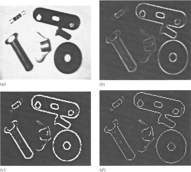
Figure 7.1 Some problems with edges. The edge-enhanced image (b) from an original image (a) is thresholded as in (c). The edges so detected are found to peter out in some places and to be thick in other places. A thinning algorithm is able to reduce the edges to unit thickness (d), but ad hoc (i.e., not model-based) linking algorithms are liable to produce erroneous results (not shown).

Thinning algorithms can be used to reduce edges to unit thickness, while maintaining connectedness (Fig. 7.1 d). Many algorithms have been developed for this purpose, and the main problems here are: (1) slight bias and inaccuracy due to uneven stripping of pixels, especially in view of the fact that even the best algorithm can only produce a line that is locally within 1/2 pixel of the ideal position; and (2) introduction of a certain number of noise spurs. The first of these problems can be minimized by using gray-scale edge thinning algorithms which act directly on the original gray-scale edge-enhanced image (e.g., Paler and Kittler, 1983). Noise spurs around object boundaries can be eliminated quite efficiently by removing lines that are shorter than (say) 3 pixels. Overall, the major problem to be dealt with is that of reconnecting boundaries that have become fragmented during thresholding.

A number of rather ad hoc schemes are available for relinking broken boundaries. For example, line ends may be extended along their existing directions—a very limited procedure since there are (at least for binary edges) only eight possible directions, and it is quite possible for the extended line ends not to meet. Another approach is to join line ends which are (1) sufficiently close together and (2) pointing in similar directions to each other and to the direction of the vector between the two ends. This approach can be made quite credible in principle, but in practice it can lead to all sorts of problems as it is still ad hoc and not model driven. Hence, adjacent lines that arise from genuine surface markings and from shadows may be arbitrarily linked together by such algorithms. In many situations it is therefore best if the process is model driven—for example, by finding the best fit to some appropriate idealized boundary such as an ellipse. Yet another approach is that of relaxation labeling, which iteratively enhances the original image, progressively making decisions as to where the original gray levels reinforce each other. Thus, edge linking is permitted only where evidence is available in the original image that this is permissible. A similar but computationally more efficient line of attack is the hysteresis thresholding method of Canny (1986). Here intensity gradients above a certain upper threshold are taken to give definite indication of edge positions, whereas those above a second, lower threshold are taken to indicate edges only if they are adjacent to positions that have already been accepted as edges (for a detailed analysis, see Section 7.1.1).

It may be thought that the Marr-Hildreth and related edge detectors do not run into these problems because they give edge contours that are necessarily connected. However, the result of using methods that force connectedness is that sometimes (e.g., when edges are diffuse, or of low contrast, so that image noise is an important factor) parts of a contour will lack meaning. Indeed, a contour may meander over such regions following noise rather than useful object boundaries. Furthermore, it is as well to note that the problem is not merely one of pulling low-level signals out of noise, but rather that sometimes no signal at all is present that could be enhanced to a meaningful level. One reason may be that the lighting is such as to give zero contrast (as, for example, when a cube is lit in such a way that two faces have equal brightness) and occlusion. Lack of spatial resolution can also cause problems by merging together several lines on an object.

It is now assumed that all of these problems have been overcome by sufficient care with the lighting scheme, appropriate digitization, and other means. It is also assumed that suitable thinning and linking algorithms have been applied so that all objects are outlined by connected unit-width boundary lines. At this stage, it should be possible (1) to locate the objects from the boundary image, (2) to identify and orient them accurately, and (3) to scrutinize them for shape and size defects.

7.1.1 Hysteresis Thresholding

The concept of hysteresis thresholding is a general one that can be applied in a range of applications, including both image and signal processing. The Schmitt trigger is a very widely used electronic circuit for converting a varying voltage into a pulsed (binary) waveform. In this latter case, there are two thresholds, and the input has to rise above the upper threshold before the output is allowed to switch on and has to fall below the lower threshold before the output is allowed to switch off. This gives considerable immunity against noise in the input waveform—far more than where the difference between the upper and lower switching thresholds is zero (the case of zero hysteresis), since then a small amount of noise can cause an undue amount of switching between the upper and lower output levels.

When the concept is applied in image processing, it is usually with regard to edge detection, in which case there is an analogous 1-D waveform to be negotiated around the boundary of an object—though as we shall see, some specifically 2-D complications arise. The basic rule is to threshold the edge at a high level and then to allow extension of the edge down to a lower level threshold, but only adjacent to points that have already been assigned edge status.

Figure 7.2 shows the results of making tests on the edge gradient image in Fig. 8.4b. Figures 7.2a and b show the result of thresholding at the upper and lower hysteresis levels, respectively, and Fig. 7.2c shows the result of hysteresis thresholding using these two levels. For comparison, Fig. 7.2d shows the effect of thresholding at a suitably chosen intermediate level. Note that isolated edge points within the object boundaries are ignored by hysteresis thresholding, though noise spurs can occur and are retained. We can envision the process of hysteresis thresholding in an edge image as the location of points that

1. form a superset of the upper threshold edge image.

2. form a subset of the lower threshold edge image.

3. form that subset of the lower threshold image which is connected to points in the upper threshold image via the usual rules of connectedness (Chapter 6).

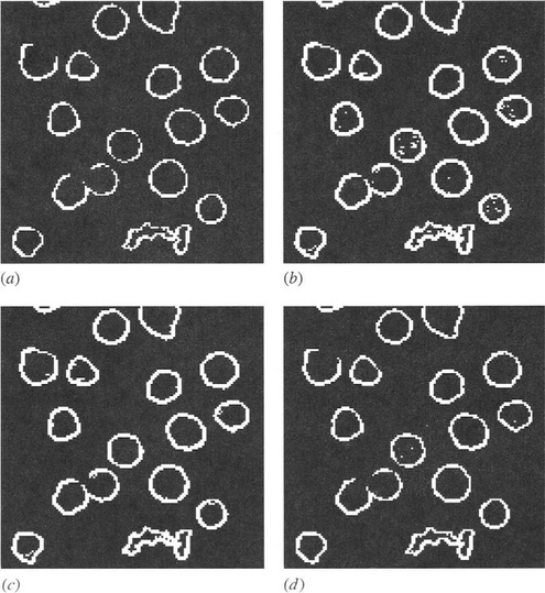
Figure 7.2 Effectiveness of hysteresis thresholding. This figure shows tests made on the edge gradient image of Fig. 8.4b.(a) Effect of thresholding at the upper hysteresis level. (b) Effect of thresholding at the lower hysteresis level. (c) Effect of hysteresis thresholding. (d) Effect of thresholding at an intermediate level.

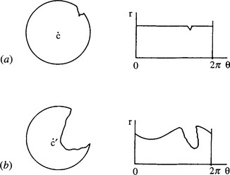
Figure 7.4 Effect of gross defects on the centroidal profile: (a) a chipped circular object and its centroidal profile; (b) a severely damaged circular object and its centroidal profile. The latter is distorted not only by the break in the circle but also by the shift in its centroid to C’.

Edge points survive only if they are seeded by points in the upper threshold image.

Although the result in Fig. 7.2c is better than in Fig. 7.2d, in that gaps in the boundaries are eliminated or reduced in length, in a few cases noise spurs are introduced. Nevertheless, the aim of hysteresis thresholding is to obtain a better balance between false positives and false negatives by exploiting connectedness in the object boundaries. Indeed, if managed correctly, the additional parameter will normally lead to a net (average) reduction in boundary pixel classification error. However, guidelines for selecting hysteresis thresholds are primarily the following:

1. Use a pair of hysteresis thresholds that provide immunity against the known range of noise levels.

2. Choose the lower threshold to limit the possible extent of noise spurs (in principle, the highest lower threshold whose subset contains all true boundary points).

3. Select the upper threshold to guarantee as far as possible the seeding of important boundary points (in principle, the highest upper threshold whose subset is connected to all true boundary points).

Unfortunately, in the limit of high signal variability, rules 2 and 3 appear to suggest eliminating hysteresis altogether! Ultimately, this means that the only rigorous way of treating the problem is to perform a complete statistical analysis of false positives and false negatives for a large number of images in any new application.

7.2 Boundary Tracking Procedures

Before objects can be matched from their boundary patterns, means must be found for tracking systematically around the boundaries of all the objects in an image. Means have already been demonstrated for achieving this in the case of regions such as those that result from intensity thresholding routines (Chapter 6). However, when a connected unit-width boundary exists, the problem oftracking is much simpler, since it is necessary only to move repeatedly to the next edge pixel storing the boundary information, for example, as a suitable pair of 1-D periodic coordinate arrays x[i], y[i]. Note that each edge pixel must be marked appropriately as we proceed around the boundary, to ensure (1) that we never reverse direction, (2) that we know when we have been around the whole boundary once, and (3) that we record which object boundaries have been encountered. As when tracking around regions, we must ensure that in each case we end by passing through the starting point in the same direction.

7.3 Template Matching—A Reminder

Before considering boundary pattern analysis, recall the object location problem discussed in Chapter 1. With 2-D images there is a significant matching problem because of the number of degrees of freedom involved. Usually, there will be two degrees of freedom for position and one for orientation. For an object of size 30 × 30 pixels in a 256 × 256 image, matching the position in principle requires some 256 × 256 trials, each one involving 30 × 30 operations. Since the orientation is generally also unknown, another factor of 360 is required to cope with varying orientation (i.e., one trial per degree of rotation), hence making a total of 256² × 30² × 360, that is, some 20,000 million operations. If more than one type of object is present, or if the objects have various possible scales, or if color variations have to be coped with,¹ the combinatorial explosion will be even more serious.

This is clearly an unacceptable situation, since even a modern computer could take several hours to locate objects within the image.

7.4 Centroidal Profiles

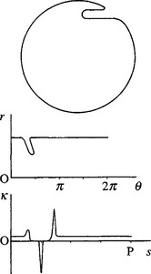
The matching problems outlined here make it attractive to attempt to locate objects in a smaller search space. This can be done simply by matching the boundary of each object in a single dimension. Perhaps the most obvious such scheme uses an (r, θ) plot. Here the centroid of the object is first located.² Then a polar coordinate system is set up relative to this point, and the object boundary is plotted as an (r, θ)graph—often called a centroidal profile (Fig. 7.3). Next, the 1-D graph so obtained is matched against the corresponding graph for an idealized object of the same type. Since the object in general has an arbitrary orientation, it is necessary to “slide” the idealized graph along that obtained from the image data until the best match is obtained. The match for each possible orientation α_j of the object is commonly tested by measuring the differences in radial distance between the boundary graph B and the template graph T for various values of 6 and summing their squares to give a difference measure Dj for the quality of the fit:

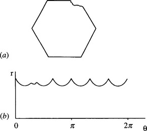
Figure 7.3 Centroidal profiles for object recognition and scrutiny: (a) hexagonal nut shape in which one corner has been damaged; (b) centroidal profile, which permits both straightforward identification of the object and detailed scrutiny of its shape.

     (7.1)

Alternatively, the absolute magnitudes of the differences are used:

     (7.2)

The latter measure has the advantage of being easier to compute and of being less biased by extreme or erroneous difference values. This factor of 360 referred to above still affects the amount of computation, but at least the basic 2-D matching operation is reduced to 1-D. Interestingly, the scale of the problem is reduced in two ways, since both the idealized template and the image data are now 1-D. In the above example, the result is that the number of operations required to test each object drops to around 360² (which is only about 100,000), so there is a very substantial saving in computation.

The 1-D boundary pattern matching approach is able to identify objects as well as to find their orientations. Initial location of the centroid of the object also solves one other part of the problem as specified at the end of Section 7.1. At this stage it may be noted that the matching process also leads to the possibility of inspecting the object’s shape as an inherent part of the process (Fig. 7.3). In principle, this combination of capabilities makes the centroidal profile technique quite powerful.

Finally, note that the method is able to cope with objects of identical shapes but different sizes. This is achieved by using the maximum value of r to normalize the profile, giving a variation (ρ, θ) where p = r/r_max.

7.5 Problems with the Centroidal Profile Approach

In practice, the procedure we have outlined poses several problems. First, any major defect or occlusion of the object boundary can cause the centroid to be moved away from its true position, and the matching process will be largely spoiled (Fig. 7.4). Thus, instead of concluding that this is an object of type × with a specific part of its boundary damaged, the algorithm will most probably not recognize it at all. Such behavior would be inadequate in many automated inspection applications, where positive identification and fault-finding are required, and the object would have to be rejected without a satisfactory diagnosis being made.

Second, the (r, θ)plot will be multivalued for a certain class of object (Fig. 7.5). This has the effect of making the matching process partly 2-D and leads to complication and excessive computation.

Figure 7.5 Boundary pattern analysis via (r, θ)and (s, κ) plots.

Third, the very variable spacing of the pixels when plotted in (r, θ) space is a source of complication. It leads to the requirement for considerable smoothing of the 1-D plots, especially in regions where the boundary comes close to the centroid—as for elongated objects such as spanners or screwdrivers (Fig. 7.6). However, in other places accuracy will be greater than necessary, and the overall process will be wasteful. The problem arises because quantization should ideally be uniform along the θ-axis so that the two templates can be moved conveniently relative to one another to find the orientation of best match.

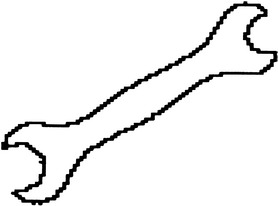
Figure 7.6 A problem in obtaining a centroidal profile for elongated objects. This figure highlights the pixels around the boundary of an elongated object—a spanner—showing that it will be difficult to obtain an accurate centroidal profile for the region near the centroid.

Finally, computation times can still be quite significant, so some timesaving procedure is required.

7.6 The (s, ψ) Plot

As can be seen from the above considerations, boundary pattern analysis should usually be practicable except when problems from occlusions and gross defects can be expected. These latter problems do give motivation, however, for employing alternative methods if these can be found. The (s, ψ) graph has proved especially popular since it is inherently better suited than the (r, θ)graph to situations where defects and occlusions may occur. In addition, it does not suffer from the multiple values encountered by the (r, θ) method.

The (s,ψ) graph does not require prior estimation of the centroid or some other reference point since it is computed directly from the boundary, in the form of a plot of the tangential orientation as a function of boundary distance s. The method is not without its problems, and, in particular, distance along the boundary needs to be measured accurately. The commonly used approach is to count horizontal and vertical steps as unit distance, and to take diagonal steps as distance . This idea must be regarded as a rather ad hoc solution; the situation is discussed further in Section 7.10.

When considering application of the (s,ψ) graph for object recognition, it will immediately be noticed that the graph has a ψ value that increases by 2π for each circuit of the boundary; that is, ψ(s) is not periodic in s. The result is that the graph becomes essentially 2-D; that is, the shape has to be matched by moving the ideal object template both along the s-axis and along the -axis directions. Ideally, the template could be moved diagonally along the direction of the graph. However, noise and other deviations of the actual shape relative to the ideal shape mean that in practice the match must be at least partly 2-D, hence adding to the computational load.

One way of tackling this problem is to make a comparison with the shape of a circle of the same boundary length P. Thus, an (s, Δψ) graph is plotted, which reflects the difference Δψ between the ψ expected for the shape and that expected for a circle of the same perimeter:

     (7.7)

This expression helps to keep the graph 1-D, since A automatically resets itself to its initial value after one circuit of the boundary (i.e., Δψis periodic in s).

Next it should be noticed that the Δψ(s) variation depends on the starting position where s = 0 and that this is randomly sited on the boundary. It is useful to eliminate this dependence, which may be done by subtracting from A its mean value μ. This gives the new variable:

     (7.8)

At this stage, the graph is completely 1-D and is also periodic, being similar in these respects to an (r, θ) graph. Matching should now reduce to the straightforward task of sliding the template along the (s) graph until a good fit is achieved.

At this point, there should be no problems as long as (1) the scale of the object is known and (2) occlusions or other disturbances cannot occur. Suppose next that the scale is unknown; then the perimeter P may be used to normalize the value of s. If, however, occlusions can occur, then no reliance can be placed on P for normalizing s, and hence the method cannot be guaranteed to work. This problem does not arise if the scale of the object is known, since a standard perimeter P_T can be assumed. However, the possibility of occlusion gives further problems that are discussed in the next section.

Another way in which the problem of nonperiodic ψ(s)can be solved is by replacing by its derivative dψ/ds. Then the problem of constantly expanding ψ(which results in its increasing by 2π after each circuit of the boundary) is eliminated—the addition of 2π to ψ does not affect dψ /ds locally, since d(ψ +2π)/ds = dψ/ds. It should be noticed that dψ/ds is actually the local curvature function κ(s)(see Fig. 7.5), so the resulting graph has a simple physical interpretation. Unfortunately, this version of the method has its own problems in that κapproaches infinity at any sharp corner. For industrial components, which frequently have sharp corners, this is a genuine practical difficulty and may be tackled by approximating adjacent gradients and ensuring that κintegrates to the correct value in the region of a corner (Hall, 1979).

Many workers take the (s, κ)graph idea further and expand κ(s)as a Fourier series:

     (7.9)

This results in the well-known Fourier descriptor method. In this method, shapes are analyzed in terms of a series of Fourier descriptor components that are truncated to zero after a sufficient number of terms. Unfortunately, the amount of computation involved in this approach is considerable, and the tendency is to approximate curves with relatively few terms. In industrial applications where computations have to be performed in real time, this can give problems, so it is often more appropriate to match to the basic (s, κ) graph. In this way, critical measurements between object features can be made with adequate accuracy in real time.

7.7 Tackling the Problems of Occlusion

Whatever means are used for tackling the problem of continuously increasing ψ, problems still arise when occlusions occur. However, the whole method is not immediately invalidated by missing sections of boundary as it is for the basic (r, θ) method. As noted above, the first effect of occlusions is that the perimeter of the object is altered, so P can no longer be used to indicate its scale. Hence, the scale has to be known in advance: this is assumed in what follows. Another practical result of occlusions is that certain sections correspond correctly to parts of the object, whereas other parts correspond to parts of occluding objects. Alternatively, they may correspond to unpredictable boundary segments where damage has occurred. Note that if the overall boundary is that of two overlapping objects, the observed perimeter P_B will be greater than the ideal perimeter P_T.

Segmenting the boundary between relevant and irrelevant sections is, a priori, a difficult task. However, a useful strategy is to start by making positive matches wherever possible and to ignore irrelevant sections—that is, try to match as usual, ignoring any section of the boundary that is a bad fit. We can imagine achieving a match by sliding the template T along the boundary B. However, a problem arises since T is periodic in s and should not be cut off at the ends of the range 0 < s < P_T. As a result, it is necessary to attempt to match over a length 2P_T. At first sight, it might be thought that the situation ought to be symmetrical between B and T. However, T is known in advance, whereas B is partly unknown, there being the possibility of one or more breaks in the ideal boundary into which foreign boundary segments have been included. Indeed, the positions of the breaks are unknown, so it is necessary to try matching the whole of T at all positions on B. Taking a length 2PT in testing for a match effectively permits the required break to arise in T at any relevant position (see Fig. 7.7).

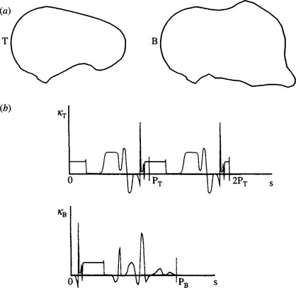
Figure 7.7 Matching a template against a distorted boundary. When a boundary B is broken (or partly occluded) but continuous, it is necessary to attempt to match between B and a template T that is doubled to length 2PT, to allow for T being severed at any point: (a) the basic problem; (b) matching in (s, k)-space.

When carrying out the match, we basically use the difference measure:

     (7.10)

where j and k are the match parameters for orientation and boundary displacement, respectively. Notice that the resulting D_jk is roughly proportional to the length L of the boundary over which the fit is reasonable. Unfortunately, this means that the measure D_jk appears to improve as L decreases. Hence, when variable occlusions can occur, the best match must be taken as the one for which the greatest length L gives good agreement between B and T. (This may be measured as the greatest number of values of s in the sum of equation (7.10) which give good agreement between B and T, that is, the sum over all i such that the difference in square brackets is numerically less than, say, 5^°.)

If the boundary is occluded in more than one place, then L is at most the largest single length of unoccluded boundary (not the total length of unoccluded boundary), since the separate segments will in general be “out of phase” with the template. This is a disadvantage when trying to obtain an accurate result, since extraneous matches add noise that degrades the fit that is obtainable—hence adding to the risk that the object will not be identified and reducing accuracy of registration. This suggests that it might be better to use only short sections of the boundary template for matching. Indeed, this strategy can be advantageous since speed is enhanced and registration accuracy can be retained or even improved by careful selection of salient features. (Note that nonsalient features such as smooth curved segments could have originated from many places on object boundaries and are not very helpful for identifying and accurately locating objects; hence it is reasonable to ignore them.) In this version of the method, we now have P_T < P_B, and it is necessary to match over a length P_T rather than 2P_T, since T is no longer periodic (Fig. 7.8). Once various segments have been located, the boundary can be reassembled as closely as possible into its full form, and at that stage defects, occlusions, and other distortions can be recognized overtly and recorded. Reassembly of the object boundaries can be performed by techniques such as the Hough transform and relational pattern matching techniques (see Chapters 11 and 15). Work of this type has been carried out by Turney et al. (1985), who found that the salient features should be short boundary segments where corners and other distinctive “kinks” occur.

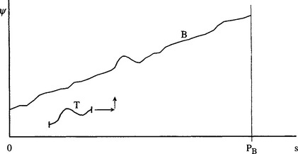
Figure 7.8 Matching a short template to part of a boundary. A short template T, corresponding to part of an idealized boundary, is matched against the observed boundary B. Strictly speaking, matching in (s, ψ)-space is 2-D, although there is very little uncertainty in the vertical (orientation) dimension.

It should be noted that ijr can no longer be used when occlusions are present, since although the perimeter can be assumed to be known, the mean value of Δψ (equation (7.8)) cannot be deduced. Hence, the matching task reverts to a 2-D search (though, as stated earlier, very little unrestrained search in the direction need be made). However, when small salient features are being sought, it is a reasonable working assumption that no occlusion occurs in any of the individual cases—a feature is either entirely present or entirely absent. Hence, the average slope ψ over T can validly be computed (Fig. 7.8), and this again reduces the search to 1-D (Turney et al., 1985).

Overall, missing sections of object boundaries necessitate a fundamental rethink as to how boundary pattern analysis should be carried out. For quite small defects, the (r, θ) method is sufficiently robust, but in less trivial cases it is vital to use some form of the (s,ψ) approach, while for really gross occlusions it is not particularly useful to try to match for the full boundary. Rather, it is better to attempt to match small salient features. This sets the scene for the Hough transform and relational pattern matching techniques of later chapters (see Parts 2 and 3).

7.8 Chain Code

This section briefly describes the chain code devised in 1961 by Herbert Freeman. This method recodes the boundary of a region into a sequence of octal digits, each one representing a boundary step in one of the eight basic directions relative to the current pixel position, denoted here by an asterisk:

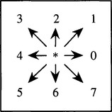
This code is important for presenting shape information in such a way as to save computer storage. In particular, note that the code ignores (and therefore does not store) the absolute position of the boundary pixels, so that only three bits are required for each boundary step. However, in order to regenerate a digital image, additional information is required, including the starting point of the chain and the length.

Chain code is useful in cutting down storage relative to the number of bits required to hold a list of the coordinates of all the boundary pixels (and a fortiori relative to the number of bits required to hold a whole binary image). In addition, chain code is able to provide data in a format that is suitable for certain recognition processes. However, chain coding may sometimes be too compressed a representation for convenient computer manipulation of the data. Hence, in many cases direct (x,y) storage may be more suitable, or otherwise direct (s,ψ) coding. Note also that with modern computers, the advantage of reduced storage requirements is becoming less relevant than in the early days of pattern recognition.

7.9 The (r, s) Plot

Before leaving the topic of 1-D plots for analysis and recognition of 2-D shapes, one further method should be mentioned—the (r, s)plot. Freeman (1978) introduced this method as a natural follow-up from the use of chain code (which necessarily involves the parameter s). Since quite a large family of possible 1-D plot representations exist, it is useful to demonstrate the particular advantages of any new one. The (r, s) plot is in many ways similar to the (r, θ) plot (particularly in using the centroid as a reference point) but it overcomes the difficulty of the (r, θ) plot sometimes being a multivalued function: for every value of s there is a unique value of r. However, against this advantage must be weighed the fact that it is not in general possible to recover the original shape from the 1-D plot, since an ambiguity is introduced whenever the tangent to the boundary passes through the centroid. To overcome this problem, a phase function Φ(s) (whose value is always either +1 or -1, the minus value corresponding to the curve turning back on itself) must be stored in addition to the function r(s). Freeman made a slight variation on this scheme by relying on the fact that r is always positive, so that all the information can be stored in a single function that is the product of r and Φ. Note, however, that the derived function is no longer continuous, so minor changes in shape could lead to misleadingly large changes in cross-correlation coefficient during comparison with a template.

7.10 Accuracy of Boundary Length Measures

Next we examine the accuracy of the idea expressed earlier—that adjacent pixels on an 8-connected curve should be regarded as separated by 1 pixel if the vector joining them is aligned along the major axes, and by pixels if the vector is in a diagonal orientation. It turns out that this estimator in general overestimates the distance along the boundary. The reason is quite simply seen by appealing to the following pair of situations:

In either case, we are considering only the top of the object. In the first example, the boundary length along the top of the object is exactly that given by the rule.

However, in the second case the estimated length is increased by amount −1 because of the step. Now as the length of the top of the object tends to large values, say p pixels, the actual length approximates to p while the estimated length is . Thus, a definite error exists. Indeed, this error initially increases in importance as p decreases, since the actual length of the top of the object (when there is one step) is still

     (7.11)

so the fractional error is

     (7.12)

which increases as p becomes smaller.

This result can be construed as meaning that the fractional error § in estimating boundary length increases initially as the boundary orientation increases from zero. A similar effect occurs as the orientation decreases from 45°. Thus, the § variation possesses a maximum between 0° and 45°. This systematic overestimation of boundary length may be eliminated by employing an improved model in which the length per pixel is s_m along the major axes directions and s_d in diagonal directions. A complete calculation (Kulpa, 1977; see also Dorst and Smeulders, 1987) shows that:

     (7.13)

and

     (7.14)

It is perhaps surprising that this solution corresponds to a ratio s_d/s_m that is still equal to , although the arguments given above make it obvious that s_m should be less than unity.

Unfortunately, an estimator that has just two free parameters can still permit quite large errors in estimating the perimeters of individual objects. To reduce this problem, it is necessary to perform more detailed modeling of the step pattern around the boundary (Koplowitz and Bruckstein, 1989), which seems certain to increase the computational load significantly.

It is important to underline that the basis of this work is to estimate the length of the original continuous boundary rather than that of the digitized boundary. Furthermore, it must be noted that the digitization process loses information, so the best that can be done is to obtain a best estimate of the original boundary length. Thus, employing the values 0.948, 1.343 given above, rather than the values 1, , reduces the estimated errors in boundary length measurement from 6.6% to 2.3%—but then only under certain assumptions about correlations between orientations at neighboring boundary pixels (Dorst and Smeulders, 1987). For a more detailed insight into the situation, see Davies (1991c).

7.11 Concluding Remarks

The boundary patterns analyzed in this chapter were imagined to arise from edge detection operations, which have been processed to make them connected and of unit width. However, if intensity thresholding methods were employed for segmenting images, boundary tracking procedures would also permit the boundary pattern analysis methods of this chapter to be used. Conversely, if edge detection operations led to the production of connected boundaries, these could be filled in by suitable algorithms (which are more tricky to devise than might at first be imagined!) (Ali and Burge, 1988) and converted to regions to which the binary shape analysis methods of Chapter 6 could be applied. Hence, shapes are representable in region or boundary form. If they initially arise in one representation, they may be converted to the alternative representation. This means that boundary or regional means may be employed for shape analysis, as appropriate.

It might be thought that if shape information is available initially in one representation, the method of shape analysis that is employed should be one that is expressed in the same representation. However, this conclusion is dubious, since the routines required for conversion between representations (in either direction) require relatively modest amounts of computation. This means that it is important to cast the net quite widely in selecting the best available means for shape analysis and object recognition.

An important factor here is that a positive advantage is often gained by employing boundary pattern analysis, since computation should be inherently lower (in proportion to the number of pixels required to describe the shapes in the two representations). Another important determining factor seen in the present chapter is that of occlusion. If occlusions are present, then many of the methods described in Chapter 6 operate incorrectly—as also happens for the basic centroidal profile method described early in this chapter. The (s,) method then provides a good starting point. As has been seen, this is best applied to detect small salient boundary features, which can then be reassembled into whole objects by relational pattern matching techniques (see especially Chapter 15).

7.12 Bibliographical and Historical Notes

Many of the techniques described in this chapter have been known since the early days of image analysis. Boundary tracking has been known since 1961 when Freeman introduced his chain code. Indeed, Freeman is responsible for much subsequent work in this area (see, for example, Freeman, 1974). Freeman (1978) introduced the notion of segmenting boundaries at “critical points” in order to facilitate matching. Suitable critical points were corners (discontinuities in curvature), points of inflection, and curvature maxima. This work is clearly strongly related to that of Turney et al. (1985). Other workers have segmented boundaries into piecewise linear sections as a preliminary to more detailed pattern analysis (Dhome et al., 1983; Rives et al., 1985), since this procedure reduces information and hence saves computation (albeit at the expense of accuracy). Early work on Fourier boundary descriptors using the (r, θ) and (s,ψ) approaches was carried out by Rutovitz (1970), Barrow and Popplestone (1971), and Zahn and Roskies (1972). Another notable paper in this area is that by Persoon and Fu (1977). In an interesting development, Lin and Chellappa (1987) were able to classify partial (i.e., nonclosed) 2-D curves using Fourier descriptors.

As noted, there are significant problems in obtaining a thin connected boundary for every object in an image. Since 1988, the concept of active contour models (or “snakes”) has acquired a large following and appears to solve many of these problems. It operates by growing an active contour that slithers around the search area until it ends in a minimum energy situation (Kass et al., 1988). See Section 18.12 for a brief introduction to snakes and their application to vehicle location, together with further references.

There has been increased attention to accuracy over the past 20 years or so. This is seen, for example, in the length estimators for digitized boundaries discussed in Section 7.10 (see Kulpa, 1977; Dorst and Smeulders, 1987; Beckers and Smeulders, 1989; Koplowitz and Bruckstein, 1989; Davies, 1991c). For a recent update on the topic, see Coeurjolly and Klette (2004).

In recent times, there has been an emphasis on characterizing and classifying families of shapes rather than just individual isolated shapes. See in particular Cootes et al. (1992), Amit (2002), and Jacinto et al. (2003). Klassen et al. (2004) provide a further example of this in their analysis of planar (boundary) shapes using geodesic paths between the various shapes of the family. In their work they employ the Surrey fish database (Mokhtarian et al., 1996). The same general idea is also manifest in the self-similarity analysis and matching approach of Geiger et al. (2003), which they used for human profile and hand motion analysis. Horng (2003) describes an adaptive smoothing approach for fitting digital planar curves with line segments and circular arcs. The motivation for this approach is to obtain significantly greater accuracy than can be achieved with the widely used polygonal approximation, yet with lower computational load than the spline-fitting type of approach. It can also be imagined that any fine accuracy restriction imposed by a line plus circular arc model will have little relevance in a discrete lattice of pixels. da Gama LeMo and Stolfi (2002) have developed a multiscale contour-based method for matching and reassembling 2-D fragmented objects. Although this method is targeted at reassembly of pottery fragments in archaeology, da Gama Leitao and Stolfi imply that it is also likely to be of value in forensic science, in art conservation, and in assessment of the causes of failure of mechanical parts following fatigue and the like.

Finally, two recent books have appeared which cover the subject of shape and shape analysis in rather different ways. One is by Costa and Cesar (2000), and the other is by Mokhtarian and Bober (2003). The Costa-Cesar work is fairly general in coverage, but emphasizes Fourier methods, wavelets, and multiscale methods. The Mokhtarian-Bober work sets up a scale-space (especially curvature scale space) representation (which is multiscale in nature), and develops the subject quite widely from there. With regard to representations, which abound in the area of shape analysis, note that they can be very powerful indeed, though they may also embody restrictions that do not apply for other representations.

7.13 Problems