14.1 Introduction

Polygons are ubiquitous among industrial objects and components, and it is of vital importance to have suitable means for detecting them. For example, many manufactured objects are square, rectangular, or hexagonal, and many more have components that possess these shapes. Polygons can be detected by the two-stage process of first finding straight lines and then deducing the presence of the shapes. However, in this chapter we first focus on the direct detection of polygonal shapes, for two reasons. First, the algorithms for direct detection are often particularly simple; and second, direct detection is inherently more sensitive (in a signal-to-noise sense), so there is less chance that objects will be missed in a jumble of other shapes. The basic method used is the GHT, and it will be seen how GHT storage requirements and search time can be minimized by exploiting symmetry and other means.

After exploring the possibilities for direct detection of polygons, we move on to more indirect detection, by concentrating on corner features. Although this approach to object detection may be somewhat less sensitive, it is more general, in that it permits objects with curved boundaries to be detected if these objects are interspersed with corners. It also has the advantage of permitting shape distortions to be taken into account if suitable algorithms to infer the presence of objects can be devised (see Chapter 15 Chapter 17).

Portions of this chapter are reprinted, with permission, from Proceedings of the 8th International Conference on Pattern Recognition, Paris (October 27-31, 1986), pp. 495—497 (Davies, 1986d).

14.2 The Generalized Hough Transform

In an earlier chapter, we saw that the GHT is a form of spatial matched filter and is therefore ideal in that it gives optimal detection sensitivity. Unfortunately, when the precise orientation of an object is unknown, votes have to be accumulated in a number of planes in parameter space, each plane corresponding to one possible orientation of the object—a process involving considerable computation. In Chapter 12, it was shown that GHT storage and computational effort can be reduced, in the case of ellipse detection, by employing a single plane in parameter space. This approach appeared to be a useful one which should be worth trying in other cases, including that of polygon detection. To proceed, we first examine straight-line detection by the GHT.

14.3 Application to Polygon Detection

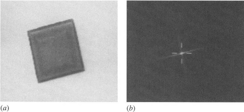
When applied to an object such as a square whose boundary consists of straight edges, the parametrization scheme outlined in the preceding section takes the following form: construct a transform in parameter space by moving inward from every boundary pixel by a distance equal to half the side S of the square and accumulate a line of votes of length S at each location, parallel to the local edge orientation. Then the pixel having the highest accumulation of votes is the center of the square. This technique was used to produce Fig. 14.1.

Figure 14.1 (a) Original off-camera gray-scale image of a square; (b) derived transform.

The GHT can be used in this way to detect all types of regular polygons, since in all such cases the center of the object can be chosen as the localization point L. Thus, to determine the positions at which lines of votes will be accumulated in parameter space, it is necessary merely to specify a displacement by the same distance along each edge normal. Taking a narrow rectangle as the lowest-order regular polygon (i.e., having two sides) and the circle as the highest-order polygon with an infinite number of short sides, it is apparent from Fig. 14.2 how the transform changes with the number of sides.

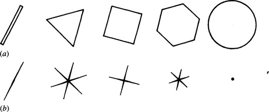
Figure 14.2 (a) Set of polygons; (b) associated transforms. The widths of the lines in (b) represent transform strength: ideally, the transform lines would have zero width.

In this scheme, notice that votes can be accumulated in parameter space using locally available edge orientation information and that the method is not muddled by changes in object orientation. This is true only for regular polygons, where the sides are equidistant from the localization point L. For more general shapes, including the quadrilateral in Fig. 14.3, the standard method of applying the GHT is to have a set of voting planes in parameter space, each corresponding to a possible orientation of the object. To find general shapes and orient them within 1°, 360 parameter planes appear to be required. This would incur a serious storage and search problem. Next we show how this problem may be minimized in the case of irregular polygons.

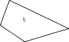
Figure 14.3 Geometry of a typical irregular polygon: the localization point L is at different distances from each of the sides of the polygon.

14.3.1 The Case of an Arbitrary Triangle

The case of an arbitrary triangle can be tackled by making use of the well-known property of the triangle that it possesses a unique inscribed circle. Thus, a localization point can be defined which is equidistant from the three sides. This means that the transform of any triangle can be found by moving into the triangle a specified distance from any side and accumulating the results in a single parameter plane (see Fig. 14.4). Such a parametrization can cope with random orientations of a triangle of given size and shape. However, this result is not wholly optimal because the separate transforms for each of the three sides do not peak at exactly the same point (except for an equilateral triangle). Neither should the lengths of the edge pixel transforms be the same. Each of these factors results in some loss of sensitivity. Thus, this solution optimizes the situation for storage and search speed but violates the condition for optimal sensitivity. If desired, this tradeoff could be reversed by reverting to the use of a large number of storage planes in parameter space, as described in Section 14.3. A better approach will be described in Section 14.3.3. Finally, note that the method is applicable only to a very restricted class of irregular polygons.

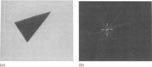
Figure 14.4 (a) Off-camera image of a triangle; (b) transform in a single parameter plane, making use of a localization point L which is equidistant from the three sides. An optimized transform requires four parameter planes (see Fig. 14.7).

14.3.2 The Case of an Arbitrary Rectangle

The case of a rectangle is characterized by greater symmetry than that for an arbitrary quadrilateral. In this case the number of parameter planes required to cope with variations in orientation may be reduced from a large number (e.g., 360—see Section 14.3) to just two. This is achieved in the following way. Suppose first that the major axis of the rectangle (of sides A, B: A>B)is known to be oriented between 0° and 90°. Then we need to accumulate votes by moving a distance B/2 from edge pixels oriented between 0° and 90° and accumulating a line of votes of length A in parameter space, and by moving a distance A/2 from edge pixels oriented between 90° and 180° and accumulating a line of votes of length B in parameter space. This is very similar to the situation for a square (see Section 14.3). However, suppose that the major axis was instead known to be oriented between 90^° and 180^°. Then we would need to change the method of transform suitably by interchanging the values of A and B. Since we do not know which supposition is true, we have to try both methods of transform, and for this purpose we need two planes in parameter space. If a strong peak is obtained in the first plane, the first supposition is true and the rectangle major axis is oriented between 0^° and 90^°—and vice versa if the strong peak is in the second plane in parameter space. In either case, the position of the strong peak indicates the position of the center of the rectangle (see Fig. 14.5).

Figure 14.5 (a) Off-camera image of a rectangle; (b), (c) optimized transforms in two parameter planes. The first plane (b) contains the highest peak, thereby indicating the position of the rectangle and its orientation within 90 °.

In summary, the largest peak in either plane indicates (1) which assumption about the orientation of the rectangle was justified and (2) the precise location of the rectangle. Apart from its inherent value, this example is important in giving a clue about how to develop the parametrization as symmetry is gradually reduced.

14.3.3 Lower Bounds on the Numbers of Parameter Planes

This section generalizes the solution of the previous section. First, note that two planes in parameter space are needed for optimal rectangle detection and that each of these planes may be taken to correspond to a range of orientations of the major axis.

For arbitrarily oriented polygons of known size and shape, votes must be accumulated in a number of planes in parameter space. Suppose that the polygon has N sides and that we are using M parameter planes to locate it. Since the complete range of possible orientations of the object is 2π, each of the M planes will have to be taken to represent a range 2π/M of object orientations. On detecting an edge pixel in the image, its orientation does not make clear which of the N sides of the object it originated from, and it is necessary to insert a line of votes at appropriate positions in N of the parameter planes. When every edge pixel has been processed in this way, the plane with the highest peak again indicates both the location of the object and its approximate orientation. Already it is clear that we must ensure that M>N, or else false peaks will start to appear in at least one of the planes, implying some ambiguity in the location of the object. Having obtained some feel for the problem, we now study the situation in more detail in order to determine the precise restriction on the number of planes.

Take {φ: i = 1,…, N} as the set of angles of the edge normals of the polygon in a standard orientation a. Next, suppose an edge of edge normal orientation 6 is found in the image. If this is taken to arise from side i of the polygon, we are assuming that the polygon has orientation α+θ—φ_i, and we accumulate a line of votes in parameter plane K_i = (α+θ—φ_i)(/(2π/M). (Here we force an integer result in the range 0 to M—1.) It is necessary to accumulate N lines of votes in the set of N parameter planes {K_i: i = 1,…, N}, as stated above. However, additional false peaks will start to appear in parameter space if an edge point on any one side of the polygon gives rise to more than one line of votes in the same parameter plane. To ensure that this does not occur it is necessary to ensure that K_i ≠ Kj for different i, j. Thus, we must have

     (14.1)

This result has the simple interpretation that the minimum exterior angle of the polygon ψ_min must be greater than 2π/M, the exterior angle being (by definition) the angle through which one side of the polygon has to be rotated before it coincides with an adjacent side (Fig. 14.6). Thus, the minimum exterior angle describes the maximum amount of rotation before an unnecessary ambiguity is generated about the orientation of the object. If no unnecessary ambiguity is to occur, the number of planes M must obey the condition

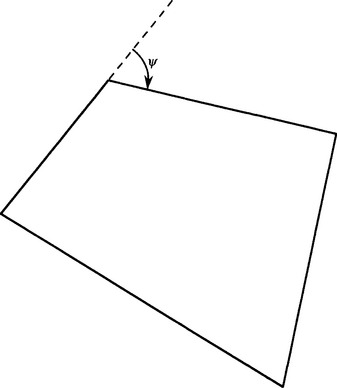
Figure 14.6 The exterior angle of a polygon, ψ angle through which one side has to be rotated before it coincides with an adjacent side.

     (14.2)

We are now in a position to reassess all the results so far obtained with polygon detection schemes. Consider regular polygons first: if there are N sides, then the common exterior angle is ψ= 2π/N, so the number of planes required is inherently

     (14.3)

However, symmetry dictates that all N planes contain the same information, so only one plane is required.

Consider next the rectangle case. Here the exterior angle is π/2, and the inherent number of planes is four. However, symmetry again plays a part, and just two planes are sufficient to contain all the relevant information, as has already been demonstrated.

In the triangle case, for a nonequilateral triangle the minimum exterior angle is typically greater than π/2 but is never as large as 2π/3. Hence, at least four planes are needed to locate a general triangle in an arbitrary orientation (see Fig. 14.7). Note, however, that for a special choice of localization point fewer planes are required—as shown in Section 14.3.1.

Figure 14.7 An arbitrary triangle and its transform in four planes: (a) localization point L selected to optimize sensitivity; (b)–(e) four planes required in parameter space.

Next, for a polygon that is almost regular, the minimum exterior angle is just greater than 2π/N, so the number of planes required is N + 1. In this case, it is at first surprising that as symmetry increases, the requirement jumps from N +1 planes, not to N planes but straight to one plane.

Now consider a case where there is significant symmetry but the polygon cannot be considered to be fully regular. Figure 14.8a exhibits a semiregular hexagon for which the set of identity rotations forms a group of order 3. Here the minimum exterior angle is the same as for a regular hexagon. Thus, the basic rule predicts that we need a total of six planes in parameter space. However, symmetry shows that only two of these contain different information. Generalizing this result, we find that the number of planes actually required is N/G rather than N, G being the order of the group of identity rotations of the object. To prove this more general result, note that we need to consider only object orientations in the range 0 to 2π/G instead of 0 to 2tt. Hence, condition (14.2) now becomes

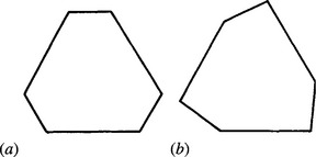
Figure 14.8 (a) Semiregular hexagon with threefold rotation symmetry and having all its exterior angles equal: two planes are required in parameter space in this case; (b) a similar hexagon with two slightly different exterior angles. Here three planes are needed in parameter space.

     (14.4)

Suppose instead that the hexagon had threefold rotation symmetry but had two sets of exterior angles with slightly different values (see Fig. 14.8b). Then

     (14.5)

and at best we will have M = (N/G) +1, which is 3 for the hexagon shape of Fig. 14.8b.

14.4 Determining Polygon Orientation

Having located a given polygon, it is usually necessary to determine its orientation. One way of proceeding is to find first all the edge points that contribute to a given peak in parameter space and to construct a histogram of their edge orientations. The orientation η of the polygon can be found if the positions of the peaks in this histogram are now determined and matched against the set {φ_i: i = 1,…, N} of the angles of the edge normals for the idealized polygon in standard orientation α (Section 14.3.3).

This method is wasteful in computation, however, since it does not make use of the fact that the main peak in parameter space has been found to lie in a particular plane K. Hence, we can take the set of (averaged) polygon side orientations θ from the histogram already constructed, identify which sides had which orientations, deduce from each θ a value for the polygon orientation η =α +θ—φ_i (see Section 14.3.3), and enter this value into a histogram of estimated t) values. The peak in this histogram will eventually give an accurate value for the polygon orientation).

Strong similarities, but also significant differences, are evident between the procedure described above and that described in Chapter 13 for the determination of ellipse parameters. In particular, both procedures are two-stage ones, in which it is computationally more efficient to find object location before object orientation.

14.5 Why Corner Detection?

Our analysis has shown the possibilities for direct detection of polygons, but it has also revealed the limitations of the approach: these arise specifically with more complex polygons—such as those having concavities or many sides. In such cases, it may be easier to revert to using line or corner detection schemes coupled with the abstract pattern matching approaches discussed in Chapter 15.

In previous chapters we noted that objects are generally located most efficiently from their features. Prominent features have been seen to include straight lines, arcs, holes, and corners. Corners are particularly important since they may be used to orient objects and to provide measures of their dimensions—a knowledge of orientation being vital on some occasions, for example if a robot is to find the best way of picking up the object, and measurement being necessary in most inspection applications. Thus, accurate, efficient corner detectors are of great relevance in machine vision. In the remainder of the chapter we shall focus on corner detection procedures.

Workers in this field have devoted considerable ingenuity to devising corner detectors, sometimes with surprising results (see, for example, the median-based detector described later in this chapter). We start by considering what is perhaps the most obvious detection scheme—that of template matching.

14.6 Template Matching

Following our experience with template matching methods for edge detection (Chapter 5), it would appear to be straightforward to devise suitable templates for corner detection. These would have the general appearance of corners, and in a 3 × 3 neighborhood they would take forms such as the following:

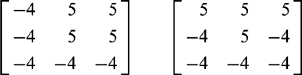
the complete set of eight templates being generated by successive 90^° rotations of the first two shown. Bretschi (1981) proposed an alternative set of templates. As for edge detection templates, the mask coefficients are made to sum to zero so that corner detection is insensitive to absolute changes in light intensity. Ideally, this set of templates should be able to locate all corners and to estimate their orientation to within 22.5^°.

Unfortunately, corners vary considerably in a number of their characteristics, including in particular their degree of pointedness,¹ internal angle, and the intensity gradient at the boundary. Hence, it is quite difficult to design optimal corner detectors. In addition, generally corners are insufficiently pointed for good results to be obtained with the 3 x 3 template masks shown above. Another problem is that in larger neighborhoods, not only do the masks become larger but also more of them are needed to obtain optimal corner responses, and it rapidly becomes clear that the template matching approach is likely to involve excessive computation for practical corner detection. The alternative is to approach the problem analytically, somehow deducing the ideal response for a corner at any arbitrary orientation, and thereby bypass the problem of calculating many individual responses to find which one gives the maximum signal. The methods described in the remainder of this chapter embody this alternative philosophy.

14.7 Second-order Derivative Schemes

Second-order differential operator approaches have been used widely for corner detection and mimic the first-order operators used for edge detection. Indeed, the relationship lies deeper than this. By definition, corners in gray-scale images occur in regions of rapidly changing intensity levels. By this token, they are detected by the same operators that detect edges in images. However, corner pixels are much rarer² than edge pixels. By one definition, they arise where two relatively straight-edged fragments intersect. Thus, it is useful to have operators that detect corners directly, that is, without unnecessarily locating edges. To achieve this sort of discriminability, it is necessary to consider local variations in image intensity up to at least second order. Hence, the local intensity variation is expanded as follows:

     (14.6)

where the suffices indicate partial differentiation with respect to x and y and the expansion is performed about the origin X₀ (0, 0). The symmetrical matrix of second derivatives is:

     (14.7)

This gives information on the local curvature at X₀. A suitable rotation of the coordinate system transforms 1(₂) into diagonal form:

     (14.8)

where appropriate derivatives have been reinterpreted as principal curvatures at X0.

We are particularly interested in rotationally invariant operators, and it is significant that the trace and determinant of a matrix such as 1(₂) are invariant under rotation. Thus we obtain the Beaudet (1978) operators:

     (14.9)

and

     (14.10)

It is well known that the Laplacian operator gives significant responses along lines and edges and hence is not particularly suitable as a corner detector. On the other hand, Beaudet’s “DET” (determinant) operator does not respond to lines and edges but gives significant signals near corners. It should therefore form a useful corner detector. However, DET responds with one sign on one side of a corner and with the opposite sign on the other side of the corner. At the point of real interest—on the corner—it gives a null response. Hence, rather more complicated analysis is required to deduce the presence and exact position of each corner (Dreschler and Nagel, 1981; Nagel, 1983). The problem is clarified by Fig. 14.9. Here the dotted line shows the path of maximum horizontal curvature for various intensity values up the slope. The DET operator gives maximum response at positions P and Q on this line, and the parts of the line between P and Q must be explored to find the “ideal” corner point C where DET is zero.

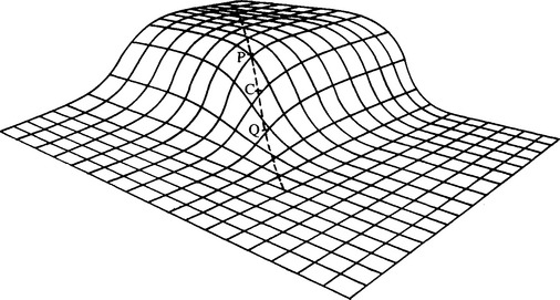
Figure 14.9 Sketch of an idealized corner, taken to give a smoothly varying intensity function. The dotted line shows the path of maximum horizontal curvature for various intensity values up the slope. The DET operator gives maximum responses at P and Q, and it is required to find the ideal corner position C where DET gives a null response.

Perhaps to avoid rather complicated procedures of this sort, Kitchen and Rosenfeld (1982) examined a variety of strategies for locating corners, starting from the consideration of local variation in the directions of edges. They found a highly effective operator that estimates the projection of the local rate of change of gradient direction vector along the horizontal edge tangent direction, and showed that it is mathematically identical to calculating the horizontal curvature k of the intensity function I. To obtain a realistic indication of the strength of a corner, they multiplied k by the magnitude of the local intensity gradient g:

     (14.11)

Finally, they used the heuristic of nonmaximum suppression along the edge normal direction to localize the corner positions further.

In 1983, Nagel was able to show that mathematically the Kitchen and Rosenfeld (KR) corner detector using nonmaximum suppression is virtually identical to the Dreschler and Nagel (DN) corner detector. A year later, Shah and Jain (1984) studied the Zuniga and Haralick (ZH) corner detector (1983) based on a bicubic polynomial model of the intensity function. They showed that this is essentially equivalent to the KR corner detector. However, the ZH corner detector operates rather differently in that it thresholds the intensity gradient and then works with the subset of edge points in the image, only at that stage applying the curvature function as a corner strength criterion. By making edge detection explicit in the operator, the ZH detector eliminates a number of false corners that would otherwise be induced by noise.

The inherent near-equivalence of these three corner detectors need not be overly surprising, since in the end the different methods would be expected to reflect the same underlying physical phenomena (Davies, 1988d). However, it is gratifying that the ultimate result of these rather mathematical formulations is interpretable by something as easy to visualize as horizontal curvature multiplied by intensity gradient.

14.8 A Median-Filter-Based Corner Detector

Paler et al. (1984) devised an entirely different strategy for detecting corners. This strategy adopts an initially surprising and rather nonmathematical approach based on the properties of the median filter. The technique involves applying a median filter to the input image and then forming another image that is the difference between the input and the filtered images. This difference image contains a set of signals that are interpreted as local measures of corner strength.

Applying such a technique seems risky since its origins suggest that, far from giving a correct indication of corners, it may instead unearth all the noise in the original image and present this as a set of “corner” signals. Fortunately, analysis shows that these worries may not be too serious. First, in the absence of noise, strong signals are not expected in areas of background. Nor are they expected near straight edges, since median filters do not shift or modify such edges significantly (see Chapter 3). However, if a window is moved gradually from a background region until its central pixel is just over a convex object corner, there is no change in the output of the median filter. Hence there is a strong difference signal indicating a corner.

Paler et al. (1984) analyzed the operator in some depth and concluded that the signal strength obtained from it is proportional to (1) the local contrast and (2) the “sharpness” of the corner. The definition of sharpness they used was that of Wang et al. (1983), meaning the angle t through which the boundary turns. Since it is assumed here that the boundary turns through a significant angle (perhaps the whole angle t) within the filter neighborhood, the difference from the second-order intensity variation approach is a major one. Indeed, it is an implicit assumption in the latter approach that first- and second-order coefficients describe the local intensity characteristics with reasonable rigor, the intensity function being inherently continuous and differentiable. Thus, the second-order methods may give unpredictable results with pointed corners where directions change within the range of a few pixels. Although there is some truth in this, it is worth looking at the similarities between the two approaches to corner detection before considering the differences.

14.8.1 Analyzing the Operation of the Median Detector

This subsection considers the performance of the median corner detector under conditions where the gray-scale intensity varies by only a small amount within the median filter neighborhood region. This permits the performance of the corner detector to be related to low-order derivatives of the intensity variation, so that comparisons can be made with the second-order corner detectors mentioned earlier.

To proceed, we assume a continuous analog image and a median filter operating in an idealized circular neighborhood. For simplicity, since we are attempting to relate signal strengths and differential coefficients, we ignore noise. Next, recall (Chapter 3) that for an intensity function that increases monotonically with distance in some arbitrary direction x but that does not vary in the perpendicular direction y, the median within the circular window is equal to the value at the center of the neighborhood. Thus, the median corner detector gives zero signal if the horizontal curvature is locally zero.

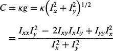
If there is a small horizontal curvature k, the situation can be modeled by envisaging a set of constant-intensity contours of roughly circular shape and approximately equal curvature within the circular window that will be taken to have radius a (Fig. 14.10). Consider the contour having the median intensity value. The center of this contour does not pass through the center of the window but is displaced to one side along the negative x-axis. Furthermore, the signal obtained from the corner detector depends on this displacement. If the displacement is D, it is easy to see that the corner signal is Dg₂ since g₂ allows the intensity change over the distance D to be estimated (Fig. 14.10). The remaining problem is to relate D to the horizontal curvature k. A formula giving this relation has already been obtained in Chapter 3. The required result is:

Figure 14.10 (a) Contours of constant intensity within a small neighborhood. Ideally, these are parallel, circular, and of approximately equal curvature (the contour of median intensity does not pass through the center of the neighborhood); (b) cross section of intensity variation, indicating how the displacement D of the median contour leads to an estimate of corner strength.

     (14.12)

so the corner signal is

     (14.13)

Note that C has the dimensions of intensity (contrast) and that the equation may be reexpressed in the form:

     (14.14)

so that, as in the formulation of Paler et al. (1984), corner strength is closely related to corner contrast and corner sharpness.

To summarize, the signal from the median-based corner detector is proportional to horizontal curvature and to intensity gradient. Thus, this corner detector gives an identical response to the three second-order intensity variation detectors discussed in Section 14.7, the closest practically being the KR detector. However, this comparison is valid only when second-order variations in intensity give a complete description of the situation. The situation might be significantly different where corners are so pointed that they turn through a large proportion of their total angle within the median neighborhood. In addition, the effects of noise might be expected to be rather different in the two cases, as the median filter is particularly good at suppressing impulse noise. Meanwhile, for small horizontal curvatures, there ought to be no difference in the positions at which median and second-order derivative methods locate corners, and accuracy of localization should be identical in the two cases.

14.8.2 Practical Results

Experimental tests with the median approach to corner detection have shown that it is a highly effective procedure (Paler et al., 1984; Davies, 1988d). Corners are detected reliably, and signal strength is indeed roughly proportional both to local image contrast and to corner sharpness (see Fig. 14.11). Noise is more apparent for 3 × 3 implementations, which makes it better to use 5 × 5 or larger neighborhoods to give good corner discrimination. However, because median operations are slow in large neighborhoods and background noise is still evident even in 5 × 5 neighborhoods, the basic median-based approach gives poor performance by comparison with the second-order methods. However, both of these disadvantages are virtually eliminated by using a “skimming” procedure in which edge points are first located by thresholding the edge gradient, and the edge points are then examined with the median detector to locate the corner points (Davies, 1988d). With this improved method, performance is found to be generally superior to that for, say, the KR method in that corner signals are better localized and accuracy is enhanced. Indeed, the second-order methods appear to give rather fuzzy and blurred signals that contrast with the sharp signals obtained with the improved median approach (Fig. 14.12).

Figure 14.11 (a) Original off-camera 128 × 128 6-bit gray-scale image; (b) result of applying the median-based corner detector in a 5 × 5 neighborhood. Note that corner signal strength is roughly proportional both to corner contrast and to corner sharpness.

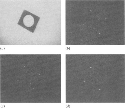
Figure 14.12 Comparison of the median and KR corner detectors: (a) original 128 × 128 gray-scale image; (b) result of applying a median detector; (c) result of including a suitable gradient threshold; (d) result of applying a KR detector. The considerable amount of background noise is saturated out in (a) but is evident from (b). To give a fair comparison between the median and KR detectors, 5 × 5 neighborhoods are employed in each case, and nonmaximum suppression operations are not applied. The same gradient threshold is used in (c) and (d).

At this stage the reason for the more blurred corner signals obtained using the second-order operators is not clear. Basically, there is no valid rationale for applying second-order operators to pointed corners, since higher derivatives of the intensity function will become important and will at least in principle interfere with their operation. However, it is evident that the second-order methods will probably give strong corner signals when the tip of a pointed corner appears anywhere in their neighborhood, so there is likely to be a minimum blur region of radius a for any corner signal. This appears to explain the observed results adequately. The sharpness of signals obtained by the KR method may be improved by nonmaximum suppression (Kitchen and Rosenfeld, 1982; Nagel, 1983). However, this technique can also be applied to the output of median-based corner detectors. Hence, the fact remains that the median-based method gives inherently better localized signals than the second-order methods (although for low-curvature corners the signals have similar localization).

Overall, the inherent deficiencies of the median-based corner detector can be overcome by incorporating a skimming procedure, and then the method becomes superior to the second-order approaches in giving better localization of corner signals. The underlying reason for the difference in localization properties appears to be that the median-based signal is ultimately sensitive only to the particular few pixels whose intensities fall near the median contour within the window, whereas the second-order operators use typical convolution masks that are in general sensitive to the intensity values of all the pixels within the window. Thus, the KR operator tends to give a strong signal when the tip of a pointed corner is present anywhere in the window.

14.9 The Hough Transform Approach to Corner Detection

In certain applications, corners might rarely appear in the idealized pointed form suggested earlier. Indeed, in food applications corners are commonly chipped, crumbly, or rounded, and are bounded by sides that are by no means straight lines (Fig. 14.13). Even mechanical components may suffer chipping or breakage. Hence, it is useful to have some means of detecting these types of nonideal corners. The generalized HT provides a suitable technique (Davies, 1986b, 1988a).

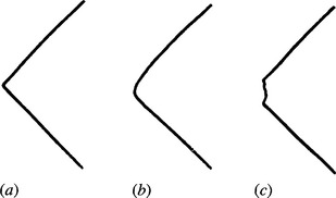
Figure 14.13 Types of corners: (a) pointed; (b) rounded; (c) chipped. Corners of type (a) are normal with metal components, those of type (b) are usual with biscuits and other food products, whereas those of type (c) are common with food products but rarer with metal parts.

The method used is a variation on that described in Section 14.3 for locating objects such as squares. Instead of accumulating a line of candidate center points parellel to each side after moving laterally inward a distance equal to half the length of a side, only a small lateral displacement is required when locating corners. The lateral displacement that is chosen must be sufficient to offset any corner bluntness, so that the points that are located by the transform lines are consistently positioned relative to the idealized corner point (Fig. 14.14). In addition, the displacement must be sufficiently large that enough points on the sides of the object contribute to the corner transforms to ensure adequate sensitivity.

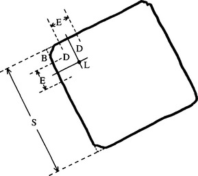
Figure 14.14 Geometry for locating blunt corners: B, region of bluntness; D, lateral displacement employed in edge pixel transform; E, distance over which position of corner is estimated; I, idealized corner point; L, localization point of a typical corner; S, length of a typical side. The degree of corner bluntness shown here is common among food products such as fishcakes.

There are two relevant parameters for the transform: D, the lateral displacement, and T, the length of the transform line arising from each edge point. These parameters must be related to the following parameters for the object being detected: B, the width ofthe corner bluntness region (Fig. 14.14), and S, the length of the object side (for convenience the object is assumed to be a square). E, the portion of a side that is to contribute to a corner peak, is simply related to T:

     (14.15)

Since we wish to make corner peaks appear as close to idealized corners as possible, we may also write:

     (14.16)

These definitions now allow the sensitivity of corner location to be optimized. Note first that the error in the measurement of each corner position is proportional to since our measurement of the relevant part of each side is effectively being averaged over E independent signals. Next, note that the purpose of locating corners is ultimately to measure (1) the orientation of the object and (2) its linear dimensions. Hence, the fractional accuracy is proportional to:

     (14.17)

Eliminating D now gives:

     (14.18)

Differentiating, we find:

     (14.19)

Accuracy can now be optimized by setting dA/dE =0, so that:

     (14.20)

making

     (14.21)

Hence, there is a clear optimum in accuracy, and as B →0 it occurs for D S/6, whereas for rather blunt or crumbly types of objects (typified by biscuits) B S/8 and then D S/4.

If optimal object detection and location had been the main aim, this would have been achieved by setting E = S—2B and detecting all the corners together at the center of the square. It is also possible that by optimizing object orientation, object detection is carried out with reduced sensitivity, since only a length 2E of the perimeter contributes to each signal, instead of a length 4S— 8B.

The calculations presented here are important for a number of reasons: (1) they clarify the point that tasks such as corner location are carried out not in isolation but as parts of larger tasks that are optimizable; (2) they show that the ultimate purpose of corner detection may be either to locate objects accurately or to orient and measure them accurately; and (3) they indicate that there is an optimum region of interest E for any operator that is to locate corners. This last factor has relevance when selecting the optimum size of neighborhood for the other corner detectors described in this chapter.

Although the calculations above emphasized sensitivity and optimization, the underlying principle of the HT method is to find corners by interpolation rather than by extrapolation, as interpolation is generally a more accurate procedure. The fact that the corners are located away from the idealized corner positions is to some extent a disadvantage (although it is difficult to see how a corner can be located directly if it is missing). However, once the corner peaks have been found, for known objects the idealized corner positions may be deduced (Fig. 14.15). It is as well to note that this step is unlikely to be necessary if the real purpose of corner location is to orient the object and to measure its dimensions.

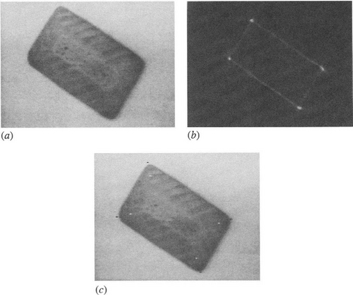
Figure 14.15 Example of the Hough transform approach: (a) original image of a biscuit (128 × 128 pixels, 64 gray levels); (b) transform with lateral displacement around 22% of the shorter side; (c) image with transform peaks located (white dots) and idealized corner positions deduced (black dots). The lateral displacement employed here is close to the optimum for this type of object.

14.10 The Plessey Corner Detector

At this point we consider whether other strategies for corner detection could be devised. The second-order derivative class of corner detector was devised on the basis that corners are ideal, smoothly varying differentiable intensity profiles, whereas the median-based detector was conceived totally independently on the basis of curved step edges whose profiles are quite likely not to be smoothly varying and differentiable. It is profitable to take the latter idea further and to consider corners as the intersection of two step edges.

First, imagine that a small region, which is the support region of such a corner detector, contains both a step edge aligned along the x direction and another aligned along the y direction. To detect these edges, we can use an operator that estimates <I_x> and another that estimates <I_y>. Note that a corner detector would have to detect both types of edges simultaneously. To do so, we can use a combined estimator such as <|I_x><|I_y|> or <I_x²><I_y²>. Each of these operators leads to corner signals that can be thresholded conveniently using a single positive threshold value.

Next, note that this estimator requires the edge orientations to be known and indeed aligned along the x-andy-axes directions. To obtain more general properties, the operator needs to transform appropriately under rotation of axes. In addition, magnitudes are difficult to handle mathematically, so we start with the squared magnitude estimator and employ a symmetrical matrix of first derivatives in the transformable form:

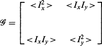     (14.22)

where

     (14.23)

This expression would clearly be identically zero if evaluated separately at each individual pixel. Nevertheless, our intuition is correct, and the base parameters < I_x² >, < I_y² >, and < I_xI_y > must all be determined as averages over all pixels in the detector support region. If this is done, the expression need not average to zero, as the interpixel variations leading to the three base parameter values will introduce deviations. This situation is easily demonstrated, as rotation of axes to permit diagonalization of the matrix yields:

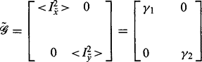     (14.24)

with eigenvalues < I_x²_~ > = Y₁, < I_y²_~ > = Y₂. In this case, the Hessian is Y₁Y₂,and this is a sensible value to take for the corner strength. In particular, it is substantial only if both edges are present within the support region. The Plessey operator (Harris and Stephens, 1988; see also Noble, 1988) normalizes this measure by dividing by y ₁ + y₂ and forming a square root:³

     (14.25)

Interestingly, this does not ruin the transformation properties of the operator because both the determinant and the trace of the relevant symmetrical matrix are invariant under orthogonal transformations.

This operator has some useful properties. In particular, it is better to call it an “interest” operator rather than a corner detector because it also responds to situations where the two constituent edges cross over, so that a double corner results (as happens in many places on a checkerboard). It is really responding to and averaging the effects of all the locations where two edges appear within the operator support region. We can easily show that it has this property, as the fact that the operator embodies < I²_x > and < I? > means that it is insensitive to the sign of the local edge gradients (Fig. 14.16a).

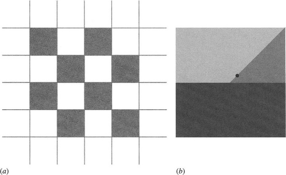
Figure 14.16 Effect of the Plessey corner detector. (a) shows a checkerboard pattern that gives high responses at each of the edge crossover points. Because of symmetry, the location of the peaks is exactly at the crossover locations. (b) Example of a T-junction. The black dot shows a typical peak location. In this case there is no symmetry to dictate that the peak must occur exactly at the T-junction.

The Plessey operator also has the undesirable property⁴ that it can give a bias at T-junctions, to an extent dependent on the relative intensities of the three adjacent regions (Fig. 14.16b). This is the effect of averaging the three base parameters over the whole support region. It is difficult to be absolutely sure where the peak response will be as the computation is quite complex. In such cases, symmetry can act as a useful constraining factor—as in the case of a double corner on a checkerboard, where the peak signal necessarily coincides with the double corner location. (This applies to all the edge crossover points in Fig. 14.16a.) Clearly, noise will have some effect on the peak locations in off-camera images.

14.11 Corner Orientation

This chapter has so far considered the problem of corner detection as relating merely to corner location. However, corners differ from holes in that they are not isotropic, and hence they are able to provide orientation information. Such information can be used by procedures that collate the information from various features in order to deduce the presence and positions of objects containing them. In Chapter 15 we will see that orientation information is valuable in immediately eliminating a large number of possible interpretations of an image, and hence of quickly narrowing down the search problem and saving computation.

Clearly, when corners are not particularly pointed, or are detected within rather small neighborhoods, the accuracy of orientation will be somewhat restricted. However, orientation errors will seldom be worse than 90° and will often be less than 20°. Although these accuracies are far worse than those (around 1 ^°) for edge orientation (see Chapter 5), they provide valuable constraints on possible interpretations of an image.

Here we consider only simple means of estimating corner orientation. Basically, once a corner has been located accurately, it is a rather trivial matter to estimate the orientation of the intensity gradient at that location. The main problem that arises is that a slight error in locating the corner gives a bias in estimating its orientation toward that of one or another of the bounding sides—and for a sharp pointed corner, this can mean an error approaching 90°. The simplest solution to this problem is to find the mean orientation over a small region surrounding the estimated corner position. Then, without excessive computation, the orientation accuracy will usually be within the 20° limit suggested above.

14.12 Concluding Remarks

When using the GHT for the detection of polygons, it is useful to try to minimize storage and computation. In some cases only one parameter plane is needed to detect a polygonal object: commonly, a number of parameter planes of the order of the number of sides of the polygon is required, but this still represents a significant saving compared with the numbers needed to detect general shapes. It has been demonstrated how optimal savings can be achieved by taking into account the symmetry possessed by many polygon shapes such as squares and rectangles.

The analysis has shown the possibilities for direct detection of polygons, but it has also revealed the limitations of this approach. These limitations arise specifically with more complex polygons—such as those having concavities or many sides. In such cases, it may be easier to revert to using line or corner detection schemes coupled with the abstract pattern matching approaches discussed in Chapter 15. Indeed, the latter approach offers the advantage of greater resistance to shape distortions if suitable algorithms to infer the presence of objects can be found.

Hence, the chapter also appropriately examined corner detection schemes. Apart from the obvious template matching procedure, which is strictly limited in its application, and its derivative, the lateral histogram method (see Problems 14.5 and 14.6), three main approaches have been described. The first was the second-order derivative approach, which includes the KR, DN, and ZH methods—all of which embody the same basic schema. The second was the median-based method, which turned out to be equivalent to the second-order methods—but only in situations where corners have smoothly varying intensity functions; the third was a Hough-based scheme that is particularly useful when corners are liable to be blunt, chipped, or damaged. The analysis of this last scheme revealed interesting general points about the specification and design of corner detection algorithms.

Although the median-based approach has obvious inherent disadvantages—its slowness and susceptibility to noise—these negative aspects can largely be overcome by a skimming (two-stage template matching) procedure. Then the method becomes essentially equivalent to the second-order derivative methods for low-curvature intensity functions, as stated above. However, for pointed corners, higher-order derivatives of the intensity function are bound to be important. As a result the second-order methods are based on an unjustifiable rationale and are found to blur corner signals, hence reducing the accuracy of corner localization. This problem does not arise for the median-based method, which seems to offer rather superior performance in practical situations. Clearly, however, it should not be used when image noise is excessive, as then the skimming procedure will either (with a high threshold) remove a proportion of the corners with the noise, or else (with a low threshold) not provide adequate speedup to counteract the computational load of the median filtering routine.

Overall, the Plessey corner detector described in Section 14.10 and more recently the SUSAN detector (Smith and Brady, 1997) have been among the most widely used of the available corner detectors, though whether this is the result of conclusive tests against carefully defined criteria is somewhat doubtful. For more details and comparisons, see the next section.

14.13 Bibliographical and Historical Notes

The initial sections of this chapter arose from the author’s own work which was aimed at finding optimally sensitive means of locating shapes, starting with spatial matched filters. Early work in this area included that of Sklansky (1978), Ballard (1981), Brown (1983), and Davies (1987c), which compared the HT approach with spatial matched filters. These general investigations led to more detailed studies of how straight edges are optimally detected (Davies, 1987d,j), and then to polygon detection (Davies, 1986d, 1989c). Although optimal sensitivity is not the only criterion for effectiveness of object detection, nonetheless it is of great importance, since it governs both effectiveness per se (especially in the presence of “clutter” and occlusion) and the accuracy with which objects may be located.

The emphasis on spatial matched filters seemed to lead inevitably to use of the GHT, with its accompanying computational problems. The present chapter should make it plain that although these problems are formidable, systematic analysis can make a significant impact on them.

Corner detection is a subject that has been developing for well over two decades. Beaudet’s (1978) work on rotationally invariant image operators set the scene for the development of parallel corner detection algorithms. This was soon followed by Dreschler and Nagel’s (1981) more sophisticated second-order corner detector. The motivation for their research was mapping the motion of cars in traffic scenes, with corners providing the key to unambiguous interpretation of image sequences. One year later, Kitchen and Rosenfeld (1982) had completed their study of corner detectors based mainly on edge orientation and had developed the second-order KR method described in Section 14.7. The years 1983 and 1984 saw the development of the lateral histogram corner detector, the second-order ZH detector, and the median-based detector (Wu and Rosenfeld, 1983; Zuniga and Haralick, 1983; Paler et al., 1984). Subsequently,

Davies’ work on the detection of blunt corners and on analyzing and improving the median-based detector appeared (1986b, 1988a,d, 1992a). These papers form the basis of Sections 14.8 and 14.9. Meanwhile, other methods had been developed, such as the Plessey algorithm (Harris and Stephens, 1988; see also Noble, 1988), which is covered in Section 14.10. The much later algorithm of Seeger and Seeger (1994) is also of interest because it appears to work well on real (outdoor) scenes in real time without requiring the adjustment of any parameters.

The Smith and Brady (1997) SUSAN algorithm marked a further turning point, needing no assumptions on the corner geometry, for it works by making simple comparisons of local gray levels. This is one of the most often cited of all corner detection algorithms. Rosin (1999) adopted the opposite approach of modeling corners in terms of subtended angle, orientation, contrast, bluntness, and boundary curvature with excellent results. However, parametric approaches such as this tend to be computation intensive. Note also that parametric models sometimes run into problems when the assumptions made in the model do not match the data of real images. It is only much later, when many workers have tested the available operators, that such deficiencies come to light. The late 1990s also saw the arrival of a new boundary-based corner detector with good detection and localization (Tsai et al., 1999). A development of the Plessey detector called a gradient direction detector (Zheng et al., 1999)—which was optimized for good localization—also has reduced complexity.

In the 2000s, further corner detectors have been developed. The Ando (2000) detector, similar in concept to the Tsai et al. (1999) detector, has been found to have good stability, localization, and resolution. Liidtke et al. (2002) designed a detector based on a mixture model of edge orientation. In addition to being effective in comparison with the Plessey and SUSAN operators, particularly at large opening angles, the method provides accurate angles and strengths for the corners. Olague and Hernandez (2002) worked on a unit step-edge function (USEF) concept, which is able to model complex corners well. This innovation resulted in adaptable detectors that are able to detect corners with subpixel accuracy. Shen and Wang (2002) described a Hough-transform-based detector; as this works in a 1-D parameter space, it is fast enough for real-time operation. A useful feature of the Shen and Wang paper is the comparison with, and hence between, the Wang and Brady detector, the Plessey detector, and the SUSAN detector. Several example images show that it is difficult to know exactly what one is looking for in a corner detector (i.e., corner detection is an ill-posed problem), and that even the well-known detectors sometimes inexplicably fail to find corners in some very obvious places. Golightly and Jones (2003) present a practical problem in outdoor country scenery. They discuss not only the incidence of false positives and false negatives but also the probability of correct association in corner matching (e.g., during motion).

Rocket (2003) presents a performance assessment of three corner detection algorithms—the Kitchen-Rosenfeld detector, the median-based detector, and the Plessey detector. The results are complex, with the three detectors all having very different characteristics. Rocket’s paper is valuable because it shows how to optimize the three methods (not least showing that a particular parameter k for the Plessey detector should be ~0.04) and also because it concentrates on careful research, with no “competition” from detectors invented by its author. Finally, Tissainayagam and Suter (2004) assess the performance of corner detectors, relating this study specifically to point feature (motion) tracking applications. It would appear that whatever the potential value of other reviews, this one has particular validity within its frame of reference. Interestingly, it finds that, in image sequence analysis, the Plessey detector is more robust to noise than the SUSAN detector. A possible explanation is that it “has a built-in smoothing function as part of its formulation.”

This review of the literature covers many old and recent developments on corner detection, but it is not the whole story. In many applications, it is not specific corner detectors that are needed but salient point detectors. As indicated in Chapter 13, salient point features can be small holes or corners. However, they may also be characteristic patterns of intensity. Recent literature has referred to such patterns as interest points. Often interest point detectors are essentially corner detectors, but this does not have to be the case. For example, the Plessey detector is sometimes called an interest detector—with good reason, as indicated in Section 14.10. Moravec (1977) was among the first to refer to interest points. He was followed, for example, by Schmid et al. (2000), and later by Sebe and Lew (2003) and Sebe et al. (2003), who revert to calling them salient points but with no apparent change of meaning (except that the points should also be visually interesting). Overall, it is probably safest to use the Haralick and Shapiro (1993) definition: a point being “interesting” if it is both distinctive and invariant—that is, it stands out and is invariant to geometric distortions such as might result from moderate changes in scale or viewpoint. (Note that Haralick and Shapiro also list other desirable properties—stability, uniqueness, and interpretability.) The invariance aspect is taken up by Kenney et al. (2003) who show how to remove from consideration ill-conditioned points in order to make matching more reliable.

The considerable ongoing interest in corner detection and interest point detection underlines the point, made in Section 14.5, that good point feature detectors are vital to efficient image interpretation, as will be seen in more detail in subsequent chapters.

14.14 Problems