
Trigonometric functions and waves
5.1 Introduction
Waves occur naturally in a number of situations: the movement of disturbed water, the passage of sound through the air, vibrations of a plucked string. If the movement of a particular particle is plotted against time, then we get the distinctive wave shape, called a sinusoid. The mathematical expression of a wave is found by using the trigonometric functions, sine and cosine. In Chapter 6 of the Background Mathematics Notes on the companion website for this book we looked at right angled triangles and defined the trigonometric ratios. The maximum angle in a right angled triangle is 90° so to find the trigonometric functions, sin(t), cos(t), and tan(t) where t can be extended over the real numbers, we need a new way of defining them. This we do by using a rotating rod. Usually the function will be used to relate, for instance, the height of the rod to time. Therefore, it does not always make sense to think of the input to the cosine and sine functions as being an angle. This problem is overcome by using a new measure for the angle called the radian, which easily relates the angle to the distance travelled by the tip of the rotating rod.
Waves may interfere with each other, as for instance on a plucked string, where the disturbance bounces off the ends producing a standing wave. Amplitude modulation of, for instance, radio waves, works by the superposition of a message on a higher signal frequency. These situations require an understanding of what happens when two, or more cosine or sine functions are added, subtracted, or multiplied and hence we also study trigonometric identities.
5.2 Trigonometric functions and radians
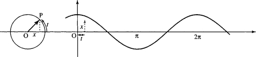
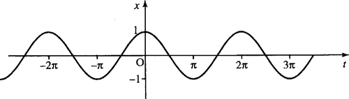
Consider a rotating rod of length 1. Imagine, for instance, that it is a position marked on a bicycle tyre at the tip of one of the spokes, as the bicycle travels along. The distance travelled by the tip of the rod in 1 complete revolution is 2π (the circumference of the circle of radius 1). The height of the rod (measured from the centre of the wheel), y, can be plotted against the distance travelled by the tip as in Figure 5.1.

Similarly, the position to the right or left of the origin, x, can be plotted against the distance travelled by the tip of the rod as in Figure 5.2. Figure 5.1 defines the function y = sin(t) and Figure 5.2 defines the function x = cos(t).
This definition of the trigonometric function is very similar to that used for the ratios in the triangle, if the hypotenuse is of length 1 unit. The definitions become the same for angles up to a right angle if radians are used as a measure of the angle in the triangle instead of degrees. Instead of 360° making a complete revolution 2π radians make a complete revolution. Some examples of degree to radian conversion are given in Figure 5.3.

To convert degrees to radians use the fact that 360° is the same as 2π radians or equivalently that 180° is the same as π radians. Hence, to convert degrees to radians multiply by π /180 and to convert radians to degrees multiply by 180/ π.
Remember that π is approximately 3.1416 so these conversions can be expressed approximately as: to convert degrees to radians multiply by 0.01745 (i.e. 1° ≈ 0.01745 radians) and to convert radians to degrees multiply by 57.3 (i.e. 1 radian ≈ 57.3°).
Example 5.1
(a) Express 45° in radians.
Multiply 45 by π/180 giving π/4 ≈ 0.785. Hence, 45° ≈ 0.785 radians.
(b) Express, 17° in radians.
Multiply 17 by π/180 giving 17π/180 ≈ 0.297. Hence 17° ≈ 0.297 radians.
(c) Express 120° in radians.
Multiply 120 by π/180 giving 2π/3 ≈ 2.094. Hence, 120° ≈ 2.094.
(d) Express 2 radians in degrees.
Multiply 2 by 180/π giving 114.6. Hence, 2 radians ≈114.6°.
(e) Express (5π/6) radians in degrees.
Multiply 5π/6 by 180/π giving 150. Hence, (5π/6) radians = 150°.
(f) Express 0.5 radians in degrees.
Multiply 0.5 by 180/π giving 28.6. Hence, 0.5 radians ≈28.6°.
The trigonometric functions can also be defined using a rotating rod of length r as in Figure 5.4.

The function values are given by:
![]()
Also
![]()
where α is measured in radians (one complete revolution is 2π radians).
Notice that the definitions are exactly the same as the trigonometric ratios, where r is the hypotenuse and x and y are the adjacent and opposite sides to the angle, except that x and y can now take both positive and negative values and the angles can be as big as we like or negative (if the rod rotates clockwise):


To get the correct function values from the calculator, it should be in ‘radian’ mode. However, by custom, engineers often use degrees, so we will use the convention that if the ‘units’ are not specified then radians must be used and for the input to be in degrees that must be expressly marked, for example cos(30°).
Important relationship between the sine and the cosine
From Pythagoras's theorem, looking at the diagram in Figure 5.4, we have x2 + y2 = r2. Dividing both sides by r2 we get:
![]()
![]()
and this is written in shorthand as
![]()
5.3 Graphs and important properties
We can now draw graphs of the functions for all input values t as in Figures 5.5–5.7.
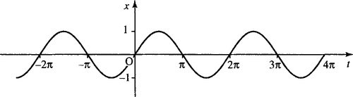

These are all important examples of periodic functions. To show that the cos(t) or sin(t) function is periodic, translate the graph to the left or right by 2π. The resulting graph will fit exactly on top of the original untranslated graph. 2π is called the fundamental period as translating by 4π, 6π, 8π, etc. also results in the graph fitting exactly on top of the original function. The fundamental period is defined as the smallest period that has this property and all other periods are multiples of the fundamental period. This periodic property can be expressed using a letter, n, to represent any integer, giving

That is, adding or subtracting any multiple of 2π from the value of t gives the same value of the functions x = cos(t) and y = sin(t).
The other important thing to remember about cos(t) and sin(t) is that although the domain of the functions is all the real numbers, the function values themselves lie between −1 and +1
![]()
We say that the functions are bounded by −1 and +1 or, in other words, the range of the cosine and sine functions is [−1, 1].
z = tan(t) has fundamental period π. If the graph is translated by π to the left or right, then the resulting graph will fit exactly on top of the original graph. This periodic property can be expressed using n to represent any integer, giving
![]()
The values of tan(t) are not bounded. We can also say that –∞ < tan(t) < ∞.
Symmetry
Other important properties of these functions are the symmetry of the functions. cos(t) is even, while sin(t) and tan(t) are odd. Unlike the terms odd and even when used to describe numbers, not all functions are either odd or even, most are neither. To show that cos(t) is even, reflect the graph along the vertical axis. The resulting graph is exactly the same as the original graph. This shows that swapping positive t values for negative ones has no difference on the function values, that is,
![]()
Other examples of even functions were given in Chapter 2 and the general property of even functions was given there as f(t) = f(–t). The functions sine and tangent are odd. If they are reflected along the vertical axis then the resulting graph is an upside down version of the original. This shows that swapping positive t values for negative ones gives the negative of the original function. This property can be expressed by

For a general function, y = f(t), the property of being odd can be expressed by f(–t) = −f(t).
The relationships between the sine and cosine
Take the graph of sin(t) and translate it to the left by 90° or π/2 and we get the graph of cos(t). Equivalently, take the graph of cos(t) and translate it to the right by π/2 and we get the graph of sin(t). Using the ideas of translating functions given in Chapter 2, we get

Other relationships can be shown using triangles as in Figure 5.8 giving

From Pythagoras theorem we also have that
![]()
dividing both sides by r2 we get

and using the definitions of sin(α) = a/r and cos(α) = b/r, we get
![]()
Rearranging this, we have cos2(α) = 1 – sin2(α) or sin2(α) = 1 – cos2(α).
Example 5.2
Given sin(A) = 0.5 and 0 ≤ A ≤ 90°, use trigonometric identities to find:
(b) sin(90° − A)
(c) cos(90° − A).
Solution
(a) Using cos2(A) = 1 – sin2(A) and sin(A) = 0.5
As A is between 0° and 90°, the cosine must be positive giving cos(A) ≈ 0.866.
(b) As sin(90° – A) = cos(A), sin(90° – A) ≈ 0.866.
(c) As cos(90° − A) = sin(A), cos(90° – A) = 0.5.
The functions A cos(at + b) + B and A sin(at + b) + B
The graph of these functions can be found by using the ideas of Chapter 2 for graph sketching.
Example 5.3
Sketch the graph of y against t, where
![]()
The stages in sketching this graph are shown in Figure 5.9.

Example 5.4
Sketch the graph of z against q where

The stages in sketches this graph are given in Figure 5.10.

 (a) start with z = sin(q); (b) shift to the right by π/4 to give z = sin(q – (π/4)); (c) squash the graph in the q-axis to give z = sin(πq – (π/4)); (d) squash the graph in the z-axis giving
  ; (e) translate in the z direction by
  to get
Amplitude, fundamental period, phase, and cycle rate
In Figure 5.11 are some examples of functions y = A cos(ax + b) and in each case the amplitude, phase, fundamental period, and cycle rate has been found. In Figure 5.11(a)
is drawn, and has a peak value of 0.5 and a trough value of −0.5. Therefore, the amplitude is half the difference: (0.5 – (–0.5)) /2 = 0.5. The period, or cycle length, is the minimum amount the graph needs to be shifted to the left or right (excluding no shift) in order to fit over the original graph. In this case the period is 0.4. The phase is found by finding the proportion of the cycle that the graph has been shifted to the left. In this case the proportion of shift is 1/4. Now multiply that by a standard cycle length of 2π to give the phase angle of π/2. The cycle rate is the number of cycles in unit length given by the reciprocal of the period = 1/0.4 = 2.5.
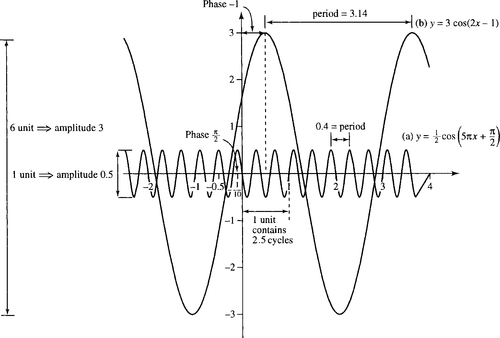
In Figure 5.11(b) y = 3 cos(2x − 1), has a peak value of 3 and a trough value of −3. Therefore, the amplitude is half the difference = (3 – (−3))/2 = 3. The period is the minimum amount the graph needs to be shifted to the left or right (excluding no shift) in order to fit over the original graph. In this case the period is π. The phase is found by finding the proportion of the cycle that the graph has been shifted to the left. In this case the proportion of shift is −0.5/π. Now multiply that by a standard cycle length of 2π to give the phase angle of −1. The cycle rate is the number of cycles in unit length given by the reciprocal of the period 1/π ≈ 0.32.
We can generalize from these examples to say that for the function y = A cos(ax + b), A positive, we have the following.
The amplitude is half the difference between the function values at the peak and the trough of the wave and in case where y = A cos(ax + b) is given by A.
The fundamental period, P, or cycle length is the smallest, non-zero, distance that the graph can be shifted to the right or left so that it lies on top of the original graph. This can be found by looking for two consecutive values where the function takes its maximum value, that is when the cosine takes the value 1. Using the fact that cos(0) = 1 and cos(2π) = 1,

and the difference between them is 2π/a; giving the fundamental period of the function cos(ax + b) as 2π/a.
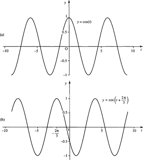
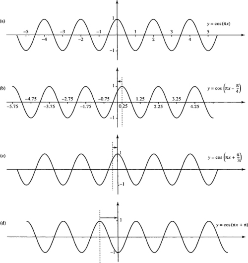
The phase is given by the number, b, in the expression A cos (ax + b). The phase is related to the amount the function A cos(ax + b) is shifted to the left or right with respect to the function A cos (ax). It expresses the proportion of a standard cycle (maximum 2π) that the graph has been shifted by and therefore a phase can always be expressed between 0 and 2π or more often between –π and π. Various phase shifts are given in Figure 5.12.
The cycle rate or frequency is the number of cycles in one unit can be found by relating this to the length of the cycle. The longer the cycle the less cycles there will be in one unit. If the length of one cycle is P (the fundamental period) then there is 1 cycle in P units and 1/P cycles in 1 unit.
The cycle rate is the reciprocal of the fundamental period. As for the function y = A cos(ax + b) the fundamental period is P = 2π/a, the number of cycles is 1/P, that is, a/2π. Examples are given in Figure 5.13.

5.4 Wave functions of time and distance
A wave allows energy to be transferred from one point to another without any particles of the medium moving between the two points. Water waves move along the surface of a pond in response to a child rhythmically splashing a hand in the water. The child's boat floating in the path of the wave merely bobs up and down without moving in the direction of the wave. See Figure 5.14.

If we look at the position of the boat as the wave passes, it moves up and down with the height expressed against time giving a sinusoidal function. This is then a wave function of time and in the expression y = A cos(ωt + ϕ), the letter A represents the amplitude, ϕ represents the phase, and ω is related to the wave frequency. This is explained in detail in the next section. If we take a snapshot picture of the surface of the water at a particular point in time then we will also get a wave shape where we now have an graph of the height of the water expressed against the distance from the waves origin. In this case where y = A cos(kx + ϕ), A still represents the amplitude, ϕ the phase but the coefficient of x, k, is now related to the wavelength. Ideally, we want an expression that can give the height, y, at any position x at any time t. This function is called the progressive wave function and we can combine the two ideas of waves as a function of time and distance to obtain an expression for this function.
Sinusoidal functions of time: amplitude, frequency, angular frequency, period, and phase
Waves that represent a displacement from a central fixed position varying with time can be represented by an expression such as y = A cos(ωt + ϕ) or y = A sin(ωt + ϕ), where t is in seconds. Examples include an alternating voltage measured across a particular circuit element or the position of the centre of an ear drum as it vibrates in response to a pure sound wave. As we saw in the previous section, A represents the wave amplitude, ω (the Greek letter, omega) is called the angular frequency as it gives the number of cycles in 2π, it is measured in radians per second. The number of cycles in 1 s is called the frequency, f = ω/2π and is measured in hertz (Hz). ϕ (the Greek letter, phi) is the phase, the cycle length is 2π/ω s. In the case of a function of time the cycle length is called the periodic time or just the period and we often use the greek letter, τ (tau), to represent this, where τ = 2π/ω. Then we have that y = A cos(ωt + ϕ) can be rewritten as
![]()
using the frequency. As f = 1/t, this can be written as

Example 5.5
(a) y = 3 cos(t + 1); find the amplitude, frequency, period, angular frequency, and phase where t is expressed in seconds.
Compare y = 3 cos(t + 1) with y = A cos(ωt + ϕ). Then we can see that the angular frequency ω = 1, the phase ϕ = 1, and the amplitude A = 3. As the frequency, f = ω/2π, f = 1/2π, and the period τ = 1/f = 1/(1/2π) = 2π s.
(b) V = 12 cos(314t + 1.6); find the amplitude, frequency, period, angular frequency, and phase where t is expressed in seconds.
Compare V = 12 cos(314t + 1.6) with V = A cos(ωt + ϕ). Then the angular frequency, ω = 314, the phase ϕ = 1.6, and the amplitude A = 12. As f = ω/2π, f = 314/2π ≈ 50 Hz, and the period τ = 1/f = 1/50 = 0.02 s.
Sinusoidal functions of distance: amplitude, cycle rate, wavelength, and phase
Waves that give the displacement from a central fixed position of various different points at a fixed moment in time can be represented by an expression such as y = A cos(kx +ϕ) or y = A sin(kx +ϕ), where x is in metres. Examples include the position of a vibrating string at a particular moment or the surface of pond in response to a disturbance. As we saw in the previous section, A represents the wave amplitude; k is called the wavenumber and represents the number cycles in 2π. The spatial frequency gives the number of cycles in 1 m (= k/2π). The cycle length is called the wavelength and we often use the greek letter λ (lambda), to represent this. The phase is ϕ.
The expression for y can be written, using the wavelength, as

Example 5.6
(a) y = 4 cos(x + 0.5); find the amplitude, wavelength, wavenumber, spatial frequency, and phase where x is expressed in metres.
Compare y = 4cos(x + 0.5) with y = A cos(kx + ϕ). Then the wavenumber k = 1, the phase = 0.5, and the amplitude A = 4. As spatial frequency = k/2π, this gives 1/2π wavelengths per metre and the wavelength λ = 2π/k = 2π/1 = 2π m.
(b) y = 2 sin(2πx); find the amplitude, wavelength, wavenumber, spatial frequency, and phase where x is expressed in metres.
Using sin(θ) = cos(θ – (π/2)), we get 2 sin(2πx) = cos(2πx − (π/2)). Compare y = cos(2πx – (π/2)) with y = A cos(kx + ϕ). We can see that the wavenumber k = 2π, ϕ the phase = –π/2, and the amplitude A = 2. As spatial frequency = k/2π, this gives 1 wavelength per metre, and the wavelength λ = 2π/k = 2π/2π = 1 m.
Waves in time and space
The two expressions for a wave function of time and space can be combined as
![]()
and this is called a progressive wave equation. The – sign is used to give a wavefront travelling from left to right and t should be taken as positive with ωt ≥ kx.
Notice that if we look at the movement of a particular point by fixing x, then we replace x by x0 and this just gives a function of time, y = A cos(ωt + ϕ) where ϕ = –kx0.
If we look at the wave at a single moment in time, then we fix time and replace t by t0 and this just gives a function of distance x, y = A cos(kx + ϕ) where ϕ = –ωt0.
Waves are of two basic types. Mechanical waves need a medium through which to travel, for example, sound waves, water waves, and seismic waves. Electromagnetic waves can travel through a vacuum, for example, light rays, X-rays. In all cases where they can be expressed as a progressive or travelling wave, the frequency, wavelength, etc. can be found from the expression of the wave in the same way.
Figure 5.15 shows three snapshot pictures of the progressive wave y = cos(15t − 3x) at t = 0, t = 2, and t = 5. This wave has angular frequency ω = 15, and wavenumber, k = 3 and therefore the frequency f is 2π/15 and the wavelength λ = 2π/3. By considering the amount the wavefront moves in a period of time, we are able to find the wave velocity.

Velocity of a progressive wave
The progressive wave y = A cos(ωt − kx) vibrates f times per second and the length of each cycle, the wavelength, is λ. In which case the wavefront must move through a distance of λ f metres per second and hence the velocity v is given by
![]()
![]()
Example 5.7
A wave is propagated from a central position as in Figure 5.16 and is given by the function y = 2cos(6.28t − 1.57r) where t > 0 and 1.57r ≤ 6.28t. Find the frequency, periodic time, spatial frequency, wavenumber, and wavelength.

The wave is pictured for t = 5 in Figure 5.16.
Solution Comparing y = 2 cos(6.28t −1.57r) with y = A cos(ωt – kr) gives A = 2, angular frequency ω = 6.28, wavenumber k = 1.57. Hence, frequency f = ω/2π = 6.28/2π ≈ 1 Hz, periodic time τ = 1/f = 1 s, spatial frequency = k/2π = 1.57/2π ≈ ![]() wavelength λ = 2π/k = 2π/1.57 ≈ 4m and velocity = fλ = 1 × 4 = 4ms−1.
wavelength λ = 2π/k = 2π/1.57 ≈ 4m and velocity = fλ = 1 × 4 = 4ms−1.
Measuring amplitudes – decibels
In Chapter 2 we looked at sound decay in a room and found that the expression was exponential and could be expressed by using a power of 10. Because of this property of sound decay, and decay of other wave forms, and also because of the need to have a unit which can be used easily to express relatively small quantities, decibels are often used to represent wave amplitudes. In this case the measurement is always in relation to some reference level.
Sound pressure is parallel in electronics to the voltage. The sound pressure level is measured in decibels and is defined as 20 log10(p/ p0) where p is the actual sound pressure and p0 the reference pressure in N m−2. The reference pressure used is approximately the threshold of audibility for sound at 1000 Hz and is given by
![]()
Voltage, measured in decibels, is given by 20 log10(V/V0).
Sound intensity is parallel to power in a circuit. The sound intensity level = 10 log10(I/I0) where I is the sound intensity and I0 is the sound intensity at the threshold of audibility,
![]()
Because the reference points used for the measurement of the amplitude of sound are the same whether measuring the sound pressure level or the sound intensity level measurement, of either, will give the same result on the save wave.
Example 5.8
The sound generated by a car has intensity 2 × 10⁻⁵ W m−2. Find the sound intensity level and sound pressure level.
Solution The sound intensity level is
As this is the same as the sound pressure level, the sound pressure level = 21.1 dB.
Example 5.9
An amplifier outputs 5 W when the input power is 0.002 W. Calculate the power gain.
Solution The power gain is given by
5.5 Trigonometric identities
Compound angle identities
It can often be useful to write an expression for, for instance, cos(A + B) in terms of trigonometric ratios for A and B. A common mistake is to assume that cos(A + B) = cos(A) + cos(B) but this can easily be
disproved. Take as an example A = 45°, B = 45°, then

showing that
![]()
The correct expression is
![]()
The other compound angle identities are as follows:

There are various ways of showing these to be true, in Figure 5.17 we show that sin(A + B) = sin(A) cos(B) + cos(A) sin(B) by using a geometrical argument. Draw two triangles YZW and YWX so that ∠A and ∠B are adjacent angles and the two triangles are right angled as shown. Draw the lines XX′ and YY′ so that they form right angles to each other, as shown. Notice that ∠YXY′ is also ∠A. From ΔWX′X, sin(A + B) = XX′/XW, and as X′Y′YZ is a rectangle then X′Y′ = ZY. So
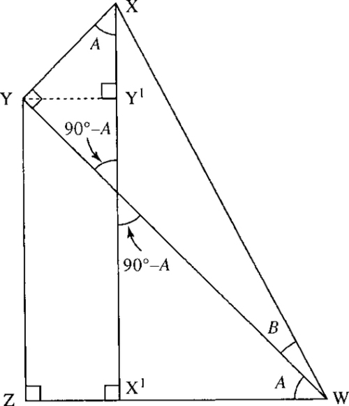
Looking at the triangles containing these sides we can see that this gives sin(A + B) = sin(A) cos(B) + cos(A) sin(B).
A similar argument can be used for cos(A + B), and tan(A + B) is usually found by using the expressions for sin(A + B), cos(A + B), and the definition of the tangent in terms of A and B.
![]()
Divide the top and bottom lines by cos(A) cos(B), giving

From these three identities for sin(A + B), cos(A + B), and tan(A + B) we can obtain many other expressions. A list of important trigonometric identities is given in Table 5.1.
Table 5.1
Summary of important trigonometric identities
| cos(A ± B) = cos(A) cos(B) ∓ sin(A) sin(B) |
| sin(A ± B) = sin(A) cos(B) ± cos(A) sin(B) |
tan(A ± B) =  |
sin(X) + sin(Y) = 2sin  cos cos |
| sin(X) − sin(Y) = 2cos |
| cos(X) + cos(Y) = 2cos |
| cos(X) − cos(Y) = −2sin |
| sin(2A) = 2sin(A)cos(A) |
| cos(2A) = cos2(A) − sin2(A) |
| tan(2A) = |
| cos(2A) = 2cos2(A) − 1 |
| cos(2A) = 1 − 2sin2(A) |
| cos2 (A) +sin2(A) = 1 |
| cos2(A) = |
| sin2(A) = |
| cos |
| sin |
Example 5.10
Using cos(2A) = cos2(A) – sin2(A) and cos2(A) + sin2(A) = 1, show that ![]()
Solution From cos2(A) + sin2(A) = 1, sin2(A) = 1 – cos2(A) (subtracting cos2(A) from both sides).
Substitute this into

Hence
![]()
Example 5.11
From
show that

Solution Use
and
and set
and
Using Equations (5.3) and (5.4), we can solve for A and B. Add Equations (5.3) and (5.4) giving
![]()
Subtract Equation (5.4) from Equation (5.3) giving
![]()
Add Equations (5.1) and (5.2) to give
sin(A + B) + sin(A – B) = sin(A) cos(B) + cos(A) sin(B)
⇔ sin(A) cos(B) – cos(A) sin(B)
⇔ sin(A + B) + sin(A − B) = 2 sin(A) cos(B).
Substitute for A and B giving

Example 5.12
Given that ![]()
![]()
and putting A = 30°, we get

From the knowledge of the graph of the cosine we know 
Example 5.13
Using sin(90°) = 1 and cos(90°) = 0, find sin(45°)
Solution Using
![]()
and putting A = 45°, 2A = 90°, we get

From the knowledge of the graph of the sine function we know that sin(45°) > 0, hence,
![]()
5.6 Superposition
The principle of superposition of waves states that the effect of a number of waves can be found by summing the disturbances that would have been produced by the individual waves separately. This behaviour is quite different from that of travelling particles, which will bump into each other, thereby altering the velocity of both.
The idea of superposition is used to explain the behaviour of:
1. stationary waves formed by two wave trains of the same amplitude and frequency travelling at the same speed in opposite directions.
2. Interference of coherent waves from identical sources.
3. Two wave trains of close frequency travelling at the same speed, causing beats.
4. Diffraction effects.
We look at some examples of these applications.
Standing waves
Suppose that a wave is created by plucking a string of a musical instrument; when the wave reaches the end of the string it is reflected back. The reflected wave will have the same frequency as the initial wave but a different phase and will be travelling in the opposite direction.
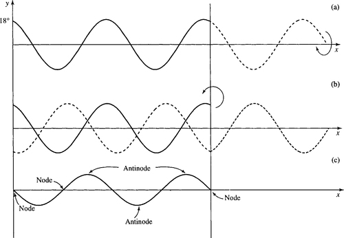
The sum of the incident and reflected wave forms a standing wave. An example is shown in Figure 5.18. Figure 5.18(a) shows the incident wave in a string at some instant in time. Its phase is 18°. Beyond the barrier is shown the hypothetical continuation of the wave as if there were no barrier. The reflected wave is found by turning this section upside down and reflecting it, as shown in Figure 5.18(b). The reflected wave has phase (180° – phase of the incident wave) = 180° − 18° = 162°. In Figure 5.18(c), the sum of the incident and reflected wave produces a standing wave. The maximum and minimum values on this are called antinodes and the zero values are called nodes. As the string is fixed at both ends there must be nodes at the ends.
At different moments in time, the phase of the incident wave will be different. This changes the amplitude of the standing wave but does not change the position of the nodes or antinodes (for a given frequency of wave). Only waves whose wavelengths exactly divide into 2l (twice the length of the string) can exist on the string because their amplitude must be 0 at the two end points. Each possible wavelength defines a mode of vibration of the string. λ = 2l is called the fundamental mode and is shown in Figure 5.19.

The standing wave can be explained using
![]()
The example given in Figure 5.18 has a wavelength of 4 giving wavenumber 360°/4 = 90°. The incident wave (phase 18°) is y = cos(90° x +18°) and the reflected wave is y = cos(90°x + 162°).
Summing these gives

As a 90° phase-shifted version of a cosine gives a negative sine, this gives −2cos(72°) sin(90°x). We see that the result is a sine wave of the same spatial frequency as the incident and reflected wave but with an amplitude of 2 cos 72° ≈ 0.62.
This result can also be found for a general situation – now expressing the phases, etc. in radians. The initial wave is cos (kx + δ) and the reflected wave is cos(kx + π – δ). The standing wave is given by summing these,
which gives
The standing wave has the same spatial frequency as the original waves. As cos(kx + π/2) = − sin(kx) and cos(δ – π/2) = sin(δ), this becomes −2 sin(kx) sin(δ). So, the instantaneous amplitude of the standing wave is 2 sin(δ) where δ is the phase of the incident wave.
5.7 Inverse trigonometric functions
From the graphs of the trigonometric functions, y = sin(x), y = cos(x), and y = tan(x), we notice that for any one value of y there are several possible values of x. This means that there are no inverse functions if all input values for x are allowed. However, we can see on a calculator that there is a function listed above the sine button and marked as sin−1, so is it in fact the inverse function?
Try the following with the calculator in degree mode. Enter 60 and press sin, then press sin−1. This is shown in Table 5.2(a). The same process is repeated for 120° and for −120°. However, for the latter two cases the inverse function does not work.
Table 5.2
sin and sin−1 on a calculator
| (a) | (b) | (c) | ||||||
| sin−1 | sin | sin−1 | sin | sin−1 | sin | |||
| 60° | → | 0.8660 | 120° | → | 0.8660 | −120° | → | −0.8660 |
| 60° | ← | 0.8660 | 60° | ← | 0.8660 | −60° | ← | −0.8660 |
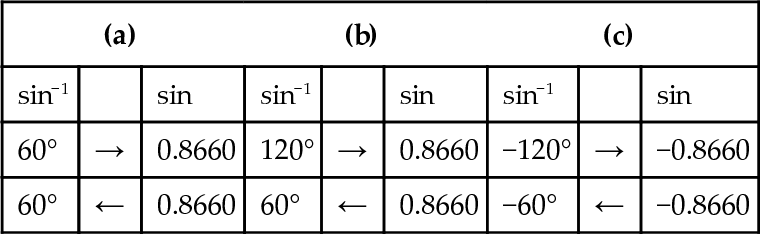
If we can restrict the range of values allowed into sin(x) to the range −90° to +90°, then sin−l (x) is a true inverse.
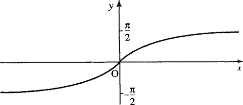
The inverse function of y = sin(x) is defined as f(x) = sin−1 (x) (often written as arcsin(x) to avoid confusion with 1/ sin(x)). It is the inverse function only if the domain of the sine function is limited to –π/2 ≤ x ≤ π/2. Thus, sin−l (sin(x)) = x if x lies within the limits given above and sin(sin−l (x)) = x if −1 ≤ x ≤ 1. The graph of y = sin−l (x) is given in Figure 5.20.

f(x) = cos−1 (x) is the inverse of y = cos(x) if the domain of cos(x) is limited to 0 ≤ x ≤ π. cos−l (cos(x)) = x if x is limited to the interval above and cos(cos−1 (x)) = x if −1 ≤ x ≤ 1. The graph of y = cos−1 (x) is given in Figure 5.21.

f(x) = tan−l (x) is the inverse of y = tan(x) if the domain of tan(x) is limited to –π/2 < x < π/2. Thus, tan−l (tan(x)) = x if x is limited as above and tan(tan−l(x)) = x for all x. The graph of y = tan−1 (x) is given in Figure 5.22.
5.8 Solving the trigonometric equations sin x = a, cos x= a, tan x = a
The solutions to the equations sin(x) = a, cos(x) = a, and tan (x) = a are shown in Figures 5.23–5.25, respectively. Where the lines y = a cross the sine, cosine, or tangent graph gives the solutions to the equations. In Figure 5.23, solutions to sin(x) = a are given by values of x where the line y = a crosses the graph y = sin(x). Notice that there are two solutions in every cycle. The first solution is sin−1 (a) and the second is given by π – sin −1 (a). Solutions in the other cycles can be found by adding a multiple of 2π to these two solutions.


In Figure 5.24, solutions to cos(x) = a are given by values of x where the line y = a crosses the graph y = cos(x). Notice that there are two solutions in every cycle. The two solutions in [− π, π] are cos −1 (a) and – cos −1 (a). Other solutions can be found by adding a multiple of 2π to these two solutions.
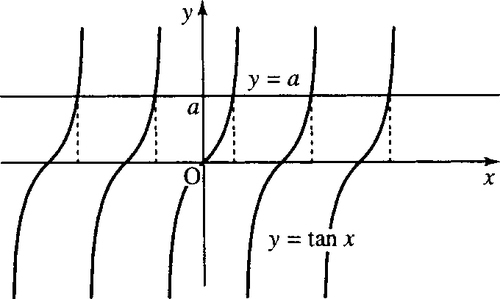
In Figure 5.25, solutions to tan(x) = a are given by values of x where the line y = a crosses the graph y = tan(x). Notice there is one solution in every cycle. The solution in [0, π] is tan−1 (a). Solutions in the other cycles can be found by adding a multiple of π to this solution.
Example 5.14
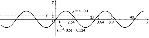
Find solutions to sin(x) = 0.5 in the range [2π, 4π]
Solution From the graph of y = sin(x) and the line y = 0.5 in Figure 5.26, the solutions can be worked out from where the two lines cross. The solution nearest x = 0 is given by sin−1(0.5) ≈ 0.524. The other solution in [0, 2π] is given by π − 0.524 ≈ 2.62. Any multiple of 2π added on to these solutions will also give a solution. Therefore, in the range [2π, 4π] the solutions are 3.64 and 8.9.
Example 5.15
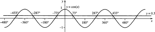
Find solutions to cos(x)= 0.3 in the range [−480°,480°].
Solution From the graph of y = cos(x) and the line y = 0.3 in Figure 5.27, the solutions can be worked out from where the two lines cross. The solution nearest x = 0 is given by cos−1 (0.3) ≈ 73°. The other solution in [0°, 360°] is given by −73°. Any multiple of 360° added on to these solutions will also give a solution. Therefore, in the range [−480°,480°] the solutions are −433°, −287°, −73°, 73°, 287°, and 433° (approximately).
Example 5.16
Find solutions to tan(x) = 0.1 in the range [360°, 540°].
Solution From the graph of y = tan(x) and the line y = 0.1 in Figure 5.28, the solutions can be worked out from where the two lines cross. The solution nearest x = 0 is given by tan−1(0.1) ≈ 6°. Any multiple of π added on to this solution will also give a solution. Therefore, in the range [360°, 540°] there is only one solution, that is, 366°.

5.9 Summary
1. Trigonometric functions can be defined using a rotating rod of length 1. The sine is given by plotting the height of the tip of the rod against the distance travelled. The cosine is given by plotting the position that the tip of the rod is to the left or right of the origin against the distance travelled. Hence, if the tip of the rod is at point (x, y) and the tip has travelled a distance of t units, then sin(t) = y, cos(t) = x, and the tangent is given by

2. If angles are measured in radians, then this definition is the same for angles between 0 and π/2 as that given by defining the cosine, sine, and tangent from the sides of a triangle (of hypotenuse 1) as
in Chapter 6 of the Background Mathematics Notes given on the companion website for this book.
There are 2π radians in a complete revolution (360°) and therefore π radians = 180°.
The trigonometric ratios can now be defined using a rotating rod of length r and the angle, α, made by the rod to the x axis. Then, if the tip of the rod is at point (x, y):
α is normally expressed in radians, although engineers often use degrees. If degrees are intended, then they must be explicitly marked.
3. sin(t) and tan(t) are odd functions, while cos(t) is an even function. This can be expressed by

sin(t) and cos(t) are periodic with period 2π and tan(t) is periodic with period π. This can be expressed by
where n ε ![]() .
.
4. For the function y = A cos(ax + b). A is the amplitude, the cycle rate (number of cycles in 1 unit) = a/2π, the fundamental period, or cycle length, P = 2π/α, the phase is b.
For a function of time y = A cos (ωt + ϕ), ω is the angular frequency and is measured in radians s−1. The number of cycles in
1 s is the frequency, f =ω/2π and is measured in Hz. The cycle length is called the periodic time or period (often represented by τ) = 2π/ω and is measured in seconds. The phase is ϕ.
For a function of distance y = A cos(kx + ϕ), k is the wavenumber. The number of cycles in 1 m is the spatial frequency, = k/2π wavelengths per metre, the cycle length is called the wavelength (often represented by λ) = 2π/k and is measured in metres, and the phase is ϕ.
The function y = A cos(ωt – kx) with t > 0 and ωt ≥ kx is called the progressive wave equation and has velocity v = λ f m s−1.
5. Wave amplitudes are often measured on a logarithmic scale using decibels.
6. There are many trigonometric identities, summarized on Table 5.1. Some of the more fundamental ones are:

from which others can be derived.
7. The principle of superposition of waves gives that the effect of a number of waves can be found by summing the disturbances that would have been produced by the waves separately. One application of this is the case of stationary waves, which can be explained mathematically using trigonometric identities.
8 sin−1 (x) is the inverse function to sin(x) if the domain of sin(x) is limited to –π/2≤x ≤ π/2, in which case sin−1 (sin(x)) = x.
cos−1 (x) is the inverse function to cos(x) if the domain of cos(x) is limited to 0 ≤ x ≤ π, in which case cos−1 (cos(x)) = x.
tan−1 (x) is the inverse function to tan(x) if the domain of tan(x) is limited to –π/2< x < π/2, in which case tan−1 (tan(x)) = x.
9. Inverse trigonometric functions are used in solving trigonometric equations. There are many solutions to trigonometric equations and graphs can be used to help see where the solutions lie.
sin(x) = a has two solutions: one is x = sin−1 (a) and another is π– sin−1 (a). Other solutions can be found by adding or subtracting a multiple of 2π.
cos(x) = a has two solutions: one is x = cos−1 (a) and another is – cos−1 (a). Other solutions can be found by adding or subtracting a multiple of 2π.
tan(x) = a has one solution: x = tan−1 (a). Other solutions can be found by adding or subtracting a multiple of π.
5.10 Exercises
5.1. Without using a calculator, express the following angles in degrees (remember π radians = 180°, π ≈3.142):
![]()
(b) 4π radians
(c)
![]()
(d) 6.284 radians
(e) 1.571 radians.
Check your answers using a calculator.
5.2 Without using a calculator, express the following angles in radians:
(b) 135°
(c) 10°
(d) 150°.
Check your answers using a calculator.
5.3. Given that cos(π/3) = 1/2, without using a calculator, find:
(b) tan(π/3)
(c) cos(2π/3)
(d) sin(7π/3)
(e) tan(4π/3)
Check your answers using a calculator.
5.4 By considering transformations of the graphs of sin(x), cos(x), and tan(x), sketch the graphs of the following:
(b) y = tan(x – (π/2))
(c) y = 3 sin(x)
(d) ![]()
(e) y = sin(πx)
(f)
![]()
(g) y = sin(x) + 3
(h) y = −cos(x).
5.5. From the graphs in Figure 5.29, find the phase, amplitude, period (cycle length), and number of cycles in one unit.

5.6. For the following functions of time, find the amplitude, period, angular frequency, and phase:
(b) V = sin(377t + 0.4)
(c) p = 40 cos(3000t − 0.8).
5.7. For the following functions of distance, x, find the amplitude, wavelength, spatial frequency, and wavenumber:
(b) y = 2 cos(72x + 0.33)
(c) y = 52 sin(80x)
5.8 Given a progressive wave t > 0

(a) Sketch the waves for t = 1, t = 5, and t = 10.
(b) Sketch the wave as a function of time for: (i) x = 2 (t > 5); and (ii) x = 4 (t > 10).
(c) Find the wave velocity and use your graphs to justify it.
5.9. A pneumatic drill produces a sound pressure of 6 N m−2. Given that the reference pressure is 2 × 10⁻⁵ N m−2, find the sound pressure level in decibels.
5.10. The reference level on a voltmeter is set as 0.775 V. Calculate the reading in decibels when the voltage reading is 0.4 V.
5.11. Show, using trigonometric identities, that
(a) cos(X + δ) – cos(X – δ) = −2 sin(δ) sin(X)
(b) sin(X + δ) + sin(X – δ) = 2 sin(X) cos(δ)
5.12. Two wave trains have very close frequencies and can be expressed by the sinusoids y = 2 sin(6.14t) and y = 2sin(6.19t). Their sum is sketched in Figure 5.30. Use the expression for the summation of two sines to find the beat frequency (the number of times the magnitude of the amplitude envelope reaches a maximum each second).

5.13. A single frequency of 200 Hz (message signal) is amplitude modulated with a carrier frequency of 2 MHz. Express the message signal as m = a cos (ω1t) and the carrier as c = b cos(ω2t) and assume that the modulation gives the product mc = ab cos(ω1t)cos(ω2t). Use trigonometric identities to show that the modulated signal can be represented by the sum of two frequencies at 2 × 10⁶ ± 200 Hz.
5.14
(a) Give the wavelengths of three modes of vibration on a string of length 0.75 m.
(b) The velocity v is approximately given by ![]() where T is the tension and m is the mass per unit length of the string. Given that T = 2200 N and m = 0.005 kg m−1 find the frequency of the fundamental mode.
where T is the tension and m is the mass per unit length of the string. Given that T = 2200 N and m = 0.005 kg m−1 find the frequency of the fundamental mode.
5.15. Use a cos(ωt+δ) = a cos(ωt) sin(δ)–a sin(ωt) sin(δ) to find c and d in the expression 2cos(3t + (π/3)) = c cos(3t)+ d sin(3t).
5.16. Express as single sines or cosines:
(a) sin(43°) cos(61°) + cos(43°) sin(61°)
(b) sin(22°) cos(18°) – cos(22°) cos(18°)
(c) cos(63°) cos(11°) + sin(63°) sin(11°)
(d) sin(41°) sin(22°) – cos(41°) cos(22°)
(e) sin(2x) cos(x) + cos(2x) sin(x)
(f) cos2(x) – sin2(x).
5.17. Express cos(x+y+z) in terms of the sines and cosines of x, y, and z.
5.18. Find all the solutions to the following equations in the interval [0, 6π]:
(b) tan(x) = 1/3
(c) cos(x) = −0.8
(d) sin2(x) = 0.25
(e) cos(x)+ 2cos2(x) = 0
(f) sin2(x) − 2 = 2.