
Probability and statistics
21.1 Introduction
Consider a system of computers and communication networks supporting a bank's cash dispensing machines. The machines provide instant money on the street on production of a cash card and a personal identification code with the only prerequisite being that of a positive bank balance.
The communication network must be reliable – that is, not subject too often to break downs. The reliability of the system, or each part of the system, will depend on each component part.
A very simple system, with only two components, can be configured in series or in parallel. If the components are in series then the system will fail if one component fails (Figure 21.1).

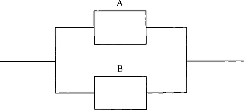
If the components are in parallel then only one component need function (Figure 21.2) and we have built in redundancy just in case one of the components fails.
A network could be made up of tens, hundreds, or even thousands of components. It is important to be able to estimate the reliability of a complex system and therefore the rate of replacement of components necessary and the overall annoyance level of our customers should the system fail.
The reliability will depend on the reliability of each one of the components but it is impossible to say exactly how long even one single component will last.
We would like to be able to answer questions like:
1. What is the likely lifetime of any one element of the system?
2. How can we estimate the reliability of the whole system by considering the interaction of its component parts?
This is just one example of the type of problem for which we need the ideas of probability and statistics. Others are, a factory produces 1000 electronic components each day where we wish to be able to estimate how many defective components are produced each day or a company with eight telephone lines where we wish to say whether that is a sufficient number, in general, for the number of calls likely to be received at any one time.
All of these questions are those that need the ideas of probability and statistics. Statistics is used to analyse data and produce predictions about it. Probability is the theory upon which statistical models are built.
For the engineering situations in previous chapters we have considered that we know all the factors that determine how a system will behave, that is, we have modelled the system deterministically. This is not very realistic. Any real situation will have some random element. Some problems, as the one we have just introduced, contain a large random element so that it is difficult to predict the behaviour of each part of the system. However, it is possible to say, for instance, what the average overall behaviour would be.
21.2 Population and sample, representation of data, mean, variance and standard deviation
In statistics, we are generally interested in a ‘population’ that is too large for us to measure completely. For instance, we could be interested in all the light bulbs that are produced by a certain manufacturer. The manufacturer may claim that her light bulbs have a lifetime of 1500 h. Clearly this cannot be exact but we might be satisfied to agree with the manufacturer if most of the bulbs have a lifetime greater than 1500 h. If the factory produces half a million light bulbs per year then we do not have the time to test them all. In this case we test a ‘sample’. The larger the sample, the more accurate will be the comparison with the whole population.
We have recorded the lifetimes of samples of light bulbs in Table 21.1. We can build up a table to give information about our sample. Columns 8 and 9 are given for comparison with statistical modelling and columns 4, 6, and 7 are to help with the calculation. The following describes each column of Table 21.1, beginning with a list of the ‘raw’ data.
Table 21.1
Frequency distribution of the lifetimes of a sample of light bulbs showing method of calculating the mean and standard deviation. N represents the number of classes, n the number in the sample
| (1) Lifetime (h) | (2) Class mid-point xi | (3) Class frequency fi | (4) fi(x) | (5) Cumulative frequency Fi | (6) (xi - | (7) fi(xi − | (8) Relative frequency fi /n | (9) Relative cumulative frequency Fi /n |
| 900–1000 | 950 | 2 | 1900 | 2 | 536849 | 1073698 | 0.002 | 0.002 |
| 1000–1100 | 1050 | 0 | 0 | 2 | 400309 | 0 | 0.002 | 0.002 |
| 1100–1200 | 1150 | 5 | 5750 | 7 | 283769 | 1418845 | 0.005 | 0.007 |
| 1200–1300 | 1250 | 23 | 28750 | 30 | 187229 | 4306267 | 0.023 | 0.03 |
| 1300–1400 | 1350 | 47 | 63450 | 77 | 110689 | 5202383 | 0.047 | 0.077 |
| 1400–1500 | 1450 | 103 | 149350 | 180 | 54149 | 5577347 | 0.103 | 0.18 |
| 1500–1600 | 1550 | 160 | 248000 | 340 | 17609 | 2817440 | 0.16 | 0.34 |
| 1600–1700 | 1650 | 190 | 313500 | 530 | 1069 | 203110 | 0.19 | 0.53 |
| 1700–1800 | 1750 | 165 | 288750 | 695 | 4529 | 747285 | 0.165 | 0.695 |
| 1800–1900 | 1850 | 164 | 303400 | 859 | 27989 | 4590196 | 0.164 | 0.859 |
| 1900–2000 | 1950 | 92 | 179400 | 951 | 71449 | 6573308 | 0.092 | 0.951 |
| 2000–2100 | 2050 | 49 | 100450 | 1000 | 134909 | 6610541 | 0.049 | 1 |
 |  | |||||||

Column 1: the class intervals
Find the minimum and the maximum of the data. The difference between these gives the range of the data. Choose a number of class intervals (usually up to about 20) so that the class range can be Chosen as some multiple of 10, 100, 1000, etc. (like the class range of 100 above). The data range divided by the class range and then rounded up to the integer above gives the number of classes. The class intervals are chosen so that the lowest class minimum is less than the minimum data value. In our example, the lowest class minimum has been chosen as 900. Add the class range of 100 to find the class interval, for example, 900–1000. Carryon adding the class range to find the next class interval until you pass the maximum value.
Column 2: the class midpoint
The class midpoint is found by the maximum value in the class interval – the minimum value in the class interval divided by 2. For the interval 1300–1400, the class midpoint is (1400 – 1300)/2 = 1350.
The class midpoint is taken as a representative value for the class. That is, for the sake of simplicity we treat the data in the class 1300–1400 as
though there were 47 values at 1350. This is an approximation that is not too serious if the classes are not too wide.
Column 3: class frequency and the total number in the sample
The class frequency is found by counting the number of data values that fall within that class range. For instance, there are 47 values between 1300 and 1400. You have to decide whether to include values that fall exactly on the class boundary in the class above or the class below. It does not usually matter which you choose as long as you are consistent within the whole data set.
The total number of values in the sample is given by the sum of the frequencies for each class interval.
Column 4: fixi and the mean of the sample, 
This is the product of the frequency and the class midpoint. If the class midpoint is taken as a representative value for the class then fixi gives the sum of all the values in that class. For instance, in the eighth class, with class midpoint 1650, there are 190 values. If we say that each of the values is approximately 1650 then the total of all the values in that class is 1650 × 190 = 313 500. Summing this column gives the approximate total value for the whole sample= 1 682 700 h. If we only used one light bulb at a time and changed it when it failed then the 1000 light bulbs would last approximately 1 682 700 h. The mean of the sample is this total divided by the number in the sample, 1000. Giving 1 682 700/1000 = 1682.7 h. The mean is a measure of the central tendency. That is, if you wanted a simple number to sum up the lifetime of these light bulbs you would say that the average life was 1683 h.
Column 5: the cumulative frequency
The cumulative frequency gives the number that falls into the current class interval or any class interval that comes before it. You could think of it as ‘the number so far’ function. To find the cumulative frequency for a class, take the number in the current class and add on the previous cumulative frequency for the class below, for example, for 1900–2000 we have a frequency of 92. The cumulative frequency for 1800–1900 is 859. Add 859 + 92 to get the cumulative frequency of 951. That is, 951 light bulbs in the sample have a lifetime below 2000 h. Notice that the cumulative frequency of the final class must equal the total number in the sample. This is because the final class must include the maximum value in the sample and all the others have lifetimes less than this.
Column 6: (Xi –  )2, the squared deviation
This column is used in the process of calculating the standard deviation (see column 7). (xi– ![]() ) represents the amount that the class midpoint differs from the mean of the sample. If we want to measure how spread out around the mean the data are, then this would seem like a useful number. However, adding up (xi–
) represents the amount that the class midpoint differs from the mean of the sample. If we want to measure how spread out around the mean the data are, then this would seem like a useful number. However, adding up (xi–![]() ) for the whole sample will just give zero, as the positive and negative values will cancel each other. Hence, we take the square, so that all the numbers are positive. For the sixth class interval the class midpoint is 1450; subtracting the mean, 1682.7, gives – 232.7, which when squared is 54149.2. This value is the square of the deviation from the mean, or just the squared deviation.
) for the whole sample will just give zero, as the positive and negative values will cancel each other. Hence, we take the square, so that all the numbers are positive. For the sixth class interval the class midpoint is 1450; subtracting the mean, 1682.7, gives – 232.7, which when squared is 54149.2. This value is the square of the deviation from the mean, or just the squared deviation.
Column 7: fi(xi −  )2, the variance and the standard deviation
For each class we multiply the frequency by the squared deviation, calculated in column 6. This gives an approximation to the total squared deviation for that class. For the sixth class we multiply the squared deviation of 54 149 by the frequency 103 to get 5 577 347. The sum of this column gives the total squared deviation from the mean for the whole sample. Dividing by the number of sample points gives an idea of the average squared deviation. This is called the variance. It is found by summing column 7 and dividing by 1000, the number in the sample, giving a variance of 39 120. A better measure of the spread of the data is given by the square root of this number, called the standard deviation and usually represented by σ. Here ![]() .
.
Column 8: the relative frequency
If instead of 1000 data values in the sample we had 2000, 10 000, or 500, we might expect that the proportion falling into each class interval would remain roughly the same. This proportion of the total number is called the relative frequency and is found by dividing the frequency by the total number in the sample. Hence, for the third class, 1100–1200, we find 5/1000 = 0.005.
Column 9: the cumulative relative frequency
By the same argument as above we would expect the proportion with a lifetime of less than 1900 h to be roughly the same whatever the sample size. This cumulative relative frequency can be found by dividing the cumulative frequency by the number in the sample. Notice that the cumulative relative frequency for the final class interval is 1. That is, the whole of the sample has a lifetime of less than 2000 h.
The data can be represented in a histogram as in Figure 21.3, which gives a simple pictorial representation of the data. The right-hand side has a scale equal to the left-hand scale divided by the number in the sample. These readings, therefore, give the relative frequencies and the cumulative relative frequency as given in Table 21.1.

We may want to sum up our findings with a few simple statistics. To do this we use a measure of the central tendency and the dispersion of the data, which are calculated as already described above. These are summarized below.
Central tendency – the mean
The most commonly used measure of the central tendency is the mean, ![]()
![]()
where xiis a representative value for the class and fiis the class frequency. The summation is over all classes.
If the data have not been grouped into classes then the mean is found by summing all the individual data values and dividing by the number in the sample:
![]()
where the summation is now over all sample values
Dispersion – the standard deviation
The variance is the mean square deviation given by
![]()
where ![]() is the sample mean, xiis a representative value for the class, fiis the class frequency, and the summation is over all classes. This value is the same as
is the sample mean, xiis a representative value for the class, fiis the class frequency, and the summation is over all classes. This value is the same as
![]()
which can some times be quicker to calculate.
For data not grouped into classes we have
![]()
or
![]()
where the summation is now over all sample values.
The standard deviation is given by the square root of the variance:
![]()
We have already calculated the average lifetime and the standard deviation of the lifetimes of the sample of light bulbs. We repeat the calculation below. The mean is given by
The variance is given by
Hence, the standard deviation is
![]()
Can we agree with the manufacturer's claim that the light bulbs have a lifetime of 1500 h? The number with a lifetime of less than 1500 h is 180 (the cumulative frequency up to 1500 h). This represents only 0.18, less than 20% of the sample. However, this is probably an unreasonable number to justify the manufacturers claim as nearly 20% of the customers will get light bulbs that are not as good as advertised. We might accept a small number, say 5%, failing to live up to a manufacturer's promise. Hence, it would be better to claim a lifetime of around 1350 h with a relative cumulative frequency between 0.03 and 0.077. Approximately 0.053 or just over 5% would fail to live up to the manufacturer's amended claim.
Example 21.1
A sample of 2000-Ω resistors were tested and their resistances were found as below:
Group the data in class intervals and represent it using a table and a histogram. Calculate the mean resistance and the standard deviation.
Solution We follow the method of building up the table as described previously.
Column 1: class intervals. To decide on class intervals look at the range of values presented. The minimum value is 1995 and the maximum is 2006. A reasonable number of class intervals would be around 10, and in this case as the data are presented to the nearest whole number, the smallest possible class range we could choose would be 1 Ω. A 1-Ω class range would give 12 classes, which seems a reasonable choice. If we choose the class midpoints to be the integer values then we get class intervals of 1994.5–1995.5, 1995.5–1996.5, etc. We can now produce Table 21.2.
Table 21.2
Frequency distribution of resistances of a sample of resistors. N represents the number of classes, n the number in the sample
| (1) Resistance (Ω) | (2) Class mid-point xi | (3) Class frequency fi | (4) fi (x) | (5) Cumulative frequency Fi | (6) (xi - | (7) fi(xi −x)2 | (8) Relative frequency fi /n | (9) Relative cumulative frequency Fi/n |
| 1994.5–1995.5 | 1995 | 1 | 1995 | 1 | 26.52 | 26.52 | 0.01 | 0.01 |
| 1995.5–1996.5 | 1996 | 3 | 5988 | 4 | 17.22 | 51.66 | 0.03 | 0.04 |
| 1996.5–1997.5 | 1997 | 5 | 9985 | 9 | 9.92 | 49.6 | 0.05 | 0.09 |
| 1997.5–1998.5 | 1998 | 13 | 25974 | 22 | 4.62 | 60.06 | 0.13 | 0.22 |
| 1998.5–1999.5 | 1999 | 17 | 33983 | 39 | 1.32 | 22.44 | 0.17 | 0.39 |
| 1999.5–2000.5 | 2000 | 19 | 38000 | 58 | 0.02 | 0.38 | 0.19 | 0.58 |
| 2000.5–2001.5 | 2001 | 16 | 32016 | 74 | 0.72 | 11.52 | 0.16 | 0.74 |
| 2001.5–2002.5 | 2002 | 15 | 30030 | 89 | 3.42 | 51.3 | 0.15 | 0.89 |
| 2002.5–2003.5 | 2003 | 4 | 8012 | 93 | 8.12 | 32.48 | 0.04 | 0.93 |
| 2003.5–2004.5 | 2004 | 4 | 8016 | 97 | 14.82 | 59.28 | 0.04 | 0.97 |
| 2004.5–2005.5 | 2005 | 2 | 4010 | 99 | 24.52 | 47.04 | 0.02 | 0.99 |
| 2005.5–2006.5 | 2006 | 1 | 2006 | 100 | 34.22 | 34.22 | 0.01 | 1 |
 |  | |||||||
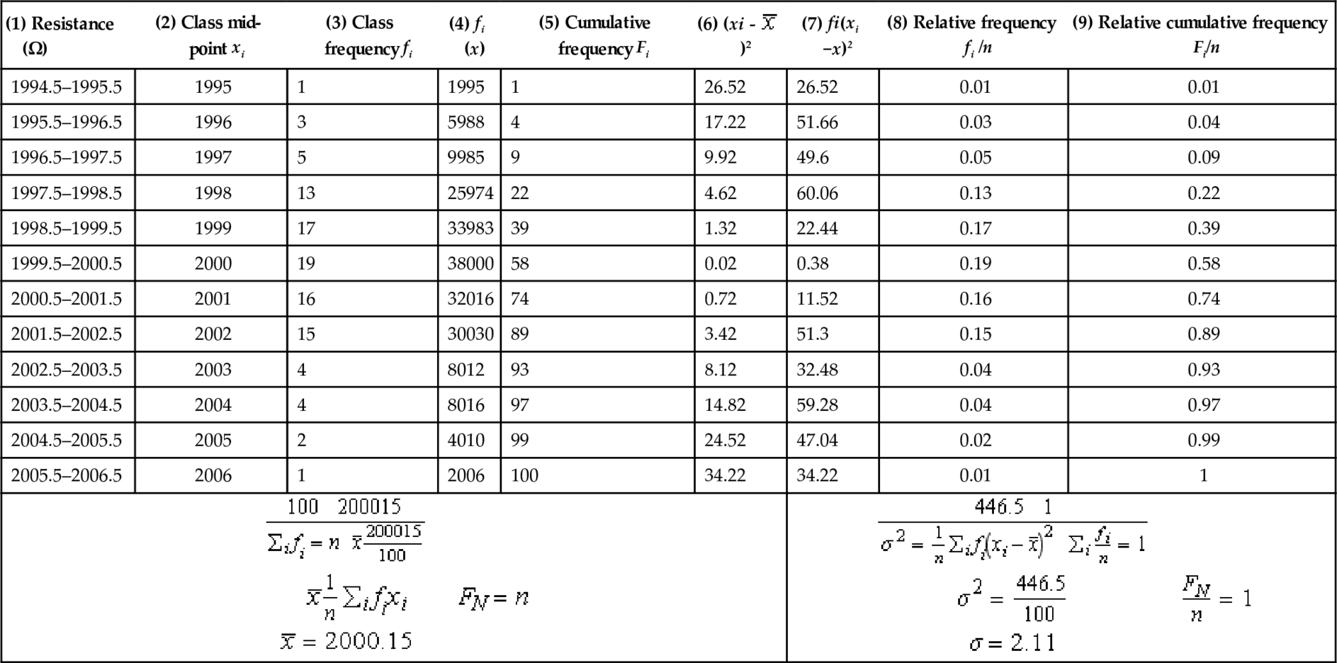
The other columns are filled in as follows:
Column 2. To find the frequency, count the number of data values in each class interval. The sum of the frequencies gives the total number in the sample; in this case 100.
Column 3. The cumulative frequency is given by adding up the frequencies so far. The number of resistances up to 1995.5 is 1. As there are three in the interval 1995.5–1996.5, add 1 + 3 = 4 to get the number up to a resistance of 1996.5. The number up to 1997.6 is given by 4 + 5 = 9, etc.
Column's 4, 6, and 7 help us calculate the mean and standard deviation. To find column 4 multiply the frequencies (column 3) by the class midpoints (column 2) to get fixi.
The sum of this column is an estimate of the total if we added all the values in the sample together. Therefore, dividing by the number of items in the sample gives the mean:
To find the standard deviation we calculate the variance first. The variance is the mean squared deviation. Find the difference between the mean and each of the class intervals and square it. This gives column 6. Multiply by the class frequency to get column 7. Finally, add them all up and divide by the total number. This gives the variance:
![]()
and the standard deviation
![]()
The relative frequency (given in column 8) is the fraction in each class interval; that is, the frequency divided by the total number. For example, the relative frequency in the class interval 2000.5–2001.5 is 16/100 = 0.16
The cumulative relative frequency is the cumulative frequency divided by the total number n. The cumulative frequency up to 2000.5 is 58. Divided by the total number gives 0.58 for the relative cumulative frequency.
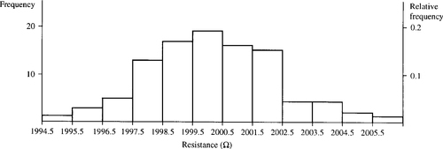
We can sum up this sample by saying that the mean resistance is 2000.15 with a standard deviation of 2.11. These simple figures can be used to sum up how closely the claim that they are resistors of 2000Ω can be justified. We can also picture the frequency distribution using a histogram as in Figure 21.4
Returning to the lifetimes of the light bulbs we might want to ask what average lifetime and standard deviation might lead to less than 5% of the light bulbs having a lifetime less than 1500 h?
To answer this sort of problem we need to build up a theory of statistical models and use probability theory.
21.3 Random systems and probability
We are dealing with complicated systems with a number of random factors affecting its behaviour; for instance, those that we have already seen, production of resistors, lifetimes of bulbs. We cannot determine the exact behaviour of the system but using its frequency distribution we can estimate the probabilities of certain events.
Relative frequency and probability
The probability of an event is related to its relative frequency. If I chose a light bulb from the sample in Section 21.2, then the probability of its lifetime being between 1400 and 1500 h is 0.103. This is the same as the relative frequency for that class interval, that is, the number in the class interval divided by the total number of light bulbs in the sample. Here, we have assumed that we are no more likely to pick any one light bulb than any other, that is, each outcome is equally likely. The histogram of the relative frequencies (Figure 21.3 using the right-hand scale) gives the probability distribution function (or simply the probability function) for the lifetimes of the sample of light bulbs.
As an introduction to probability, examples are often quoted involving throwing dice or dealing cards from a pack of playing cards. These are used because the probabilities of events are easy to justify and not because of any particular predilection on the part of mathematicians to a gambling vocation!
Example 21.2
A die has the numbers one to six marked on its sides. Draw a graph of the probability distribution function for the outcome from one throw of the die, assuming it is fair.
Solution If we throw the die 10 000 times we would expect the number of times each number appeared face up to be roughly the same. Here, we have assumed that the die is fair; that is, any one number is as likely to be thrown as any other. The relative frequencies would be approximately 1/6. The probability distribution function, therefore, is a flat function with a value of 1/6 for each of the possible outcomes of 1,2,3,4,5,6. This is shown in Figure 21.5

Notice two important things about the probabilities in the probability distribution for the die:
1. each probability is less than 1;
2. the sum of all the probabilities is 1:
![]()
Example 21.3
A pack of cards consists of four suits, hearts, diamonds, spades, and clubs. Each suit has 13 cards; that is, cards for the numbers 1 (the ace) to 10 and a Jack, Queen, and King. Draw a graph of the probability distribution function for the outcome when dealing one card from the pack, where only the suit is recorded. Assume the card is replaced each time and the pack is perfectly shuffled.
Solution If a card is selected, the suit recorded hearts, spades, clubs, or diamonds, the card is placed back in the pack and the pack is shuffled. If this is repeated (say 10 000 times) then we might expect that each suit will occur as often as any other, that is, 1/4 of the time. The probability distribution function again is a flat distribution, and has the value of 1/4 for each of the possible four outcomes. The probability distribution for suits is given in Figure 21.6.

Notice again that in Example 21.3 each probability is less than 1 and that the sum of all the probabilities is 1:
![]()
We have seen that a probability distribution can be represented using a graph. Each item along the x-axis has an associated probability. Probability is a function defined on some set. The set is called the sample space, S, and contains all possible outcomes of the random system. The probability distribution function is often abbreviated to p.d.f.
Some definitions
A trial is a single observation on the random system, for example, one throw of a die, one measurement of a resistance in the example in Section 21.2.
The sample space is the set of all possible outcomes, for example, for the die it is the set {1, 2, 3, 4, 5, 6}, and for the resistance problem it is the set of all possible measured resistances. This set may be discrete or continuous. An event is a set of outcomes. For instance, A is the event of throwing less than 4 and B is the event of throwing a number greater than or equal to 5.
An event is a subset of the sample space S.
Notice that in the case of a continuous sample space an event is also a continuous set, represented by an interval of values. For example, C is the event that the resistance lies in the interval 2000 ± 1.5.
Probability
The way that probability is defined is slightly different for the case of a discrete sample space or a continuous sample space.
Discrete sample space
The outcome of any trial is uncertain; however, in a large number of trials the proportion showing a particular outcome approaches a certain number. We call this the probability of that outcome. The probability distribution function, or simply probability function, gives the value of the probability that is associated with each outcome. The probability function obeys two important conditions:
1. all probabilities are less than, or equal to 1, that is, ![]() where x is any outcome in the sample space;
where x is any outcome in the sample space;
2. the probabilities of the individual outcomes sum to 1, that is, ∑ p(x) = 1.
Continuous sample space
Considering a continuous sample space. We assign probabilities to intervals. We find the probability of, for instance, the resistance being in the interval 2000 ± 0.5. Hence, we assign probabilities to events and not to individual outcomes. In this case, the function that gives the probabilities is called the probability density function and we can find the probability of some event by integrating the probability density function over the interval. For instance, if we have a probability density function f (x), where x can take values from a continuous sample space, then the probability of x being in the interval a to b is given by, for example,
![]()
The probability density function obeys the condition:
![]()
that is, the total area under the graph of the probability density function must be 1.
Equally likely events
If all outcomes are equally likely then the probability of an event E from a discrete sample set is given by
![]()
That is, the probability of E is equal to the proportion of the whole sample space that is in E, when each of the outcomes are equally likely.
Example 21.4
What is the probability on one throw of a die getting a number less than 3?
Solution Give this event the name A. Then A = { 1, 2} and S = {1,2,3,4,5, 6}. The number in A is 2 and the number in S is 6. Therefore, as each outcomes is equally likely, p(A), the probability of A is 2/6 = 1/3.
This particular result leads to another way of representing probability – by using area.
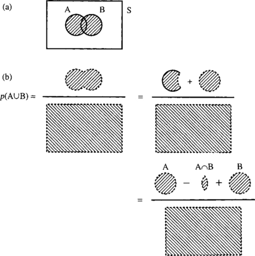
If we use a rectangle to represent the set of all possible outcomes, S, then an event is a subset of S, that is, one section of the rectangle and if all outcomes are equally likely then its probability can be pictured by the proportion of S that is in A. We will put a dotted line around the picture representing the set A to indicate the number in A or the area of A (see Figure 21.7).

This way of picturing the probability of an event can help in remembering some of the probabilities of combined events.
21.4 Addition law of probability
Disjoint events
Disjoint events are events with no outcomes in common. They cannot happen simultaneously.
Example 21.5
A is the event that a card chosen from a playing pack is under 6 (counting ace as low, i.e. = 1) and B is the event of choosing a picture card (Jack, Queen, or King). Find the probability that a card chosen from the pack is under 6 or is a picture card.
Solution
A and B are disjoint. As each outcome is considered to be equally likely the probabilities are easy to find:
![]()
There are 52 cards; therefore, 52 possible outcomes in S, so
![]()
Also
![]()
We want to find the probability of A or B happening; that is, the probability that the card is either under 6 or is a picture card:
We can see that:
We can also see this by using the idea of area to picture it, as in Figure 21.8.

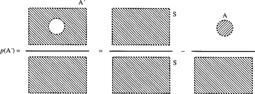
We can also consider the probability of A not happening; that is, the probability of the complement of A, which we represent by A′. As A and A′ are disjoint.
![]()
This is shown in Figure 21.9.
Non-disjoint events
Example 21.6
Consider one throw of a die
![]()
Find the probability that the result of one throw of the die is either an even number or a multiple of 3.
Solution
![]()
then
and

and
![]()
Looking at the problem and using the idea of areas in the set, we can see from Figure 21.10 that the rule becomes
![]()
21.5 Repeated trials, outcomes, and probabilities
Supposing we start to consider more complicated situations, like throwing a die twice. Then the outcomes can be found by considering all the possible outcomes of throwing the die the first time combined with all the possible outcomes of throwing the die the second time. As there are six possible outcomes for the first throw and six possible outcomes for the second throw, then there are 6 × 6 = 36 outcomes of throwing the die twice.
If we would like to find the probability that the first throw is a 5 and the second throw is a 5 or 6 then we can do this by listing all the 36 outcomes and finding the proportion that fall into our event.
The set S of all possible outcomes has 36 elements:
and each has an equally likely outcome. E = the first throw is a 5 and the second is a 5 or 6. Hence
![]()
![]()
This sort of problem can be pictured more easily using a probability tree.
21.6 Repeated trials and probability trees
Repeatedly tossing a coin
The simplest sort of trial to consider is one with only two outcomes; for instance, tossing a coin. Each trial has the outcome of head or tail and each is equally likely.
We can picture repeatedly tossing the coin by drawing a probability tree. The tree works by drawing all the outcomes and writing the probabilities for the trial on the branches. Let us consider tossing a coin three times. The probability tree for this is shown in Figure 21.11.

There are various rules and properties we can notice.
Rules of probability trees and repeated trials
1. The probabilities of outcomes associated with each of the vertices can be found by multiplying all the probabilities along the branches leading to it from the top of the tree. HTH has the probability
![]()
2. At each level of the tree, the sum of all the probabilities on the vertices must be 1.
3. The probabilities along branches out of a single vertex must sum to 1. For example, after getting a head on the first trial we have a probability of 1/2 of getting a head on the second trial and a probability of 1/2of getting a tail. Together they sum to 1.
The fourth property is one that is only true when the various repeated trials are independent, that is, the result of the first trial has no effect on the possible result of the second trial, etc.
4. For independent trials, the tree keeps repeating the same structure with the same probabilities associated with the branches. Here, the event of getting a head on the third toss is independent of the event of getting a head on the first or second toss.
Using the tree we can find various probabilities, as we see in Example 21.7.
Example 21.7
What is the probability on three tosses of the coin that exactly two of them will be heads?
Solution Count up all the ways that we could have two heads and one tail, looking at the foot of the probability tree in Figure 21.11. We find three possibilities:
![]()
each of these has probability of ![]() Therefore, the probability of exactly two heads is
Therefore, the probability of exactly two heads is ![]()
Picking balls from a bag without replacement
We have 20 balls in a bag. Ten are red and ten are black. A ball is picked out of the bag, its colour recorded and then it is not replaced into the bag. There are two possible outcomes of each trial, red (R) or black (B). Let us consider three trials and their associated outcomes in a probability tree, as shown in Figure 21.12.

To find the probabilities we consider how many balls remain in each case. If the first ball chosen is red then there are only 19 balls left of which 9 are red and 10 are black; therefore, the probability of picking a red ball on the second trial is only 9/19 and the probability of picking black is 10/19.
The first three rules given in the last example apply.
1. The probabilities of outcomes associated with each of the vertices can be found by multiplying all the probabilities along the branches leading to it from the top of the tree. BRB has the probability:
![]()
2. At each level of the tree the sum of all the probabilities on the vertices must be 1; for example, at the second level we have
![]()
3. The probabilities along branches out of a single vertex must sum to 1; for example, after picking red on the first trial we have a probability of 9/19 of picking red and 10/19 of picking black. Together they sum to 1.
The fourth property is no longer true as the various repeated trials are not independent. The result of the first trial has an effect on the possible result of the second trial, etc.
Using the tree we can find the probability of various events as in Example 21.8.
Example 21.8
Of 20 balls in a bag 10 are red and 10 are black. A ball is picked out of the bag, its colour recorded and then it is not replaced into the bag. What is the probability that of the first three balls chosen exactly two will be red?
Solution We can use the probability tree in Figure 21.12 to solve this problem. We look at the foot of the tree, which gives all the possible outcomes after three balls have been selected.
The ways of getting two red are RRB, RBR, BRR and the associated probabilities are
![]()
or
![]()
Summing these gives the probability of exactly two reds being chosen out of the three as 30/76.
21.7 Conditional probability and probability trees
The probabilities we have been writing along the branches of the probability tree are called conditional probabilities.
Example 21.9
What is the probability that the first throw of a die will be a 5 and the second throw will be a 5 or 6?
Solution A is the set of those outcomes with the first throw a 5 and B is the set of those outcomes with the second throw a 5 or 6. We can use a probability tree in the following way. After the first throw of the die either A is true or not, that is, we have only two possibilities, A or A'. After that, we are interested in whether B happens or not. Again we either get B or B’. We get the probability tree as in Figure 21.13.

Here, p(B|A) means the probability of B given A, similarly p(B|A′) means the probability of B given (not A). We can fill in the probabilities using our knowledge of the fair die. The probability of A is 1/6. The second throw of the die is unaffected by the throw first throw of the die; therefore
![]()
Working out the other probabilities gives the probability tree in Figure 21.14.

The probability that the first throw of a die will be a 5 and the second throw will be a 5 or 6 is p(B∩A), given from the tree in Figure 21.14 as
![]()
Notice that the probability we have calculated is the intersection of the two events A and B, that is, we calculated the probability that both occurred. When multiplying the probabilities on the branches of the probability tree we are using the following:
![]()
Furthermore, because of independence we have used the fact that p(B|A) = p(B). That is, the probability of B does no depend on whether A has happened or not: B is independent of A. We, therefore, have the following important results.
Multiplication law of probability
![]()
This law applies for any two events A and B. It is the law used in finding the probabilities of the vertices of the probability trees.
Example 21.10
It is known that 10% of a selection of 100 electrical components are faulty. What is the probability that the first two components selected are faulty if the selection is made without replacement?
Solution The probability we are looking for is:
p(first faulty ∩ second faulty)
= p(first faulty) p(second faulty | first faulty)
Here there are only two possibilities at each stage, faulty or not faulty. The probability tree is as shown in Figure 21.15.

Notice that their are only 99 components left after the first trial and whether the first was faulty or not changed the probability that the second is faulty or otherwise. Each branch of the tree, after the first layer, represents a conditional probability.
The answer to our problem is therefore

Condition of independence
If two events A and B are independent then
![]()
Notice that the multiplication law changes in this case, as described below.
Multiplication law of probability for independent events
![]()
There is one other much-quoted law of probability that completes all the basic laws from which probabilities can be worked out. That is Bayes's theorem and it comes from the multiplication law.
Bayes's theorem
As p(A ∩ B) = p(A) p(B|A) then as A ∩ B = B ∩ A we can also write p(B ∩ A) = p(B) p(A|B) and putting the two together gives p(A) p(B|A) = p(B) p(A|B) or
![]()
Bayes's theorem is important because it gives a way of swapping conditional probabilities that may be useful in diagnostic situations where not all of the conditional probabilities can be found directly.
Example 21.11
In a certain town there are only two brands of hamburgers available, Brand A and Brand B. It is known that people who eat Brand A hamburger have a 30% probability of suffering stomach pain and those who eat Brand B hamburger have a 25% probability of suffering stomach pain. Twice as many people eat Brand B compared to Brand A hamburgers. However, no one eats both varieties. Supposing one day you meet someone suffering from stomach pain who has just eaten a hamburger, what is the probability that they have eaten Brand A and what is the probability that they have eaten, Brand B?
Solution First we define the sample space S, and the other simple events.
S = people who have just eaten a hamburger
A = people who have eaten a Brand A hamburger
B = people who have eaten a Brand B hamburger
C = people who are suffering stomach pains
We are given that:

Note also that S = A ∪ B.
As those who have stomach pain have either eaten Brand A or B, then A ∩ B = Ø

Then
![]()
and
![]()
Hence, if they have stomach pain the probability that they have eaten Brand A is 3/8 and the probability that they have eaten Brand B is 5/8.
21.8 Application of the probability laws to the probability of failure of an electrical circuit
Components in series
We denote ‘The probability that A does not fail’ as p(A). Then the probability that S fails is p(S’) = 1 – p(S).
As they are in series (see Figure 21.16), S will function if both A and B function: S = A ∩ B. Therefore
![]()

as A and B are independent
![]()
Example 21.12
An electrical circuit has three components in series (see Figure 21.17). One has a probability of failure within the time of operation of the system of 1/5; the other has been found to function on 99% of occasions and the third component has proved to be very unreliable with a failure once for every three successful runs. What is the probability that the system will fail on a single operation run.

Solution Using the method of reasoning above we call the components A, B, and C. The information we have is
The probability we would like to find is p(S’), the probability of failure of the system and we know that the system is in series so S = A ∩ B ∩ C; that is, all the components must function for the system to function. We can find the probability that the system will function and subtract it from 1 to find the probability of failure:
![]()
As all the components are independent,
![]()
We can find p(A), p(B), and p(C) from the information we are given: p(A) = 1 – p(A’) = 1 −1/5 = 0.8 and p(B) is given as 0.99.
Given that p(C') : p(C) = 1 : 3, C fails once in every 1 + 3 occasions, so p(C') = 1/4 = 0.25 and p(C) = 1 – p(C') = 0.75.
We can now find p(A)p(B)p(C) = 0.8 × 0.99 × 0.75 = 0.594. This is the probability that the system will function, so the probability it will fail is given by 1 – 0.594 = 0.406.
Components in parallel
If a system S consists of two components A and B in parallel, as in Figure 21.18, then S fails if both A and B fail.
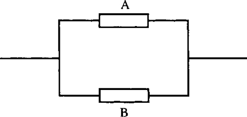
Again denote ‘The probability that A does not fail’ as p(A). Then the probability that S fails is
![]()
As they are in parallel, S will function if either A or B functions: S = A ∪ B. Therefore
![]()
A and B are independent, but not disjoint. They are not disjoint because both A and B can function simultaneously. From the addition law of probabilities given in Section 21.4
![]()
As A and B are independent,
![]()
Therefore

As this is a long-winded expression it may be more useful to look at the problem the other way round. S fails only if both A and B fail: S' = A' ∩B'. So
![]()
as A and B are independent. Finally, p(S′) = p(A’) p(B’).
This is a simpler form that we may use in preference to the previous expression we derived. It must be equivalent to our previous result, so we should just check that by substituting p(A') = 1 – p(A) and p(B') = 1 – p(B). Hence

which is the same as we had before.
Let us try a mixed example with some components in series and others in parallel.
Example 21.13
An electrical circuit has three components, two in parallel, components A and B, and one in series, component C. They are arranged as in Figure 21.19. Component's A and B are identical components with a 2/3 probability of functioning and C has a probability of failure of 0.1%. Find the probability that the system fails.

Solution We denote ‘The probability that A functions’ as p(A). The information we have is

The probability we would like to find is p(S‘), the probability of failure of the system and we know that the system will function if (either A or B function) and C functions. So
![]()
From the multiplication law for independent events we have:
![]()
From the addition law for non-disjoint events (A and B are not disjoint because both A and B can occur), we have:
![]()
![]()
So p(S) = p (A ∪ B) p(C) = 0.8889 × 0.999 = 0.888. Hence, the probability that the system functions is 0.888.
21.9 Statistical modelling
Suppose, as in Example 21.2, we have tested 5000 resistors and recorded the resistance of each one to an accuracy of 0.01Ω. We may wish to quickly decide whether the manufacturers claim of producing 2000-Ω resistors is correct. One way of doing this is to divide our resistors into class intervals and draw up a table and a histogram. We can then count the percentage of resistors that are outside of acceptable limits and assume that the population behaviour is the same as the sample behaviour. Hence, if 98% of the resistors lie between 2000 ± 0.1% we may be quite happy.
A quicker way of doing this is to use a statistical model. That is, we can guess what the histogram would look like based on our past experience. To use such a model we probably only need to know the population mean, μ, and the population standard deviation, σ.
In the rest of this chapter, we will look at four possible ways of modelling data, the normal distribution, the exponential distribution, both continuous models, and the binomial distribution and the Poisson distribution which are discrete models.
21.10 The normal distribution
The normal distribution is symmetric about its mean. It is bell-shaped and the fatness of the bell depends on its standard deviation. Examples are given in Figure 21.20 and 21.21.

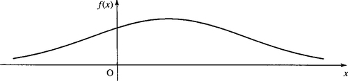
The normal distribution is very important because of the following points:
1. Many practical distributions approximate to the normal distribution. Look at the histograms of lifetimes given in Figure 21.3 and of resistances given in Figure 21.4 and you will see that they resemble the normal distribution. Another common example is the distribution of errors. If you were to get a large group of students to measure the diameter of a washer to the nearest 0.1 mm, then a histogram of the results would give an approximately normal distribution. This is because the errors in the measurement are normally distributed.
2. The central limit theorem. If we take a large number of samples from a population and calculate the sample means then the distribution of the sample means will behave like the normal distribution for all populations (even those populations which are not distributed normally). This is as a result of what is called the central limit theorem. There is a project exploring the behaviour of sample means given in the Projects and Investigations available on the companion website for this book.
3. Many other common distributions become like the normal distribution in special cases. For instance, the binomial distribution, which we shall look at in Section 21.12, can be approximated by the normal when the number of trials is very large.
Finding probabilities from a continuous graph
Before we look at the normal distribution in more detail we need to find out how to relate the graph of a continuous function to our previous idea of probability. In Section 21.3, we identified the probability of a class with its relative frequency in a frequency distribution. That was all right when we had already divided the various sample values into classes. The problem with the normal distribution is that is has no such divisions along the x-axis and no individual class heights, just a nice smooth curve.
To overcome this problem we define the probability of the outcome lying in some interval of values, as the area under the graph of the probability function between those two values as shown in Figure 21.22.
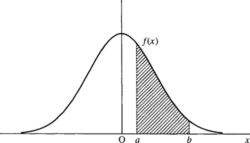
As we found in Chapter 7, the area under a curve is given by the integral; therefore, for a continuous probability distribution, f (x), we define
![]()
The cumulative distribution function gives us the probability of this value or any previous value (it is like the cumulative relative frequency). A continuous distribution thus becomes the ‘the area so far’ function and therefore becomes the integral from the lowest possible value that can occur in the distribution up to the current value.
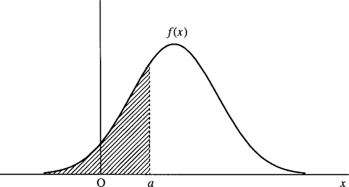
The cumulative distribution up to a value a is represented by
![]()
and it is the total area under to graph of the probability function up to a; this is shown in Figure 21.23.
We can also use the cumulative distribution function to represent probabilities of a certain interval. The area between two values can be found by subtracting two values of the cumulative distribution function as in Figure 21.24.

However, there is a problem with the normal distribution function in that is not easy to integrate! The probability density function for x, where x is N(μ σ2) is given by
![]()
It is only integrated by using numerical methods. Hence, the values of the integrals can only be tabulated. The values that we have tabulated are the areas in the tail of the standardized normal distribution; that is
![]()
where f (z) is the probability distribution with 0 mean (μ = 0) and standard deviation of 1 (σ = 1). This is shown in Figure 21.25 and tabulated in Table 21.3. In order to use these values we need to use ideas of transformation of graphs from Chapter 2 to transform any normal distribution into its standardized form.


Table 21.3
Areas in the tail of the standardized normal distribution. P(z > u) values are given where z is a variable with distribution N(0, 1)
| u | 0.00 | 0.01 | 0.02 | 0.03 | 0.04 | 0.05 | 0.06 | 0.07 | 0.08 | 0.09 |
| 0.0 | 0.50000 | 0.49601 | 0.49202 | 0.48803 | 0.48405 | 0.48006 | 0.47608 | 0.47210 | 0.46812 | 0.46414 |
| 0.1 | 0.46017 | 0.45620 | 0.45224 | 0.44828 | 0.44433 | 0.44038 | 0.43644 | 0.43251 | 0.42858 | 0.42465 |
| 0.2 | 0.42074 | 0.41683 | 0.41294 | 0.40905 | 0.40517 | 0.40129 | 0.39743 | 0.39358 | 0.38974 | 0.38591 |
| 0.3 | 0.38209 | 0.37828 | 0.37448 | 0.37070 | 0.36693 | 0.36317 | 0.35942 | 0.35569 | 0.35197 | 0.34827 |
| 0.4 | 0.34458 | 0.34090 | 0.33724 | 0.33360 | 0.32997 | 0.32636 | 0.32276 | 0.31918 | 0.31561 | 0.31207 |
| 0.5 | 0.30854 | 0.30503 | 0.30153 | 0.29806 | 0.29460 | 0.29116 | 0.28774 | 0.28434 | 0.28096 | 0.27760 |
| 0.6 | 0.27425 | 0.27093 | 0.26763 | 0.26435 | 0.26109 | 0.25785 | 0.25463 | 0.25143 | 0.24825 | 0.24510 |
| 0.7 | 0.24196 | 0.23885 | 0.23576 | 0.23270 | 0.22965 | 0.22663 | 0.22363 | 0.22065 | 0.21770 | 0.21476 |
| 0.8 | 0.21186 | 0.20897 | 0.20611 | 0.20327 | 0.20045 | 0.19766 | 0.19489 | 0.19215 | 0.18943 | 0.18673 |
| 0.9 | 0.18406 | 0.18141 | 0.17879 | 0.17619 | 0.17361 | 0.17106 | 0.16853 | 0.16602 | 0.16354 | 0.16109 |
| 1.0 | 0.15866 | 0.15625 | 0.15386 | 0.15151 | 0.14917 | 0.14686 | 0.14457 | 0.14231 | 0.14007 | 0.13786 |
| 1.1 | 0.13567 | 0.13350 | 0.13136 | 0.12924 | 0.12714 | 0.12507 | 0.12302 | 0.12100 | 0.11900 | 0.11702 |
| 1.2 | 0.11507 | 0.11314 | 0.11123 | 0.10935 | 0.10749 | 0.10565 | 0.10383 | 0.10204 | 0.10027 | 0.09853 |
| 1.3 | 0.09680 | 0.09510 | 0.09342 | 0.09176 | 0.09012 | 0.08851 | 0.08691 | 0.08534 | 0.08379 | 0.08226 |
| 1.4 | 0.08076 | 0.07927 | 0.07780 | 0.07636 | 0.07493 | 0.07353 | 0.07215 | 0.07078 | 0.06944 | 0.06811 |
| 1.5 | 0.06681 | 0.06552 | 0.06426 | 0.06301 | 0.06178 | 0.06057 | 0.05938 | 0.05821 | 0.05705 | 0.05592 |
| 1.6 | 0.05480 | 0.05370 | 0.05262 | 0.05155 | 0.05050 | 0.04947 | 0.04846 | 0.04746 | 0.04648 | 0.04551 |
| 1.7 | 0.04457 | 0.04363 | 0.04272 | 0.04182 | 0.04093 | 0.04006 | 0.03920 | 0.03836 | 0.03754 | 0.03673 |
| 1.8 | 0.03593 | 0.03515 | 0.03438 | 0.03362 | 0.03288 | 0.03216 | 0.03144 | 0.03074 | 0.03005 | 0.02938 |
| 1.9 | 0.02872 | 0.02807 | 0.02743 | 0.02680 | 0.02619 | 0.02559 | 0.02500 | 0.02442 | 0.02385 | 0.02330 |
| 2.0 | 0.02275 | 0.02222 | 0.02169 | 0.02118 | 0.02068 | 0.02018 | 0.01970 | 0.01923 | 0.01876 | 0.01831 |
| 2.1 | 0.01786 | 0.01743 | 0.01700 | 0.01659 | 0.01618 | 0.01578 | 0.01539 | 0.01500 | 0.01463 | 0.01426 |
| 2.2 | 0.01390 | 0.01355 | 0.01321 | 0.01287 | 0.01255 | 0.01222 | 0.01191 | 0.01160 | 0.01130 | 0.01101 |
| 2.3 | 0.01072 | 0.01044 | 0.01017 | 0.00990 | 0.00964 | 0.00939 | 0.00914 | 0.00889 | 0.00866 | 0.00842 |
| 2.4 | 0.00820 | 0.00798 | 0.00776 | 0.00755 | 0.00734 | 0.00714 | 0.00695 | 0.00676 | 0.00657 | 0.00639 |
| 2.5 | 0.00621 | 0.00604 | 0.00587 | 0.00570 | 0.00554 | 0.00539 | 0.00523 | 0.00508 | 0.00494 | 0.00480 |
| 2.6 | 0.00466 | 0.00453 | 0.00440 | 0.00427 | 0.00415 | 0.00402 | 0.00391 | 0.00379 | 0.00368 | 0.00357 |
| 2.7 | 0.00347 | 0.00336 | 0.00326 | 0.00317 | 0.00307 | 0.00298 | 0.00289 | 0.00280 | 0.00272 | 0.00264 |
| 2.8 | 0.00256 | 0.00248 | 0.00240 | 0.00233 | 0.00226 | 0.00219 | 0.00212 | 0.00205 | 0.00199 | 0.00193 |
| 2.9 | 0.00187 | 0.00181 | 0.00175 | 0.00169 | 0.00164 | 0.00159 | 0.00154 | 0.00149 | 0.00144 | 0.00139 |
| 3.0 | 0.00135 | 0.00131 | 0.00126 | 0.00122 | 0.00118 | 0.00114 | 0.00111 | 0.00107 | 0.00104 | 0.00100 |
| 3.1 | 0.00097 | 0.00094 | 0.00090 | 0.00087 | 0.00084 | 0.00082 | 0.00079 | 0.00076 | 0.00074 | 0.00071 |
| 3.2 | 0.00069 | 0.00066 | 0.00064 | 0.00062 | 0.00060 | 0.00058 | 0.00056 | 0.00054 | 0.00052 | 0.00050 |
| 3.3 | 0.00048 | 0.00047 | 0.00045 | 0.00043 | 0.00042 | 0.00040 | 0.00039 | 0.00038 | 0.00036 | 0.00035 |
| 3.4 | 0.00034 | 0.00032 | 0.00031 | 0.00030 | 0.00029 | 0.00028 | 0.00027 | 0.00026 | 0.00025 | 0.00024 |
| 3.5 | 0.00023 | 0.00022 | 0.00022 | 0.00021 | 0.00020 | 0.00019 | 0.00019 | 0.00018 | 0.00017 | 0.00017 |
| 3.6 | 0.00016 | 0.00015 | 0.00015 | 0.00014 | 0.00014 | 0.00013 | 0.00013 | 0.00012 | 0.00012 | 0.00011 |
| 3.7 | 0.00011 | 0.00010 | 0.00010 | 0.00010 | 0.00009 | 0.00009 | 0.00008 | 0.00008 | 0.00008 | 0.00008 |
| 3.8 | 0.00007 | 0.00007 | 0.00007 | 0.00006 | 0.00006 | 0.00006 | 0.00006 | 0.00005 | 0.00005 | 0.00005 |
| 3.9 | 0.00005 | 0.00005 | 0.00004 | 0.00004 | 0.00004 | 0.00004 | 0.00004 | 0.00004 | 0.00003 | 0.00003 |

The standardized normal curve
The standardized normal curve is obtained from the normal curve by the substitution z = (x – μ) /σ and it converts the original distribution into one with zero mean and standard deviation 1. This is useful because we can use a table of values for z given in Table 21.3 to perform calculations.
Finding the probability that x lies between a given range of values
Supposing we have decided that a sample of resistors have a mean of 10.02 and a standard deviation of 0.06, then what percentage lie inside an acceptable tolerance of 10 ± 0.1?
We want to find the area under the normal curve N(10.02,0.062) between x = 9.9 and x = 10.1, that is, the shaded area in Figure 21.26.
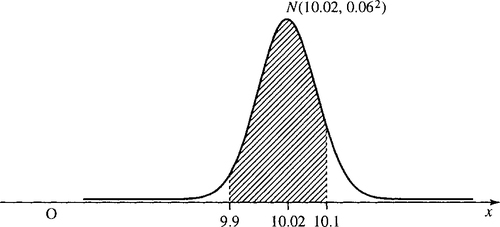
First, convert the x values to z values, by using z = (x – μ) / σ:

So we now want to find the shaded area for z values (which will be the same area as above), shown in Figure 23.27.
In order to use Table 21.3, we need to express the problem in terms of the proportion that lies outside of the tolerance limits, as in Figure 21.28.
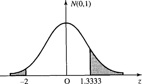

We use the table of the standardized normal distribution to find the proportion less than z = – 2. As the curve is symmetric this will be the same as the proportion greater than z = 2. From the table this gives 0.02275.
The proportion greater than z = 1.33 from the table is 0.09176. Hence, the proportion that lies outside of our limits is
![]()
As the total area is 1, the proportion within the limits is 1 – 0.11451 = 0.88549.
21.11 The exponential distribution
The exponential distribution is also named as the failure rate function, as it can be used to model the rate of failure of components.
Consider a set of 1000 light bulbs, a similar make to those tested in Section 21.1. However, now consider a batch of bulbs at random that have already been in use for some, unknown time. They are, therefore, of mixed ages. On measuring the time of failure we get Table 21.4.
Table 21.4
Time to failure of a sample of light bulbs
| Time of failure (h) | Class mid-point | Frequency | Cumulative frequency | fi xi |
| 0–200 | 100 | 260 | 260 | 26000 |
| 200–400 | 300 | 194 | 454 | 58200 |
| 400–600 | 500 | 154 | 608 | 77000 |
| 600–800 | 700 | 100 | 708 | 70000 |
| 800–1000 | 900 | 80 | 788 | 72000 |
| 1000–1200 | 1100 | 60 | 848 | 66000 |
| 1200–1400 | 1300 | 38 | 886 | 49400 |
| 1400–1600 | 1500 | 33 | 919 | 49500 |
| 1600–1800 | 1700 | 23 | 942 | 39100 |
| 1800–2000 | 1900 | 14 | 956 | 26600 |
| 2000–2200 | 2100 | 12 | 968 | 25200 |
| 2200–2400 | 2300 | 10 | 978 | 23000 |
| 2400–2600 | 2500 | 9 | 987 | 22500 |
| 2600–2800 | 2700 | 13 | 1000 | 33800 |
| 1000 | 638300 |

These data are represented in a histogram given in Figure 21.29, giving the frequencies and relative frequencies, and Figure 21.30, giving the cumulative frequencies and relative cumulative frequencies.


Notice that Figure 21.29 looks like a dying exponential. This is not unreasonable as we might expect failure rates to be something like the problem of radioactive decay of Chapter 8, that is, a dying exponential.
We could think of it in a similar way to a population problem. The proportion that have failed after time t is given by the cumulative distribution function F. The proportion that are still functioning is therefore 1 − F. The increase in the total proportion of failures is given by the failure rate multiplied by the number still functioning, if λ is the failure rate this gives
![]()
This differential equation can be solved to give:
![]()
Using the fact that at time 0 there are no failures then we find A = 1. This gives the cumulative distribution of the exponential distribution as
![]()
where λ is the failure rate, that is, the proportion that will fail in unit time. The probability distribution can be found from the cumulative distribution by differentiating, giving
![]()
Mean and standard deviation of a continuous distribution
We can find the mean and standard deviation of a continuous distribution by using integration to replace the summation over all values. The mean is given by
![]()
where the integration is over all values in the sample space for x. For the exponential distribution this gives
![]()
which can be found by using integration by parts (Chapter 7) to be ![]()
The standard deviation is given by
![]()
where the integration is over all values of x. For the exponential distribution this gives
![]()
Again using integration by parts, we obtain ![]()
So we see that the mean is 1/λ, as is the standard deviation for the exponential distribution.
Comparison of the data with the model
We can now compare a statistical model with the data given in Table 21.4. To do this we calculate the cumulative frequencies for the maximum value in each of the class intervals. The mean of the sample is 638.3. We calculated that the mean of the exponential distribution is given by ![]() the inverse of the failure rate.
the inverse of the failure rate.
and so on, giving the values as in Table 21.5. The model's predictions agree quite well with the data. To find the model predicted frequencies and cumulative frequencies we multiply by the number in the sample, 1000.
Table 21.5
Time to failure of a sample of light bulbs compared with values obtained by modelling with the exponential distribution
| Data | Model predictions | |||||||
| Time of failure (h) | Class mid-point | Frequency | Cumulative frequency | fi xi | F (x) | Probabilities | Cumulative frequency | Frequency |
| 0–200 | 100 | 260 | 260 | 26000 | 0.269 | 0.269 | 269 | 269 |
| 200–400 | 300 | 194 | 454 | 58200 | 0.466 | 0.197 | 466 | 197 |
| 400–600 | 500 | 154 | 608 | 77000 | 0.609 | 0.143 | 609 | 143 |
| 600–800 | 700 | 100 | 708 | 70000 | 0.714 | 0.105 | 714 | 105 |
| 800–1000 | 900 | 80 | 788 | 72000 | 0.791 | 0.077 | 719 | 77 |
| 1000–1200 | 1100 | 60 | 848 | 66000 | 0.847 | 0.056 | 847 | 56 |
| 1200–1400 | 1300 | 38 | 886 | 49400 | 0.888 | 0.041 | 888 | 41 |
| 1400–1600 | 1500 | 33 | 919 | 49500 | 0.918 | 0.03 | 918 | 30 |
| 1600–1800 | 1700 | 23 | 942 | 39100 | 0.940 | 0.022 | 940 | 22 |
| 1800–2000 | 1900 | 14 | 956 | 26600 | 0.956 | 0.016 | 956 | 16 |
| 2000–2200 | 2100 | 12 | 968 | 25200 | 0.968 | 0.012 | 968 | 12 |
| 2200–2400 | 2300 | 10 | 978 | 23000 | 0.977 | 0.009 | 977 | 9 |
| 2400–2600 | 2500 | 9 | 987 | 22500 | 0.983 | 0.006 | 983 | 6 |
| 2600–2800 | 2700 | 13 | 1000 | 33800 | 0.988 | 0.005 | 988 | 5 |
| 638300 | ||||||||

21.12 The binomial distribution
Consider a random system with a sequence of trials, the trials being such that:
1. Each trial has two possible outcomes (e.g. non-defective, defective), which we assign the outcomes of 1 (success) and 0 (failure). This type of trial is called a Bernoulli trial.
2. On each trial p(l)= θ and p(0)= 1 –θ and θ is the same on all trials.
3. The outcome of the n trails are mutually independent.
Pn (r) is the outcome of r successes in n trials and
![]()
where
![]()
Setting α = 1 –θ the probability of r successes in n trials is given by the rth term in the binomial expansion:
Hence, the term binomial distribution.
Example 21.14
In five tosses of a coin find the probability of obtaining three heads.
Solution Assign the outcome of obtaining a head to 1 and tail to 0. Assume that the coin is fair and therefore ![]() The probability of obtaining three heads in five tosses of a coin is given by the binomial probability:
The probability of obtaining three heads in five tosses of a coin is given by the binomial probability:
![]()
Mean and variance of a single trial
The mean of a discrete distribution can be found by using µ = Σxp (x) and the variance is
![]()
where the summation is over the sample space.
We can use these to find the mean and variance of a single trial with only two outcomes, success or failure. The outcome of success has the value 1 and occurs with probability θ and the outcome of failure has the value 0 with probability 1 – θ. Then, the mean is given by 1 × θ + (1 – θ) × 0 = θ.
The variance of a single trial is given by

The standard deviation is the square root of the variance:
![]()
The mean and standard deviation of the binomial distribution
The expressions involving a summation over the entire sample space can be used to find the mean and standard deviation of the binomial distribution but they take a bit of manipulation to find. Instead, we can take a short cut and use the fact that each trial is independent. The mean of the union of n trials is given by the sum of the means of the n trials. Similarly (for independent trials only), the variance of the union of the n trials is given by the sum of the variances.
Therefore, the mean of the binomial distribution for n trials is given by the number of trials × mean for a single trial = nθ. The variance is given by nθ (1 – θ) and therefore the standard deviation is
![]()
Example 21.15
A file of data is stored on a magnetic tape with a parity bit stored with each byte (8 bits) making 9 bits in all. The parity bit is set so that the 9 bits add up to an even number. The parity bit allows errors to be detected, but not corrected. However, if there are two errors in the 9 bits then the errors will go undetected, three errors will be detected, four errors undetected, etc. A very poor magnetic tape was tested for the reproduction of 1024 bits and 16 errors were found. If on one record on the tape there are 4000 groups of 9 bits, estimate how many bytes will have undetected errors.
Solution Call 1 the outcome of a bit being in error and 0 that it is correct. We are given that in 1024 (n) trials there were 16 errors. Taking 16 as the mean over 1024 trials and using
![]()
Errors go undetected if there are 2,4,6, etc. The probability of two errors in 9 bits is given by
![]()
Multiplying by the number of data bytes of 4000 gives approximately 31 undetected errors.
The probability of four errors will obviously be much less.
![]()
This probability is too small to show up only 4000 bytes. As the probability of six or eight errors is even smaller then they can safely be ignored.
The probable number of undetected errors is 31.
21.13 The Poisson distribution
The Poisson distribution is used to model processes where the distribution of the number of incidents occurring in any interval depends only on the length of that interval. Examples of such systems are:
1. incoming telephone calls to an exchange during a busy period;
2. customers arriving at a checkout counter in a supermarket from 4 to 6p.m.;
3. accidents on a busy stretch of the M1;
4. number of misprints in a book.
When modelling situations in a Poisson process we use four assumptions:
1. If A is the event of n incidents in an interval and B the event of m incidents in another non-overlapping interval then A and B are independent, that is, p(A∩B) = p(A)p(B).
2. If A is the event of n incidents in an interval then P(A) depends only on the length of the interval– not on the starting point of the interval.
3. The probability of exactly one incident in a small interval is approximately proportional to the length of that interval, that is, ![]() for small t.
for small t.
4. The probability of more than one incident in a small interval is negligible. Thus, for small t, P2 (t) ≈0 and we can also say that
![]()
It follows that P0(t) + P1(t) ≈ 1 and as by assumption (3), P1(t) ≈ λt we get P0(t) ≈ 1 – λt. We now think about the number of incidents in an interval of time of any given length, (0, t), where t is no longer small. We can divide the interval into pieces of length h, where h is small, and use the assumptions above. We can see that in each small interval of length h there is either no event or a single event. Therefore, each small interval is approximately behaving like a Bernoulli trial. This means that we can approximate the events in the interval (0, t) by using the Binomial distribution for the number of successes r in n trials. The probability of r incidents in n intervals, where the probability of an incident in any one interval is λh, is given by
![]()
Substituting h = t / n gives
![]()
We can reorganize this expression, by taking out of the limit terms not involving n
![]()
We can rewrite the first term inside the limit to give
![]()
Now we notice that the first term inside the limit is made up of the product of r fractional expressions, which each have a term in n on the top and bottom lines. These will all tend to 1 as n tends to ∞. The last term is similar to the limit that we saw in Chapter 7 when calculating the value of e. There, we showed that
![]()
and by a similar argument we could show that
![]()
It, therefore follows that
![]()
The last expression involves a negative power of (1− λt/n), which will tend to 1 as n tends to ∞.
This gives the Poisson distribution as
![]()
This is an expression in both r and t where r is the number of events and t is the length of the time interval being considered. We usually consider the probability of r events in an interval of unit time, which gives the Poisson distribution as
![]()
where λ is the expected number of incidents in unit time.
The mean and variance of the Poisson distribution
The Poisson distribution was introduced by considering the probability of a single event in a small interval of length h as (λh). We then used the binomial distribution, with θ = λh and h = t/n and n tending to ∞, to derive the expression for the Poisson distribution. As the mean of the binomial distribution is nθ it would make sense that the mean of the Poisson distribution is nλh. Using n = t/h we get the mean as λt over an interval of length t and therefore the mean is λ over an interval of unit length.
By a similar argument we know that the variance of the Binomial distribution is nθ(1 – θ). Substituting θ = λh we get the variance as nλh(1 – λh). As n tends to infinity and h to 0 we get the limit λt. Therefore, the variance in unit time is λ.
Example 21.16
The average number of ‘page not found’ errors on a web server is 36 in a 24-h period. Find the probability in a 60-min period that:
(b) there is exactly one error;
(c) There are at most two errors;
(d) there are more than three errors.
Solution Assuming that the above process is a Poisson process, then we have that the average number of errors in 24 h is 36 and therefore the average is 1.5 in 1 h. As the mean is λ, we can now assume that the number of errors in 1 h follows a Poisson distribution with λ = 1.5, giving
![]()
(a) We want to find P(no errors) = Po = ((1.5)0/0!)e−1.5= e−1.5 ≈0.2231.
(b) We want to find P(exactly one error) = P1= (1.5)1 /1!e−1.5 = 1.5e−1.5 ≈0.3347.
(c) p (at most two errors) = Po + P1 + P2= 0.2231 + 0.3347 + (1.5)2/2!e−1.5 = 0.8088.
(d) P(more than three errors) = 1 –P (at most three errors) = 1 – (P0+ P1+ P2+ P3).
Using the result from Part (c) we get
![]()
21.14 Summary
1. The mean of a sample of data can be found by using
![]()
where the summation is over all sample values and n is the number of values in the sample. If the sample is divided into class intervals then
![]()
where xiis a representative value for the class, fiis the class frequency, and the summation is over the all classes.
2. The standard deviation of a sample of data can be found by using
![]()
where the summation is over all sample values, n is the number of values in the sample, and ![]() is the sample mean. If the sample is divided into class intervals then
is the sample mean. If the sample is divided into class intervals then
![]()
where xiis a representative value for the class, fiis the class frequency, ![]() is the sample mean, and the summation is over all classes. The square of the standard deviation is called the variance.
is the sample mean, and the summation is over all classes. The square of the standard deviation is called the variance.
3. The cumulative frequency is found by summing the values of the current class and all previous classes. It is the ‘number so far’.
4. The relative frequency of a class is found by dividing the frequency by the number of values in the data sample – this gives the proportion that fall into that class. The cumulative relative frequency is found by dividing the relative frequency by the number in the sample.
5. In probability theory the set of all possible outcomes of a random experiment is called the sample space. The probability distribution function, for a discrete sample space, is a function of the outcomes that obeys the conditions:
![]()
where xiis any outcome in the sample space and
![]()
where the summation is over all outcomes in the sample space.
6. An event is a subset of the sample space. The probability of an event (if all outcomes are equally likely) is
![]()
7. The addition law of probability is given by P(AU B) = P(A) + P(B) –(A ∩B) for non-disjoint events.
If A∩B =ø this becomes P(A∪B) = P(A)+P(B)for disjoint events.
8. Multiplication law of probabilities: p(A∩B) = p(A) p(B|A) if events A and B are not independent.
9. The definition of independence is that B is independent of A if the probability of B does not depend on A:p(B|A)= p(B) if B is independent of A. In this case the multiplication law becomes p(A∩B) = p(A)p(B), where A and B independent events.
10. Bayes's theorem is
![]()
11. The normal, or Gaussian, distribution is a bell-shaped distribution. Many things, particularly involving error distributions, have a probability distribution that is approximately normal.
12. To calculate probabilities using a normal distribution we use areas of the standard normal distribution in table form, so the variable must be standardized by using the transformation
![]()
where μ is the mean and σ the standard deviation of the distribution.
13. The exponential distribution is used to model times to failure.
14. The probability density function of the exponential distribution is f(t) = λ e−λtand the cumulative density function is given by F = 1– e−λt.
15. The mean and standard deviation of a continuous distribution can be found by
![]()
where the integration is over the sample space. For the exponential distribution these give µ = 1/λ , that is, the mean time to failure is the reciprocal of the failure rate. Also σ = 1/λ.
16. The binomial distribution is a discrete distribution that models repeated trials where the outcome of each trial is either success or failure and each trial is independent of the others. Its probability function is
![]()
where
![]()
and r is the number of successes in n trials.
17. The mean of a discrete distribution is given by µ = Σxp(x) and the variance is σ2= Σ(x −µ)2p(x). mean of the binomial distribution, for n trials, is nθ, the variance is nθ (1 – θ), and the standard deviation ![]()
18. For the Poisson distribution the number of incidents occurring in any interval depends only on the length of that interval. Its probability function is
![]()
where λ is the expected number of incidents in unit time. The mean and the variance are λ.
21.15 Exercises
21.1. An integrated circuit design includes a capacitor of 100 pF (picofarads). After manufacture, 80 samples are tested and the following capacitances found for the nominal 100-pF capacitor (the data are expressed in pF)
Express the data in table form and draw a histogram. Find the mean and standard deviation.
21.2. What is the probability of throwing a number over 4 on one throw of a die?
21.3. What is the probability of throwing a number less than 4 or a 6 on one throw of a die?
21.4. What is the probability of throwing an odd number or a number over 4 on one throw of a die?
21.5. What is the probability of drawing any Heart or a King from a well shuffled pack of cards?
21.6. On two throws of a die, what is the probability of a 6 on the first throw followed by an even number on the second throw?
21.7. Throwing two dice, what is the probability that the sum of the dice is 7?
21.8. What is the probability that the first two cards dealt from a pack will be clubs.
21.9. A component in a communication network has a 1% probability of failure over a 24-h period. To guard against failure an identical component is fitted in parallel with an automatic switching device should the original component fail. If that also has a 1% probability of failure what is the probability that despite this precaution the communication will fail?
21.10. Find the reliability of the system, S, in Figure 21.31. Each component has its reliability marked in the figure. Assume that each of the components is independent of the others.

21.11. A ball is chosen at random out of a bag containing two black balls and three red balls and then a selection is made from the remaining four balls. Assuming all outcomes are equally likely, find the probability that a red ball will be selected:
(b) the second time;
(c) both times.
21.12. A certain brand of compact disc (CD) player has an unreliable integrated circuit (IC), which fails to function on 1% of the models as soon as the player is connected. On 20% of these occasions the light displays fail and the buttons fail to respond, so that it appears exactly the same as if the power connection is faulty. No other component failure causes that symptom. However, 2% of people who buy the CD player fail to fit the plug correctly, in such a way that they also experience a complete loss of power. A customer rings the supplier of the CD player saying that the light displays and buttons are not functioning on the CD. What is the probability that the fault is due to the IC failing as opposed to the poorly fitted plug?
21.13. If a population, which is normally distributed, has mean 6 and standard deviation 2, then find the proportion of values greater than the following:
(b) 10
(c) 12
(d) 7
21.14. If a population, which is normally distributed, has mean 3 and standard deviation 4, find the proportion of values less than the following:
(b) –5
(c) –1
(d) 0
21.15. If a population, which is normally distributed, has mean 10 and standard deviation 3, find the proportion of values that satisfy the following:
(b) x < 12
(c) x > 9
(e) x < 11
(f) 9 < x < 11
(g) 3 < x < 12
21.16. A car battery has a mean life of 4.2 years and a standard deviation of 1.3 years. It is guaranteed for 3 years. Estimate the percentage of batteries that will need replacing under the guarantee.
21.17. A certain component has a failure rate of 0.3 per hour. Assuming an exponential distribution calculate the following:
(a) the probability of failure in a 4-h period;
(b) the probability of failure in a 30-min period;
(c) the probability that a component functions for 1 h and then fails to function in the second hour;
(d) of a group of five components the probability that exactly two fail in an hour.
21.18. A certain town has 50 cash dispenser machines but due to inaccessibility is only visited for repairs once a week after which all the machines are working. The failure rate of the machines is approximately 0.05 per 24 h. A town councillor makes a public complaint in a newspaper that on average at least one in 10 of the machines does not function. Assume an exponential model and calculate the number that are not functioning 1 day, 2 days,. …, 7 days after the day of the visit. Take the mean of these results to assess whether the councillor is correct.
21.19. A bag contains two red balls and eight green balls. A ball is repeatedly chosen at random from the bag, its colour recorded and then replaced. Find the following probabilities:
(a) the first three picked were green;
(b) in a selection of five there were exactly two red balls;
(c) there were no more than three red balls out of the first 10.
21.20. One hundred CDs, each containing 74 min of recording time, were tested for defects. The frequency of defects is given in Table 21.6. Calculate the mean number of defects per 74 min of recording time and choose an appropriate probability model. Using your model copy, complete the two empty columns of the table. Comment on the agreement between the number of incidents and the chosen model frequencies.
Table 21.6
Data for Exercise 21.20
| Number of defects in 74 min of recording time | Number of CDs with r defects | Chosen model probabilities | Chosen model frequencies |
| 0 | 23 | ||
| 1 | 32 | ||
| 2 | 26 | ||
| 3 | 12 | ||
| 4 | 5 | ||
| 5 | 2 | ||
| 6+ | 0 |

21.21. Telephone calls are received at a call centre at a rate of 0.2 per second on average. Calculate the probability that more than 11 calls are received in 1 min.
21.22. Tankers arrive at a dock at a rate of four per day. Assume that the arrivals are a Poisson process and find the following:
(a) the probability that less than five tankers arrive during 1 day;
(b) the probability that there are over five arrivals;
(c) the probability that there is exactly five arrivals;
(d) The probability that there are between two and five inclusive, arrivals.