
The exponential function
8.1 Introduction
In Example 2.11, we looked at an acoustical absorption problem. We found that after a single note on a trombone had been played, the sound intensity decayed according to the expression I = 10−11t. This is a dying exponential function. Many other physical situations involve decay or growth in an exponential fashion; for instance, population growth or the decay of charge on a discharging capacitor. The functions y = at, where a can be any positive number, are called exponential functions. In this chapter, we shall look at how they describe this particular type of growth or decay, when the growth or decay is proportional to the current size of the ‘population’, y. This situation can be described by a differential equation of the form dy/dt = ky. The special case where k = 1, giving the equation dy/dt = y, leads us to define the number e ≈ 2.7182818 and the function y = et, which is called the exponential function. The inverse function is y = loge(t), which is also refered to as y = In(t) and called the natural or N apierian logarithm.
The function y = et is neither even nor odd; however, it is possible to split any real function into an even part and an odd part and in this case we find that this gives the hyperbolic functions. These hyperbolic functions have properties that are surprisingly similar to the properties of the trigonometric functions and hence have similar names, cosh(t), sinh(t) (the hyperbolic sine and hyperbolic cosine) from which we can define also tanh(t), the hyperbolic tangent. We also look at differentiation and integration problems involving the exponential and hyperbolic functions.
8.2 Exponential growth and decay
Supposing, following some deed of heroism, the police offered you the choice of the following rewards:
(a) Tomorrow you receive 1 c and the following day 2 c and after that 4 c, then 8 c and each day the amount doubles for the next month.
(b) Tomorrow you receive €2, the following day €4 and the day after €6, then €8 so that each day you receive €2 more than the day before. Again you receive payments on every day for the next month.
If, although not motivated by personal greed, you wish to receive the highest possible reward (in order, presumably, to donate the amount to charity), which reward should you accept? Option (b) superficially appears to be the best because at least it starts off with enough money to buy a small sandwich. However, a closer look reveals the that if you choose option (a), on the last day (assuming there are 31 days in the month) you receive in excess of € 10 000 000 with the total reward exceeding €20 million. However, option (b) only reaps €62 on the final day with a total award of only €992.
Both options are examples of growth. Option (b) gives a constant growth rate of €2. If yn is the amount received on day n, the way that this grows could be expressed by yn + 1 = yn + 2. This is expressing the fact that the amount received on day n + 1 is €2 more than the amount received on day n. This also means that the change each day in the amount received is 2, which can be expressed as Δyn = 2, where Δyn = yn+l – yn and represents the change in y from day n to day n + 1.
Option (a) is an example of exponential growth (or geometric growth). The amount received each day is proportional to the amount received the day before, in this case twice as much. yn can be expressed by yn + 1 = 2 yn. The change in y is equal to the value of y itself, Δyn = yn.
Because of the nature of exponential growth it is unlikely that you would be given such an attractive award as option (a) represents. However, exponential growth is not beyond the reach of the everyday person as savings accounts offer this opportunity. Unfortunately, the amount you receive does not increase as quickly as doubling each day but it is based on how much you have already in the bank; hence, it is exponential. Supposing you opened an account that paid an annual interest of 6% and the annual rate of inflation was 3%, then the real rate of growth is approximately 3% per annum. If yn is the value of the amount you have in the bank after n years then yn+l = 1.03yn. We can also express this by saying that the interest received each year, that is, the change in yn, Δyn, is 3% of yn, that is, Δyn = 0.03yn, where Δyn = yn+l – yn. If the rate of interest remains constant then if you deposit €1 tomorrow then your descendents, in only 500 years time, will receive an amount worth over €2.5 million in real terms.
The models of growth that we have discussed so far give examples of recurrence relations, also called difference equations. Their solutions are not difficult to find. For instance, if yn + 1 = 2 yn and we know that on day 1 we received 1 c, that is, y1 = 0.01 then we can substitute n = 1,2,3, … (as we did in Section 1.4) to find values of the function giving
0.01,0.02,0.04,0.08,0.016,0.032,…
![]()
Clearly, there is a power of 2 involved in the expression for yn, so we can guess that y = 0.01 (2n−1). By checking a few values of n we can confirm that this is indeed the amount received each day. When we deposit €1 in the bank at a real rate of growth of 3% we get the recurrence relation yn + 1 = 1.03 yn, where yn is the current day value of the amount in the savings account after n years. Substituting a few values beginning with y0 = 1 (the amount we initially deposit) we then get 1,1.03,1.06,1.09,1.13,1.16,1.19, … (to the nearest cent). Each time we multiply the amount by 1.03, there must be a power of 1.03 in the solution for y. We can guess the solution as yn = (1.03)n. By checking a few values of n we can confirm that this is, in fact, the amount in the bank after n years.
The models we have looked at so far are discrete models. In the case of the money in the bank the increase occurs at the end of each year. However, if we consider population growth, for instance, then it is not possible to say that the population grows at the end of a certain period, the growth could happen at any moment of time. In this case, providing the population is large enough, it is easier to model the situation continuously, using a differential equation. Such models take the form of dy/dt = ky. dy/dt is the rate of growth, if k is positive, or the rate of decay, if k is negative. The equation states that the rate of growth or decay of a population of size y is proportional to the size of the population.
Example 8.1
A malfunctioning fridge maintains a temperature of 6°C which allows a population of bacteria to reproduce such that, on average, each bacteria divides every 20 min. Assuming no bacteria die in the time under consideration find a differential equation to describe the population growth.
Solution If the population at time t is given by p then the rate of change of the population is dp/dt. The increase in the population is such that it approximately doubles every 20 min, that is, it increases by p in 20 × 60 s. That gives a rate of increase as p/(20 × 60) per second. Hence, the differential equation describing the population is
dpdt=p1200.

Example 8.2
A capacitor, in an RC circuit, has been charged to a charge of Q0. The voltage source has been removed and the circuit closed as in Figure 8.1. Find a differential equation that describes the rate of discharge of the capacitor if C = 0.001 μF and R = 10MΩ.

Solution The voltage across a capacitor is given by Q/C where C is the capacitance and Q is the charge on the capacitor. The voltage across the resistor is given by Ohm's Law as IR. From Kirchoff's voltage law, the sum of the voltage drops in the circuit must be 0; therefore, as the circuit is closed, we get voltage across the resistor + voltage across the capacitor = 0:
⇒IR+QC=0.
![]()
By definition, the current is the rate of change of charge with respect to time, that is I = d Q/dt giving the differential equation
RdQdt+QC=0.
We can rearrange this equation as
RdQdt=−QC⇔dQdt=−QRC.

We can see that this is an equation for exponential decay. The rate of change of the charge on the capacitor is proportional to the remaining charge at any point in time with a constant of proportionality given by 1/RC. In this case as R = 10MΩ and C = 0.001 μF, we get
dQdt=−100Q.
Example 8.3
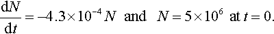
Radioactivity is the emission of α- or, β-particles and γ-rays due to the disintegration of the nuclei of atoms. The rate of disintegration is proportional to the number of atoms at any point in time and the constant of proportionality is called the radioactivity decay constant. The radioactive decay constant for Radium B is approximately 4.3 × 10⁻⁴ s−1. Give a differential equation that describes the decay of the number of particles N in a piece of Radium B.
Solution If the number of particles at time t is N, then the rate of change is dN/dt. The decay is proportional to the number of atoms, and we are given that the constant of proportionality is 4.3 × 10⁻⁴ s−1 so that we have
dNdt=−4.3×10⁻⁴N
![]()
as the equation which describes the decay.
Example 8.4
An object is heated so that its temperature is 400 K and the temperature of its surroundings is 300 K, and then it is left to cool. Newton's law of cooling states that the rate of heat loss is proportional to the excess temperature over the surroundings. Furthermore, if m is the mass of the object and c is its specific heat capacity then the rate of change of heat is proportional to the rate of fall of temperature of the body, and is given by
dQdt=−mcdϕdt
![]()
where Q is the heat in the body and ϕ is its temperature. Find a differential equation for the temperature that describes the way the body cools.
Solution Newton's law of cooling gives
dQdt=A(ϕ−ϕs)
![]()
where A is some constant of proportionality, Q is the heat in the body, ϕ is its temperature, and ϕs is the temperature of its surroundings. As we also know that
dQdt=−mcdϕdt

this can be substituted in our first equation giving:
−mcdϕdt=A(ϕ−ϕs)⇔dϕdt=−Amc(ϕ−ϕs)

A/(mc) can be replaced by a constant k, giving
dϕdt=−k(ϕ−ϕs).
In this case, the temperature of the surroundings is known to be 300 K, so the equation describing the rate of change of temperature is
dϕdt=−k(ϕ−300).

We have established that there are a number of important physical situations that can be described by the equation dy/dt = ky. The rate of change of y is proportional to its value. We would like to solve this equation, that is, find y explicitly as a function of t. In Chapter 7, we solved simple differential equations such as dy / dt = 3t by integrating both sides with respect to t, for example,
dydt=3t⇔y=∫3t?dt⇔y=3t22+C.
However, we cannot solve the equation dy/dt = ky in this way because the right-hand side is a function of y not of t. If we integrate both sides with respect to t we get
dydt=ky⇔y=∫ky?dt.
Although this is true we are no nearer solving for y as we need to know y as a function of t in order to find ∫ ky dt.
When we solved equations in Chapter 3 of the Background Mathematics notes available on the companion website for this book, we said that one method was to guess a solution and substitute that value for the unknown into the equation to see if it gave a true statement. This would be a very long method to use unless we are able to make an informed guess. We can use this method with this differential equation as we know from our experience with problems involving discrete growth that a solution should involve an exponential function of the form y = at. The main problem is to find the value of a, which will go with any particular equation. To do this we begin by looking for an exponential function that would solve the equation d y / dt = y, that is, we want to find the function whose derivative is equal to itself.
8.3 The exponential function y = et
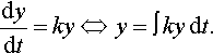
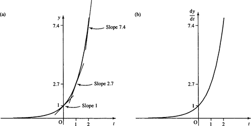
Figures 8.2(a) and 8.3(a) give graphs of y = 2t and y = 3t, which are two exponential functions. We can sketch their derivative functions by drawing tangents to the graph and measuring the gradient of the tangent at various different points. The derivative functions are pictured in Figure 8.2(b), dy/dt where y = 2t, and in Figure 8.3(b), dy/dt where y = 3t.

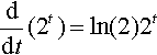
We can see that for these exponential functions the derivative has the same shape as the original function but has been scaled in the y-direction, that is, multiplied by a constant, k, so that dy/dt = ky as we expected:
ddt(2t)=(C)(2t)????and????ddt(3t)=(D)(3t)
where C and D are constants. We can see from the graphs that C < 1 and D > 1. Thus, the derivative of 2t gives a squashed version of the original graph and the derivative of 3tgives a stretched version of the original graph.
It would seem reasonable that there would be a number somewhere between 2 and 3 that we can call e, which has the property that the derivative of et is exactly the same as the original graph. That is,
ddt(et)=et.
Finding the value of e
There are various methods for finding the value of e and a graphical investigation into finding e to one decimal place is given in the projects and investigations available on the companion website for this book. An alternative, numerical, method is to look at the gradient of the chord for the function y = et at t = 0:
δyδt=f(t+δt)−δtδt=et+δt−etδt
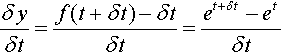
At t = 0 all functions y = at have value 1 so that the gradient of the chord at t = 0 is
δyδt=eδt−1δt
![]()
We defined e as the number for which ddt(et) = etso that at the point t = 0 the gradient of the tangent is given by dy/dt = 1. For small δt the gradient of the tangent is approximately equal to the gradient of the chord
dydt≈δyδt
![]()
and therefore
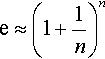
1≈eδt−1δt

Rearranging this equation gives e ≈ (1+δt)1/δt![]() for small δt. Replacing δt by l/n, with n large, gives
for small δt. Replacing δt by l/n, with n large, gives
e≈(1+1n)n
![]()
for large n.
Let n tend to infinity and this gives the well-known limit
e=limn→∞(1+1n)n.

We can use the expression
e≈(1+1n)n
for large n to calculate e on a calculator. This is done in Table 8.1 to five decimal places.
Table 8.1
Estimating e using (1 ± 1/ n)n gives e = 2.71828 to five decimal places
| n | (1 + (1/n))n to five decimal places |
| 1000 | 2.71692 |
| 10 000 | 2.71815 |
| 100 000 | 2.71827 |
| 1 000 000 | 2.71828 |
| 10 000 000 | 2.71828 |
We have shown that e = 2.71828 to five decimal places. e is an irrational number which means that it cannot be written exactly as a fraction (or as a decimal). The function et is often referred to as exp(t). etand its derivative are shown in Figure 8.4.
By definition of the logarithm (as given in Chapter 4 of the Background Mathematics notes available on the companion website for this book), we know that the inverse function to et is loge (t) (log, base e, of t). This is often represented by the short hand of In (t) and called the natural or Napierian logarithm.
We are now able to solve the differential equation dy/dt = y as we know that one solution is y = et because the derivative of y = et is et. When we discussed differential equations in Chapter 7, we noticed that there was an arbitrary constant that was involved in the solution of a differential equation. In this case the constant represents the initial size of the population, or the initial charge or the initial number of atoms or the initial temperature. The general solution to dy/dt = y is y = y0et where y0 is the value of y at time t = 0. We can show that this is, in fact, the general solution by substituting into the differential equation.
Example 8.5
(a) Show that any function of the form y = y0et, where y0 is a constant, is a solution to the equation
dydt=y

(b) Show that in the function y = yoet, y = y0 when t = 0.
Solution
(a) To show that y = y0etare solutions, we first differentiate
ddt(y0et)=y0et
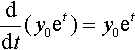
(as y0 is a constant and d (et)/dt = et).
Substitute for d y/dt and for y into the differential equation and we get y0et= y0et, which is a true statement for all t. Hence the solutions to dy/dt = y are y = y0et.
(b) Substitute t = 0 in the function y = y0et and we get y = y0eo. As any number raised to the power of 0 is 1, we have y = y0. Hence y0 is the value of y at t = 0.
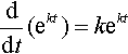
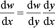
Using the function of a function rule we can find the derivative of ekt, where k is some constant, and show that this function can be used to solve differential equations of the form dy/dt = ky.
The derivative of ekt
To find the derivative of y = ektwhere k is a constant substitute u = kt so that y = eu
dudt=k????and????dydu=eu
![]()
therefore, using the chain rule,
dydt=dudtdydu=k?eu=k?ekt
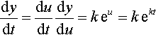
(resubstituting u = kt). Therefore,
ddt(ekt)=k?ekt
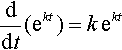
Notice that if we substitute y for ekt into d(ekt)/dt = kekt we get dy/dt = ky, which was the differential equation we set out to solve for our growth or decay problems.
This tells us that one solution to the equation dy/dt = ky is y = ekt. The general solution must involve a constant, so we try y = y0ektwhere y0 is the initial size of the population, or initial temperature, etc.
Example 8.6
(a) Show that any function of the form y = y0ekt, where y0 is a constant, is a solution to the equation
dydt=ky

(b) Show that in the function y = y0ekt, y = y0 when t = 0.
Solution
(a) To show that y = y0ekt are solutions we first differentiate:
ddt(y0ekt)=y0kekt

as y0 is a constant and d(ekt)/dt = kekt. Substitute for dy/dt and for y into the differential equation and we get
y0kekt= ky0ektwhich is a true statement for all values of t. Hence the solutions to dy /dt = ky are y = y0ekt.
(b) Substitute t = 0 in the function y = y0etand we get y = y0e0. As any number raised to the power of 0 is 1, we have y = y0. Hence, y0 is the value of y at t = 0.
Example 8.7
Solve the differential equation given in Example 8.2, describing the discharge of a capacitor in a closed RC circuit with R = 10MΩ and C = 0.001 μF:
dQdt=−100Q

and find a particular solution given that at t = 0 the voltage drop against the capacitor was 1000 V.
Solution We have discovered that the solution to a differential equation of the form dy/dt = kt is given by y = y0ektwhere y0 is the initial value of y.
Comparing dy/dt = ky with dQ/dt = −100Q, and replacing y by Q and k by −100, we get the solution
Q=Q0e−100t
![]()
To find the value of Q0 we need to find the value of Q when t = 0. We are told that the initial value of the voltage across the capacitor was 1000 V and we know that the voltage drop across a capacitor is Q/C. Therefore, we have
Q00.001×10−6=1000⇔Q0=1000×0.001×10−6⇔Q0=10−6C.

Therefore, the equation that describes the charge as the capacitor discharges is Q = 10–6e−100t C at time t s.
The derivative of at
The derivative of y = 2t can now be found by observing that 2 = e (In(2)). Therefore, y = 2t = (eIn(2))t = eIn(2)t. This is of the form ektwith
k = In(2). As
ddt(ekt)=kekt
then
ddt(eln(2)t)=ln(2)etln(2)
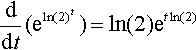
Using again the fact that eIn(2)t = (eIn(2))t = 2t we get
ddt(2t)=ddt(eln(2)t)=ln(2)eln(2)t=ln(2)2t
![]()
that is
ddt(2t)=ln(2)2t
Compare this result to that which we found by sketching the derivative of y = 2t in Figure 8.2(b). We said that the derivative graph was a squashed version of the original graph. This result tells us that the scaling factor is In(2) ≈ 0.693, which confirms our observation that the scaling factor, C < 1.
Using the same argument for any exponential function y = at we find that dy /dt = In(a)at.
In finding these results we have used the fact that an exponential function, to whatever base, a, can be written as ektwhere k = ln(a).
The derivative of y = ln(X)
y = ln(x) is the inverse function of f(x) = ex, and therefore we can find the derivative in a manner similar to that used to find the derivatives of the inverse trigonometric functions in Chapter 5.
y = ln(x) where x > 0
⇔ ey=eln(x)(take?the?exponentiol?of?both?sides)
![]()
⇔ ey=x(as?exp?is?the?inverse?function?to,?eln(x)=x)
![]()
We wish to differentiate both sides with respect to x but the left-hand side is a function of y, so we use the chain rule, setting w = ey, thus, equation ey= x becomes w = x and dw/dy = ey.
Differentiating both sides of w = x with respect to x gives dw/dx = 1, where
dwdx=dwdydydx
from the chain rule. So
eydydx=1

and resubstituting x = eywe get
xdydx=1⇔dydx=1x
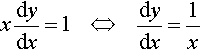
(we can divide by x as x > 0). Hence,
ddx(lnx)=1x.

The derivative of the log, of whatever the base, can be found using the change of base rule for logarithms as given in Chapter 4 of the Background Mathematics notes available on the companion website for this book. We can write
loga(x)=ln(x)ln(a).

Therefore
ddx(loga(x))=ddx(ln(x)ln(a))=1ln(a)x.

8.4 The hyperbolic functions
Any function defined for both positive and negative values of x can be written as the sum of an even and odd function. That is, for any function y = f(x) we can write
f(x)=fe(x)+fo(x)
![]()
where
fe(x)=f(x)+f(−x)2

and
fo(x)=f(x)−f(−x)2.
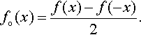
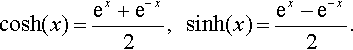
The even and odd parts of the function ex are given the names of hyperbolic cosine and hyperbolic sine. The names of the functions are usually shortened to cosh(x) (read as ‘cosh of x’) and sinh(x) (read as ‘shine of x’).
ex = cosh(x) + sinh (x)
and
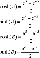
cosh(x)=ex+e−x2,????sinh(x)=ex−e−x2.
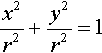
They are called the hyperbolic sine and cosine because they bear the same sort of relationship to the hyperbola as the sine and cosine do to the circle. When we introduced the trigonometric functions in Chapter 5 we used a rotating rod of length r. The horizontal and vertical positions of the tip of the rod as it travels around the circle defines the cosine and sine function, respectively. A point (x, y) on the circle can be defined using x = r cos (α), y = r sin (α). These are called parametric equations for the circle and α is the parameter. If the parameter is eliminated then we get the equation of the circle
x2r2+y2r2=1
(shown in Figure 8.4(a)). Any point on a hyperbola can similarly be defined in terms of a parameter, α, and thus we get x = a cosh(α) and y = b sinh(α).
If the parameter is eliminated from the equations we get the equation for the hyperbola as
x2a2−y2b2=1
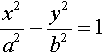
Figure 8.5(b) shows the graph of the hyperbola.
The function y = tanh (x) is defined, similarly to the tan (x), as
tanh(x)=sinh(x)cosh(x)

and the reciprocal of these three main functions may be defined as
cosech(x)=1sinh(x)?????(the?hyperbolic?cosecant)sech(x)=1cosh(x)?????(the?hyperbolic?secant)coth(x)=1tanh(x)?????(the?hyperbolic?secant)

The graphs of cosh(x), sinh (x), and tanh (x) are shown in Figure 8.6.

Hyperbolic identities
The hyperbolic identities are similar to those for trigonometric functions. A list of the more important ones is given in Table 8.2.
Table 8.2
Summary of important hyperbolic identities
cosh(x) = (ex + e-x)/2
sinh(x) = (ex — e-x)/2
tanh(x) = sinh(x)/ cosh(x) = (ex — e-x)/(ex + e-x)
cosh(x) + sinh(x) = ex
cosh(x) — sinh(x) = e-x
cosh(A ± B) = cosh(A) cosh(B) ± sinh(A) sinh(B)
sinh(A ± B) = sinh(A) cosh(B) ± cosh(A) sinh(B)
tanh(A ± B) = (tanh(A) ± tanh(B))/(1 ± tanh(A) tanh(B))
Example 8.8
Show that cosh(A + B) = cosh(A) cosh(B) + sinh(A) sinh(B).
Solution Substitute
cosh(A)=eA+e−A2sinh(A)=eA−e−A2cosh(B)=eB+e−B2sinh(B)=eB+e−B2
into the right-hand side of the expression
cosh(A) cosh(B) + sinh(A) sinh(B)
=(eA+e−A)2(eB+e−B)2(eA−e−A)2(eB−e−B)2.

Multiplying out the brackets gives
14(eA+B+eA−B+e−A+B+e−(A+B)+(eA+B−eA−B−e−A+B+e−(A+B))).
![]()
Simplifying then gives
14(2eA+B+2e−(A+B))=12(eA+B+e−(A+B))
![]()
which is the definition of cosh(A + B).
We have shown that the right-hand side of the expression is equal to the left-hand side, and therefore
cosh(A + B) = cosh(A) cosh(B) + sinh(A) sinh(B).
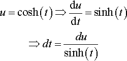
Inverse hyperbolic functions
The graphs of the inverse hyperbolic functions sinh −1 (x), cosh −1 (x), and tanh−1(x) are given in Figure 8.7.
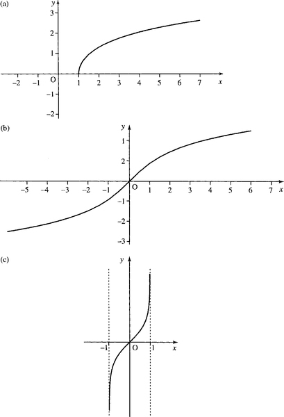
As cosh(x) is not a one-to-one function, it has no true inverse. However, if we limit x to zero or positive values only then cosh −1(x) is indeed the inverse function and cosh −1 (cosh(x)) = x. The sinh −1 (x) function is defined for all values of x, but cosh −1 (x) is defined for x ≥ 1 only and tanh−1(x) is defined for −1 < x < 1.
As the hyperbolic functions are defined in terms of the exponential function we might suspect that the inverse would be defined in terms of the logarithm. The logarithmic equivalences are
sinh−1(x)=ln(x+√x2+1)????for?all?xcosh−1(x)=ln(x+√x2−1)????x≥1tanh−1(x)=12ln(1+x1−x)????−1<x<1

Example 8.9
Show that sinh−1(x)=ln(x+√x2+1)![]() using the definitions
using the definitions
y=sinh−1(x)????⇔????sinh(y)=x
![]()
and
sinh(y)=ey−e−y2

y=sinh−1(x)????⇔????sinh(y)=x
![]()
Using
sinh(y)=ey−e−y2
to substitute on the left-hand side, we get
ey−e−y2=x?????⇔?????ey−e−y=2x????(multiplying?by?2)?????⇔?????e2y−1=2xey????(multiplying?by?ey?and?using?properties?of???????????????????????????????????????????????????????power?to?write?ey⋅ey=e2y)?????⇔?????e2y−2xey−1=0?????(subtracting?2xey?from?both?sides)

This is now a quadratic equation in ey
(ey)2-2xey-1=0.
![]()
Using the formula for solving a quadratic equation, where a = 1, b = −2x, c = −1 gives
ey=2x±√4x2+42.
![]()
Dividing the top and bottom lines by 2 gives
ey=x±√x2+1.
![]()
Taking In of both sides and using In (ey) = y (In is the inverse function of exp) we get
y=ln(x±√x2+1).
![]()
We discount the negative sign inside the logarithm, as this would lead to a negative values, for which the logarithm is not defined. So finally
sinh−1(x)=ln(x+√x2+1).
![]()
Calculations
The hyperbolic and inverse hyperbolic functions are often not given in a calculator. To calculate a hyperbolic function then use the definitions
cosh(x)=ex+e−x2sinh(x)=ex−e−x2tanh(x)=sinh(x)cosh(x)=ex−e−xex+e−x

To calculate the inverse hyperbolic functions use their logarithmic equivalences.
Example 8.10
Calculate the following, and where possible use the appropriate inverse function to check your result:
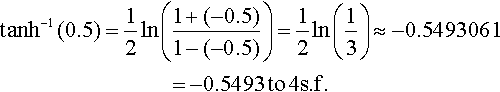
(b) tanh−l (−0.5)
(c) cosh(−1)
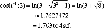
(d) cosh−l(3)
(e) cosh−l(0)
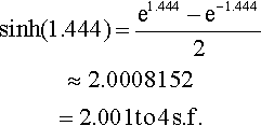
Solution From the definition
sinh(1.444)=e1.444−e−1.4442≈2.0008152=2.001?to?4?s.f.
Check: Use the inverse function of the sinh, that is, find sinh−1 (2.0008152). From the logarithmic equivalence
sinh−1(2.0008152)=ln(2.0008152)+√(2.0008152)2+1=1.444

As this is the original number input into the sinh function we have found sinh−1 (sinh(1.444)) = 1.444, which confirms the accuracy of our calculation.
(b) To calculate tanh −1 (−0.5) use the logarithmic equivalence giving
tanh−1(0.5)=12ln(1+(−0.5)1−(−0.5))=12ln(13)≈−0.5493061=−0.5493?to?4s.f.
Check: Use the inverse function of tanh −1, that is, find
tanh(−0.5493061)=e−0.5493061−e0.5493061e−0.5493061+e0.5493061≈−0.5

This is the original number input to the tanh −1 function and this confirms the accuracy of our calculation.
(c)
cosh(−1)=e−1+e12≈1.5430806=1.543?to?4?s.f.

Check: Use the inverse function of cosh, that is, cosh −1 :
cosh−1(1.5430806)=ln(1.5430806+√1.54308062−1≈1)
![]()
This is not the number that we first started with, which was −1. However, we know that cosh−1(x) is only a true inverse of cosh(x) if the domain of cosh(x) is limited to positive values and zero. We did not expect the inverse to ‘work’ in this case where we started with a negative value.
(d) To calculate cosh−1 (3), use
cosh−1(3)=ln(3+√32−1)=ln(3+√8)≈1.7627472=1.763?to?4?s.f.
Check: The inverse function to cosh −1 is cosh, so we find
cosh(1.7627472)=e1.7627472+e−1.76274722≈3
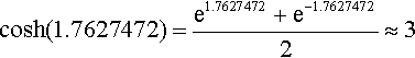
This confirms the accuracy of our calculation as we have shown cosh(cosh −1 (3)) = 3.
(e) Using the logarithmic definition of cosh −1 leads to an attempt to take the square root of a negative number. This confirms that cosh −1 (0) is not defined in ![]() .
.
Derivatives
Derivatives of the hyperbolic functions can be found by reverting to their definitions in terms of the exponential function.
Example 8.11
Show thatddx(sinh(x))=cosh(x)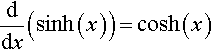
Solution As
sinh(x)=ex−e−x2
![]()
then
ddx(sinh(x))=ddx(ex−e−x2)=ex−(−1)e−x2=ex+e−x2=cosh(x).

Therefore
ddx(sinh(x))=cosh(x).

In a way similar to Example 8.6, we can find
ddx(cosh(x))=sinh(x).

and
ddx(tanh(x))=sech2(x).

The derivatives of the inverse hyperbolic functions can be found using the same method as given for the derivatives of the inverse trigonometric functions (in Chapter 5) and give
ddx(sinh(x))=1√1+x2ddx(cosh−1(x))=1√x2−1ddx(tanh−1(x))=11−x2.

8.5 More differentiation and integration
We are now able to add the functions y = ex and y = ln(x), y = ax, y = log, (x), and the hyperbolic and inverse hyperbolic functions to the list of functions (Table 8.3). By swapping the columns and rearranging some of the terms in a more convenient fashion, and adding the constant of integration, we get a list of integrals (Table 8.4).
Table 8.3
The derivatives of some simple functions
| f (x) | f'(x) |
| C | 0 |
| xn | nxn−1 |
| cos(x) | − sin(x) |
| sin(x) | cos(x) |
| tan(x) | sec2(x) |
| sin−1(x) | 1/√1−x2 |
| cos−1(x) | −1/√1−x2 |
| tan−1(x) | 1/(1+x2) |
| ex | ex |
| ax | (ln(a)ax) |
| ln(x) | 1/x |
| loga(x) | 1/(ln(a)x) |
| cosh(x) | sinh(x) |
| sinh(x) | cosh(x) |
| tanh(x) | sech2(x) |
| sinh−1(x) | 1/√(1+x2) |
| cosh−1(x) | 1/√x2−1 |
| tanh−1(x) | 1/(1−x2) |
Table 8.4
Some standard integrals
| f(x) | ∫ f(x)dxf(x) |
| 1 | x + C |
| xn (n ± —1) | (xn+1)/(n + 1) + C |
| sin(x) | − cos(x) + C |
| cos(x) | sin(x) + C |
| sec2 (x) | tan(x) + C |
| 1/√1−x2 | sin −1 (X) + C |
| −1/√1−x2 | cos−1 (X) + C |
| 1/(1 + x2) | tan−1(x) + C |
| ex | ex + C |
| ax | ax/ In(a)) + C |
| 1/x | In(x) + C |
| cosh(x) | sinh(x) + C |
| sinh(x) | cosh(x) + C |
| sech2(x) | tanh(x) + C |
| 1/√1+x2 | sinh−1(x) + C |
| 1/√x2−1 | cosh−1 (x) + C |
| 1/(1−x2) | tanh−1 (x) + C |
The methods of differentiation and integration of combined functions, discussed in Chapters 12 and 13, can equally be applied to exponential and logarithmic functions.
Example 8.12
Find derivatives of the following:
(a)?y=e−2t2+3????(b)?x=e−tcos(3t)????(c)y=sinh(x)x??x≠0.
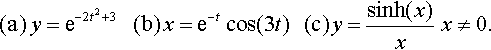
Solution
(a) To differentiate y = e−2t2+3using the function of a function rule think of this as y = e()(‘y = e to the bracket’).
Now differentiate y with respect to () and multiply by the derivative of () with respect to t. That is, use
dydt=dyd()d()dt

where () represents the expression in the bracket
dydt=e−2t2+3ddt(−2t2+3)=e−2t2+3(−4t)=−4te−2t2+3.

(b) To find the derivative of x = e−t cos (3t), write x = uv so that u = e−t and v = cos(3t); then,
dudt=−e−t?????dυdt=−3sin(3t)

where we have used the chain rule to find both these derivatives. Now use the product rule
dxdt=udυdt+υdudt
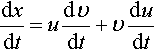
dxdt=−e−tcos(3t)−e−t3sin(3t)=−e−tcos(3t)−3e−tsin(3t).

(c) To find the derivative of
y=sinh(x)x
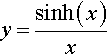
we use the formula for the quotient of two functions where y = u/v, u = sinh (x), v = x, and
dydx=ν(du/dx)−u(dν/dx)ν2

Hence, we get
ddx(sinh(x)x)=xcosh(x)−sinh(x)⋅1x2=x?cosh(x)−sinh(x)x2.

Example 8.13
Find the following integrals:
∫xex2+2dx
![]()
(b)
∫sinh(t)?cosh2(t)?dt
![]()
(c)
∫xex?dx
![]()
(d)
∫21ln(x)dx

(e)
∫(3x2+2xx3+x2+2)dx

Solution
(a) ∫xex2+2dx![]() . Here, we have a function of a function e(x2+2) multiplied by a term that is something like the derivative of the term in the bracket.
. Here, we have a function of a function e(x2+2) multiplied by a term that is something like the derivative of the term in the bracket.
Try a substitution, u = x2+ 2
⇒dudx=2x⇒dx=du2x
![]()
then
∫xex2+2dx=∫xeudu2x=∫12eudu=12eu+C

resubstituting u = x2 + 2 gives
∫xex2+2dx=12ex2+2+C
![]()
(b) To find ∫ sinh(t) cosh2(t) dt we remember that cosh2(t) = (cosh(t))2, so
∫sinh(t)cosh2(t)dt=∫sinh(t)(cosh(t))2dt
![]()
sinh(t) is the derivative of the function in the bracket, cosh(t), so a substitution, u = cosh(t), should work:
u=cosh(t)⇒dudt=sinh(t)⇒dt=dusinh(t)
∫sinh(t)cosh2(t)dt=∫sinh(t)u2dusinh(t)=∫u2du=u3+C

resubstituting u = cosh(t) gives
∫sinh(t)?cosh2(t)dt=cosh3(t)3+C

(c) ∫ xexdx. Use integration by parts
∫u?dν=uν−∫νdu
![]()
and choose u = x and dv = exdx giving
dudx=1andν∫exdx=ex
Then
∫xexdx=xex−∫exdx=xex−ex+C

(d) ∫21ln(x)dx . Write ln(x) = 1 ln (x) and use integration by parts with
u=ln(x)anddν=1?dx
![]()
⇒du=dxxν=∫1?dx=x

∫21ln(x)dx=[x?ln(x)]21−∫21x12dx=2ln(2)−1ln(1)−∫211dx=2ln(2)−[x]21=2ln(2)−(2−1)≈0.3863?to?4s.f.

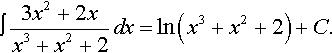
(e) We rewrite
∫3x2+2xx3+x2+2dx=∫(3x2+2x)(x3+x2+2)−1dx.

Notice that there are two brackets. To decide what to substitute we notice that
ddx(x3+x2+2)=3x2+2x.
so it should work to substitute u=x3+x2+2![]()
⇒ddx=3x2+2x⇒dx=dx3x2+2x.
![]()
The integral becomes
∫(3x2+2x)u−1du3x2+2x∫duu=ln(u)+C.

Resubstituting for u gives
∫3x2+2xx3+x2+2dx=ln(x3+x2+2)+C.
Integration using partial fractions
The fact that expressions like 1/ (3x + 2) can be integrated using a substitution which results in an integral of the form:
∫1udu=ln(u)+C
![]()
is exploited when we perform the integration of fractional expressions like
2x−1(x−3)(x+1).

We first rewrite the function to be integrated using partial fractions.
Example 8.14
Find

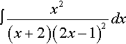
(b) ∫x2(x+2)(2x−1)2dx.![]()
Solution
Rewrite the expression using partial fractions. We need to find A and B so that:
2x−1(x−3)(x+1)=A(x−3)+Bx+1
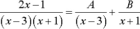
where this should be true for all values of x. Multiplying by (x – 3)(x + 1) gives 2x – 1 = A(x + 1) + B(x – 3). This is an identity, so we can substitute values for x: substitute x = −1 giving – 3 = B( −4) ⇔ B = 3/4 substitute x = 3 giving 5 = A(4) ⇔ A = 5/4
Hence,
2x−1(x−3)(x+1)=54(x−3)+34(x+1).
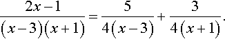
So
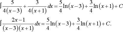
∫2x−1(x−3)(x+1)dx=∫54(x−3)+34(x+1)dx.

As (x – 3) and (x + 1) are linear functions of x, we can find each part of this integral using substitutions of u = x – 3 and u = x + 1:
∫54(x−3)+34(x+1)dx=54ln(x−3)+34ln(x+1)+C∫2x−1(x−3)(x+1)dx=54ln(x−3)+34ln(x+1)+C.
Check:
ddx(54ln(x−3)+34ln(x+1)+C)=54(x−3)+34(x+1)

writing this over a common denominator gives
ddx(54ln(x−3)+34ln(x+1)+C)=5(x+1)+3(x−3)4(x−3)(x+1)=5x+5+3x−94(x−3)(x+1)=8x-44(x−3)(x+1)=2x−1(x−3)(x+1)

Again, we can use partial fractions. Because of the repeated factor in the denominator we use both a linear and a squared term in that factor. We need to find A, B, and C so that
x2(x+2)(2x−1)2=A(x+2)+B(2x−1)+C(2x−1)2
![]()
where this should be true for all values of x. Multiply by (x + 2) (2x – 1)2 to get
x2=A(2x−1)2+B(2x−1)(x+2)+C(x+2)
![]()
This is an identity, so we can substitute values for x
substitute?x=12?giving?0.25=C(2.5)⇔C=0.1substitute?x=−2?giving 4?=A(−5)2?⇔A=4/25=0.16substitute?x=0?giving?0?=A+B(−1)(2)+C(2).

Using the fact that A = 0.16 and C = 0.1, we get
0=0.16−2B+0.2⇔0=0.36−2B⇔2B=0.36⇔B=0.18.
![]()
Then we have
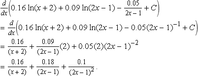
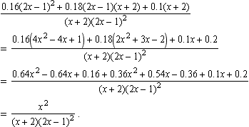
∫x2(x+2)(2x−1)2dx=∫0.16x+2+0.18(2x−1)+0.1(2x−1)2dx=0.16ln(x+2)+0.182ln(2x−1)−0.12(2x−1)−1+C=0.16?ln(x+2)+0.09ln(2x−1)−0.05(2x−1)+C.

Check:
ddx(0.16ln(x+2)+0.09ln(2x−1)−0.052x−1+C)=ddx(0.16ln(x+2)+0.09ln(2x−1)−0.05(2x−1)−1+C)=0.16(x+2)+0.09(2x−1)(2)+0.05(2)(2x−1)−2=0.16(x+2)+0.18(2x−1)+0.1(2x−1)2.
Writing this over a common denominator gives
0.16(2x−1)2+0.18(2x−1)(x+2)+0.1(x+2)(x+2)(2x−1)2=0.16(4x2−4x+1)+0.18(2x2+3x−2)+0.1x+0.2(x+2)(2x−1)2=0.64x2−0.64x+0.16+0.36x2+0.54x−0.36+0.1x+0.2(x+2)(2x−1)2=x2(x+2)(2x−1)2.
8.6 Summary
1. Many physical situations involve exponential growth or decay where the rate of change of y is proportional to its current value.
2. All exponential functions, y = at, are such that d y/dt = ky, that is, the derivative of an exponential function is also an exponential function scaled by a factor k.
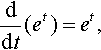
3. The exponential function y = ethas the property that dy/dt = y, that is, its derivative is equal to the original function:
ddt(et)=et,
where e ≈ 2.71828. The inverse function to et is loge(t), which is abbreviated to In(t). This is called the natural or Napierian logarithm.
4. The general solution to d y/dt = ky is y = y0ekt, where y0 is the value of y at t = 0
5.
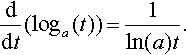
ddt(t)=ln(a)at?and

ddt(loga(t))=1ln(a)t.
6. The hyperbolic cosine (cosh) and hyperbolic sine (sinh) are the even and odd parts of the exponential function:
ex=cosh(x)+sinh(x)
![]()
cosh(x)=ex+e−x2

sinh(x)=ex-e−x2

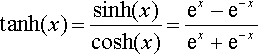
These functions get the name hyperbolic because of their relationship to a hyperbola. The hyperbolic tangent is defined by
tanh(x)=sinh(x)cosh(x)=ex-e−xex+e−x
There are various hyperbolic identities, which are similar to the trigonometric identities (Table 8.2).
7. The inverse hyperbolic functions cosh−1(x)(x ≥ 1), sinh−1(x), tanh −1 (x) (−1 < x < 1) have the following logarithmic identities:
sinh−1(x)=ln(x+√x2+1)?for?all?x∈ℝ
![]()
cosh−1(x)=ln(x+√x2−1)??x≥1
![]()
tan−1(x)=12ln(1+x1−x)?????−1?<x<1

cosh−1 (x) is the inverse of cosh(x) if the domain of cosh(x) is limited to the positive values of x and zero.
8. Adding the derivatives and integrals of the exponential, In, hyperbolic and inverse hyperbolic functions to the tables of standard derivatives and integrals gives Tables 8.3 and 8.4.
9. Partial fractions can be used to integrate fractional functions such as
x+1(x−1)(x+2).

8.7 Exercises
8.1 Using ddt(et)=et show that the function 2e3t is a solution to the differential equation
dydt3y
![]()
8.2 Assuming p = poekt find Po and k such that
dpdt=p1200

and p = 1 when t = 0.
8.3 Assuming N = N0ekt find N0 and k such that
dNdt=−4.3×10⁻⁴N???and????N=5×10⁶??at?t=0.
8.4. Assuming ϕ = Aekt + 300 find A and k such that
dϕdt=−0.1×(ϕ−300)???and????ϕ=400??when?t=0.

8.5. Using the definitions of
cosh(x)=ex+e−x2
and
sinh(x)=ex-e−x2
show that
(b) sinh(x – y) = sinh (x) cosh(y) – cosh(x) sinh(y)
8.6 Using y = tanh−l (x) ⇔ tanh(y) = x, where −1 < x < 1, and
tanh(y)=ey−e−yey+e−y

show that
tanh−1(x)=12ln(1+x1−x)

where −1 < x < 1.
8.7 Calculate the following and where possible use the appropriate inverse functions to check your result:
(b) tanh(3)
(c) sinh−l(0.6)
(d) tanh−l (1.5)
(e) cosh−l (−1.5)
8.8. Differentiate the following:
(b) x = e−t cosh(2t)
(c)
x2−1sinh(x)

(d) In(x3 – 3x) sinh (x)
(e) log2 (2x)
(f) a4t
(g) 2tt2
(h) 1/(et−1)2
8.9 Find the following integrals:
(b) ∫32dt4t−1![]()
(c) ∫x?sin(2x2)dx![]()
(d) ∫x?ln(x)dx![]()
(e) ∫10exx2?dx![]()
(f) ∫sinh(t)cosh(t)dt
(g) ∫2(x−1)x2−2x−4dx![]()
(h) ∫t+1(t−3)(t−1)dt![]()
(i) ∫42−tt2(t−1)dt![]()
8.10. The charge on a discharging capacitor in an RC circuit decays according to the expression Q = 0.001e−10t. Find an expression for the current using I = dQ/dt and find after how long the current is half of its initial value.
8.11 A charging capacitor in an RC circuit with a d.c. voltage of 5 V charges according to the expression q=0.005(1-e-0.5t)![]() . Given that the current i = dq/dt, calculate the current: (a) when t = 0; (b) after 10 s; and (c) after 20 s.
. Given that the current i = dq/dt, calculate the current: (a) when t = 0; (b) after 10 s; and (c) after 20 s.