
Functions and their graphs
2.1 Introduction
The ability to produce a picture of a problem is an important step towards solving it. From the graph of a function, y = f (x), we are able to predict such things as the number of solutions to the equation f(x) = 0, regions over which it is increasing or decreasing, and the points where it is not defined.
Recognizing the shape of functions is an important and useful skill. Oscilloscopes give a graphical representation of voltage against time, from which we may be able to predict an expression for the voltage. The increasing use of signal processing means that many problems involve analysing how functions of time are effected by passing through some mechanical or electrical system.
In order to draw graphs of a large number of functions, we need only remember a few key graphs and appreciate simple ideas about transformations. A sketch of a graph is one which is not necessarily drawn strictly to scale but shows its important features. We shall start by looking at special properties of the straight line (linear function) and the quadratic. Then we look at the graphs of y = x, y = x2, y = 1/x, y = axand how to transform these graphs to get graphs of functions like y = 4 x − 2, y = (x − 2)2, y = 3/x, and y = a−x.
2.2 The straight line: y = mx + c
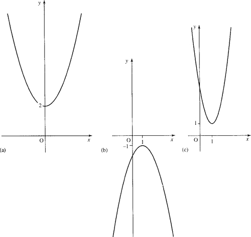
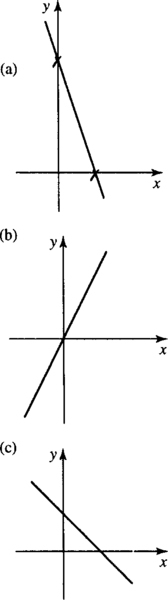
y = mx + c is called a linear function because its graph is a straight line. Notice that there are only two terms in the function; the x term, mx, where m is called the coefficient of x and c which is the constant term. m and c have special significance. m is the gradient, or the slope, of the line and c is the value of y when x = 0, that is, when the graph crosses the y-axis. This graph is shown in Figure 2.1(a) and two particular examples shown in Figure 2.1(b) and (c).

The gradient of a straight line
The gradient gives an idea of how steep the climb is as we travel along the line of the graph. If the gradient is positive then we are travelling uphill as we move from left to right and if the gradient is negative then we are travelling downhill. If the gradient is zero then we are on flat ground. The gradient gives the amount that y increases when x increases by 1 unit. A straight line always has the same slope at whatever point it is measured. To show that in the expression y = mx + c, m is the gradient, we begin with a couple of examples as in Figure 2.1(b) and (c)
In Figure 2.1(b), we have the graph of y = 2x + 3. Take any two values of x which differ by 1 unit, for example, x = 0 and x = 1. When x = 0, y = 2 × 0 + 3 = 3 and when x = 1, y = 2 × 1 + 3 = 5. The increase in y is 5 – 3 = 2, and this is the same as the coefficient of x in the function expression.
In Figure 2.1(c), we see the graph of y = −x + 2. Take any two values of x which differ by 1 unit, for example, x = 1 and x = 2. When x = 1,y = −(1) + 2 = 1 and when x = 2,y = −(2) + 2 = 0. The increase in y is 0–1 = −1 and this is the same as the coefficient of x in the function expression.
In the general case, y = mx + c, take any two values of x which differ by 1 unit, for example, x = x0 and x = x0 + 1. When x = x0, y = mx0+c and when x = x0 + 1, y = m(x + 1) + c = mx + m + c. The increase in y is mx + m + c − (mx + c) = m.
We know that every time x increases by 1 unit y increases by m. However, we do not need to always consider an increase of exactly 1 unit in x. The gradient gives the ratio of the increase in y to the increase in x. Therefore, if we only have a graph and we need to find the gradient then we can use any two points that lie on the line.
To find the gradient of the line take any two points on the line (x1, y1) and (x2, y2).
![]()
Example 2.1
Find the gradient of the lines given in Figure 2.2(a)–(c) and the equation for the line in each case.
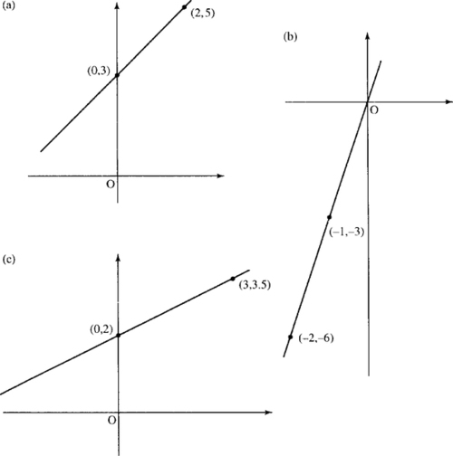
(a) We are given the coordinates of two points that lie on the straight line in Figure 2.2(a) as (0,3) and (2,5),

To find the constant term in the expression y = mx + c, we find the value of y when the line crosses the y-axis. From the graph this is 3, so the equation is y = mx + c where m = 1 and c = 3, giving
![]()
(b) Two points that lie on the line in Figure 2.2(b) are (−1, −3) and (−2, −6). These are found by measuring the x and y values for some points on the line.

To find the constant term in the expression y = mx + c, we find the value of y when the line crosses the y-axis. From the graph this is 0, so the equation is y = mx + c where m = 3 and c = 0 giving y = 3x
(c) Two points that lie on the line in Figure 2.2(c) are (0,2) and (3,3.5).

To find the constant term in the expression y = mx + c, we find the value of y when the line crosses the y-axis. From the graph this is 2, so the equation is y = mx + c where m = 0.5 and c = 2 giving
![]()
Finding the gradient from the equation for the line
To find the gradient from the equation of the line we look for the value of m, the number multiplying x in the equation. The constant term gives the value of y when the graph crosses the y-axis, that is, when x = 0.
Example 2.2
Find the gradient and the value of y when x = 0 for the following lines:
Solution
(a) In the equation y = 2x + 3, the value of m, the gradient, is 2 as this is the coefficient of x. c = 3 which is the value of y when the graph crosses the y-axis, that is, when x = 0.
(b) In the equation 3x − 4 y = 2, we rewrite the equation with y as the subject of the formula in order to find the value of m and c.

We can see, by comparing the expression with y = mx + c, that m, the gradient, is 3/4 and c = −1/2.
(c) Write y as the subject of the formula:

We can see, by comparing the expression with y = mx + c, that m, the gradient, is 1/2 and c = −2.
(d) Write y as the subject of the formula

We can see, by comparing the expression with y = mx + c, that m, the gradient, is − 3 /2 and c = 9/2.
Finding the equation of a line which goes through two points
Supposing we have been given two points, (x1, y1) and (x2, y2), which lie on a line and we want to find the equation of that line. We already found that the gradient of the line is given by:
We know that the equation of a line is of the form y = mx + c, but we would like to express the equation just in terms of the two variables, x and y, and the known points which the line passes through, (x1, y1) and (x2, y2). To do this we use the fact that a line is of constant gradient. That means that for any point (x, y), the gradient between (x, y) and the point (x1, y1) must be the same as the gradient between (x1, y1) and the point (x2, y2). This gives:
providing that y2 ≠ y1, we can rearrange this equation as:

Note that if y2 = y1 and we have chosen two different points on the line, that is, x2 ≠ x1 then y is a constant and the equation of the line will be y = y1.
Example 2.3
(a) Find the equation of a line through the points (2,4) and (0,6).
(b) Find the equation of a line through the points (1, −6) and (5, −6).
Solution
(a) To find the equation of a line through the points (2,4) and (0,6) we use

This gives
Check: Check that this is the correct equation by substituting the points (2,4) and (0,6) into the equation y = −x + 6. (2,4) gives 4 = −2 + 6 ⇔4 = 4, which is true; (0,6) gives 6 = −0 + 6, which is true.
This shows that y = −x + 6 is the equation of a straight line which goes through the points (2,4) and (0,6).
(b) To find the equation of a line through the points (1, −6) and (5, −6) we try to use (y − y1) / (y2 − y1) = (x − x1) / (x2 − x1) with (x1, y1) = (1, −6) and (x2, y2) = (5, −6) but find that, because y2 = y1, the substitution would result in a division by 0, which is undefined. We note that y has constant value and therefore the equation of the line is:
![]()
Sketching a straight line graph
The quickest way to sketch a straight line graph is to find the points where it crosses the axes. However, any two points on the graph can be used and sometimes it is more convenient to find other points.
Example 2.4
(a) Sketch the graph of y = 4x − 2.
To find where the graph crosses the y-axis, substitute x = 0 into the equation of the line:
![]()
This means that the graph passes through the point (0,−2). To find where the graph crosses the x-axis, substitute y = 0, that is,
Therefore, the graph passes through (0.5, 0).
Mark the points (0,2) and (0.5,0), on the x- and y-axes and join the two points. This is done in Figure 2.3(a).

(b) Sketch the graph of y = −4x When x = 0 we get y = 0, that is the graph goes through the point (0,0). In this case, as the graph passes through the origin, we need to choose a different value for x for the second point. Taking x = 2 gives y = −8, so another point is (2, −8). These points on marked on the graph and joined to give the graph as in Figure 2.3(b).
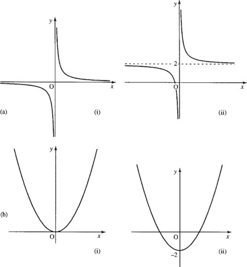
2.3 The quadratic function: y = ax2+bx+c
y = ax2+ bx + c is a general way of writing a function in which the highest power of x is a squared term. This is called the quadratic function and its graph is called a parabola as shown in Figure 2.4.

All the graphs, in this figure, cross the y-axis at (0, c). To find where they cross the x-axis can be more difficult. These values, where f(x) = 0, are called the roots of the equation. There is a quick way to discover whether the function crosses the x-axis, only touches the x-axis, or does not cross or touch it. In the latter case there are no solutions to the equation f(x) = 0. The three possibilities are given in Figure 2.4.
Crossing the x-axis
The function y = ax2+ bx + c crosses the x-axis when y = 0, that is, when ax2+bx+c = 0. The solutions to ax2+bx+c = 0 are examined in the Background Mathematics Notes available on the companion website for this book and are given by the formula
From the graph, we can see there are three possibilities:
1. In Figure 2.4(a) where there are two solutions, that is, the graph crosses the x-axis for two values of x. For this to happen, the square root part of the formula above must be greater than zero:
![]()
Examples are given in Figure 2.5.

2. Only one unique solution, as in Figure 2.4(b). The graph touches the x-axis in one place only. For this to happen, the square root part of the formula must be exactly 0. Examples of this are given in Figure 2.6.

3. No real solutions, that is, the graph does not cross the x-axis. Examples of these are given in Figure 2.7.
2.4 The function y = 1/x
The function y = 1/x has the graph as in Figure 2.8. This is called a hyperbola. Notice that the domain of f(x) = 1/x does not include x = 0. The graph does not cross the x-axis so there are no solutions to 1/x = 0.

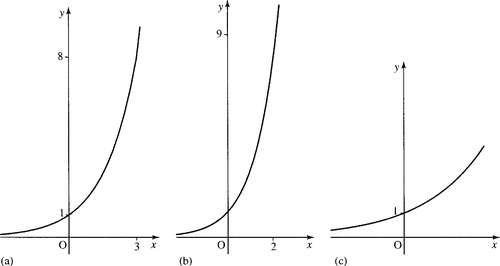
2.5 The functions y = ax
Graphs of exponential functions, y = ax, are shown in Figure 2.9. The functions have the same shape for all a > 1. Notice that the function is always positive and the graph does not cross the x-axis so there are no solutions to the equation ax= 0.
2.6 Graph sketching using simple transformations
One way of sketching graphs is to remember the graphs of simple functions and to translate, reflect or scale those graphs to get graphs of other functions. We begin with the graphs below as given in Figure 2.10.

The translation x  x + a
x + a
If we have the graph of y = f(x), then the graph of y = f(x + a) is found by translating the graph of y = f(x) a units to the left. Examples are given in Figure 2.11.

The translation f(x) (x) + A
Adding A on to the function value leads to a translation of A units upwards. Examples are given in Figure 2.12.
Reflection about the y-axis, x −x
Replacing x by −x in the function has the effect of reflecting the graph in the y-axis – that is, as though a mirror has been placed along the axis and only the reflection can be seen. Examples are given in Figure 2.13.

Reflection about the x axis, f(x) −f(x)
To find the graph of y = − f(x), reflect the graph of y = f(x) about the x-axis. Examples are given in Figure 2.14.

Scaling along the x-axis, x ax
Multiplying the values of x by a number, a, has the effect of: squashing the graph horizontally if a > 1 or stretching the graph horizontally if o < a < 1. Examples are given in Figure 2.15.

Scaling along the y-axis, f(x) Af(x)
Multiplying the function value by a number A has the effect of stretching the graph vertically if A > 1, or squashing the graph vertically if 0 < A < 1. Examples are given in Figure 2.16.

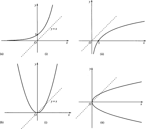
Reflecting in the line y = x
If the graph of a function y = f(x) is reflected in the line y = x, then it will give the graph of the inverse relation. Examples are given in Figure 2.17.
 . The second graph is found by reflecting the first graph in the line y = x. Notice that
  is not a function as there is more that one possible value of y for each value of x > 0.
In Chapter 1, we defined the inverse function as taking any image back to its original value. Check this with the graph of y = 2xin Figure 2.17(a): x = 1 gives y = 2. In the inverse function, y = log2 (x), substitute 2, which gives the result of 1, which is back to the original value.
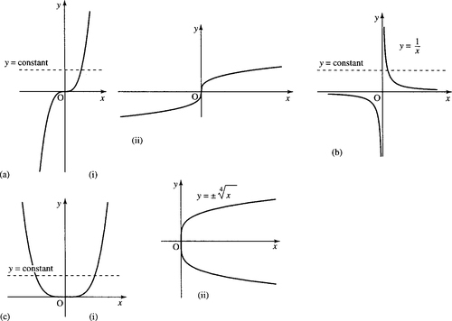
However, the inverse of y = x2, y ± ![]() , shown in Figure 2.17(b), is not a function as there is more than one y value for a single value of x. To understand this problem more fully, perform the following experiment. On a calculator enter −2 and square it (x2) giving 4. Now take the square root. This gives the answer 2, which is not the number we first started with, and hence we can see that the square root is not a true inverse of squaring. However, we get away with calling it the inverse because it works if only positive values of x are considered. To test if the inverse of any function exists, draw a line along any value of y = constant. If, wherever the line is drawn, there is ever more than one x value which gives the same value of y then the function has no inverse function. In this situation, the function is called a ‘many-to-one’ function. Only ‘one-to-one’ functions have inverses. Figure 2.18 has examples of functions with an explanation of whether they are ‘one-to-one’ or ‘many-to-one’.
, shown in Figure 2.17(b), is not a function as there is more than one y value for a single value of x. To understand this problem more fully, perform the following experiment. On a calculator enter −2 and square it (x2) giving 4. Now take the square root. This gives the answer 2, which is not the number we first started with, and hence we can see that the square root is not a true inverse of squaring. However, we get away with calling it the inverse because it works if only positive values of x are considered. To test if the inverse of any function exists, draw a line along any value of y = constant. If, wherever the line is drawn, there is ever more than one x value which gives the same value of y then the function has no inverse function. In this situation, the function is called a ‘many-to-one’ function. Only ‘one-to-one’ functions have inverses. Figure 2.18 has examples of functions with an explanation of whether they are ‘one-to-one’ or ‘many-to-one’.
 .
.2.7 The modulus function, y = |x| or y = abs(x)
The modulus function y = |x|, often written as y = abs(x) (short for the absolute value of x) is defined by

The output from the modulus function is always a positive number or zero.
Example 2.5
Find |−3|. Here x = −3, which is negative, therefore
![]()
An alternative way of thinking of it is to remember that the modulus is always positive, or zero, so simply replacing any negative sign by a positive one will give a number's modulus or absolute value.
![]()
The graph of the modulus function can be found from the graph of y = x by reflecting the negative x part of the graph to make the function values positive. This is shown in Figure 2.19.

2.8 Symmetry of functions and their graphs
Functions can be classified as even, odd, or neither of these.
Even functions
Even functions are those that can be reflected in the y-axis and then result in the same graph. Examples of even functions are (see Figure 2.20):
![]()

As previously discussed, reflecting in the y-axis results from replacing x by −x in the function expression and hence the condition for a function to be even is that substituting −x for x does not change the function expression, that is, f(x) = f (− x).
Example 2.6
Show that 3x2 − x4 is an even function. Substitute −x for x in the expression f(x) = 3x2 − x4 and we get
![]()
So, we have found that f (− x) = f(x) and therefore the function is even.
Odd functions
Odd functions are those that when reflected in the y-axis result in an upside down version of the same graph. Examples of odd functions are (see Figure 2.21):
![]()

Reflecting in the y-axis results from replacing x by −x in the function expression and the upside down version of the function f(x) is found by multiplying the function by −1. Hence, the condition for a function to be odd is that substituting −x for x gives − f(x), that is,
![]()
Example 2.7
Show that 4x–(1/x) is an odd function. Substitute x for –x in the expression f(x) = 4x – (1/x) and we get
We have found that f(−x) = −f(x), so the function is odd.
2.9 Solving inequalities
For linear and quadratic functions, y = f(x), we have discussed how to find the values where the graph of the functions crosses the x-axis, that is how to solve the equation f(x) = 0. It is often of interest to find ranges of values of x where f(x) is negative or where f(x) is positive. This means solving inequalities like f(x) < 0 or f(x) > 0, respectively.
Like equations, inequalities can be solved by looking for equivalent inequalities. One way of finding these is by doing the same thing to both sides of the expression. There is an important exception for inequalities that if both sides are multiplied or divided by a negative number then the direction of the inequality must be reversed.
To demonstrate these equivalences begin with a true proposition
![]()
Add 2 on to both sides and it is still true
![]()
Subtract 10 from both sides and we get
![]()
which is also true.
Multiply both sides by −1 and if we do not reverse the inequality we get
![]()
which is false. However, if we use the correct rule that when multiplying by a negative number we must reverse the inequality sign then we get:
![]()
which is true. This process is pictured in Figure 2.22.
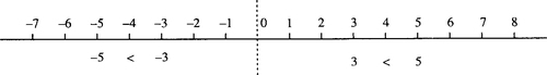
Note that inequalities can be read from right to left as well as from left to right: 3 < 5 can be read as ‘3 is less than 5’ or as ‘5 is greater than 3’ and so it can also be written the other way round as 5 > 3.
Using a number line to represent inequalities
An inequality can be expressed using a number line as in Figure 2.23. In Figure 2.23(a), the open circle indicates that 3 is not included in the set of values, t < 3. In Figure 2.23(b), the closed circle indicates that −2 is included in the set of values, x ≥ −2. In Figure 2.23(c), the closed circle indicates that the value 4.5 is included in the set y ≤ 4.5.

Example 2.8
Find a range of values for t, x, and y such that the following inequalities hold
(b) x + 5 ≥ 4x − 10
(c) 16 − y > −5y
Solution
(a) 2t + 3 < t − 6 ⇔2t − t + 3 < −6 (subtract t from both sides)
⇔ t < −6–3 (subtract 3 from both sides)
⇔ t < −9.
This solution can be represented on a number line as in Figure 2.24.

(b) x+5 ≥ 4x−10
⇔+5≥ 3x − 10 (subtract x from both sides)
⇔15≥ 3x (add 10 to both sides)
⇔5≥ x (divide both sides by 3)
⇔x ≤5.
This solution in represented in Figure 2.25.

(c) 16 − y > −5y
⇔ 16 > −4y (add y to both sides)
⇔ −4 < y (divide by − 4 and reverse the sign)
⇔ y > −4.
This solution is represented in Figure 2.26.

Representing compound inequalities on a number line
We sometimes need a picture of the range of values given if two inequalities hold simultaneously, for instance x ≥ 3 and x < 5. This is analysed in Figure 2.27(a) and we can see that for both inequalities to hold simultaneously x must lie in the overlapping region where 3 ≤ x < 5. 3 ≤ x < 5 is a way of expressing that x lies between 3 and 5 or is equal to 3. In the example in Figure 2.27(b), x > 6 and x > 2, and for them both to hold then x > 6.

Another possible way of combining inequalities is to say that one or another inequality holds. Examples of this are given in Figure 2.27(c) where x < 5 or x ≥ 7 and this gives the set of values less than 5 or greater than or equal to 7. Figure 2.27(d) gives the example where x < 2 or x ≥ 0 and in this case it results in all numbers lying on the number line, that is, x ∈ ![]() .
.
Example 2.9
Find solutions to the following combinations of inequal- ities and represent them on a number line.
(b) 1−u<3u+2 or μ+2≥6,
(c) t + 5 > 12 and −t > 24.
Solution
(a) x + 3 > 4 and x−1 < 5 We solve both inequalities separately and then combine their solution sets

So the combined inequality giving the solution is x > 1 and x < 6. which from Figure 2.28(a) we can see is the same as 1 < x < 6.
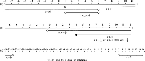
(b) 1 − u < 3u + 2 or u + 2 ≥6
We solve both inequalities separately and then combine their solution sets,

Combining the two solutions gives u > −1/4 or u ≥ 4 and this is represented on the number line in Figure 2.28(b) where we can see that it is the same as u > −1/4.
(c)
Combining the two solutions sets gives t > 7 and t < − 24 and we can see from Figure 2.28(c) that this is impossible and hence there are no solutions.
Solving more difficult inequalities
To solve more difficult inequalities, our ideas about equivalence are not enough on their own, we also use our knowledge about continuous functions. In the previous chapter, we defined a continuous function as one that could be drawn without taking the pen off the paper. If we wish to solve the inequality f(x) > 0 and we know that f(x) is continuous then we can picture the problem graphically as in Figure 2.29. From the graph we can see that to solve the inequality we need only find the values where f(x) = 0 (the roots of f(x) = 0) and determine whether f(x) is positive or negative between the values of x where f(x) = 0. To do this, we can use any value of x between the roots. We are using the fact that as f(x) is continuous then it can only change from positive to negative by going through zero.

Example 2.10
Find the values of t such that t2 − 3t < − 2. Write the inequality with 0 on one side of the inequality sign
![]()
Find the solutions to f(t) = t2 − 3t + 2 = 0 and mark them on a number line as in Figure 2.30.
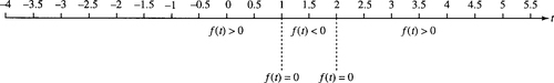
Using the formula

where a = 1, b = −3, and c = 2 gives

Substitute values for t which lie on either side of the roots of f(t) in order to find the sign of the function between the roots. Here we choose 0, 1.5, and 3.
When t = 0
![]()
which is positive, giving f(t) > 0. When t = 1.5
![]()
which is negative giving f(t) < 0. When t = 3
![]()
which is positive, giving f(t) > 0.
By marking the regions on the number line, given in Figure 2.30, with f(t) > 0, f(t) < 0, or f(t) = 0 as appropriate we can now find the solution to our inequality f(t) < 0 which is given by the region where 1 < t < 2.
Example 2.11
Find the values of x such that (x2 − 4)(x + 1) > 0.
Solution The inequality already has 0 on one side of the inequality sign so we begin by finding the roots to f(x) = 0, that is,
![]()
Factorization gives
![]()
⇔ x = 2, x = −2, or x = −1. So the roots are −2, −1, and 2. These roots are pictured on the number line in Figure 2.31.
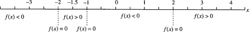
Substitute values for x which lie on either side of the roots of f(x) in order to find the sign of the function between the roots. Here we choose −3, −1.5, 0, and 2.5.
When x = −3

When x = 1.5

When x = 0

When x = 2.5
These regions are marked on the number line as in Figure 2.31 and the solution is given by those regions where f(x) > 0 Looking for the regions where f(x) > 0 gives the solution as − 2 < x < −1 or x > 2.
2.10 Using graphs to find an expression for the function from experimental data
Linear relationships
Linear relationships are the easiest ones to determine from experimental data. The points are plotted on a graph and if they appear to follow a straight line then a line can be drawn by hand and the equation can be found using the method given in Section 2.2.
Example 2.12
A spring is stretched by hanging various weights on it and in each case the length of the spring is measured.
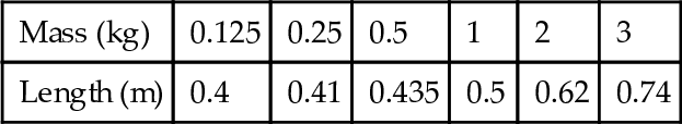
Approximate the length of the spring when no weight is hung from it and find the expression for the length in terms of the mass.
Solution First, draw a graph of the given experimental data. This is done in Figure 2.32.

A line is fitted by eye to the data. The data does not lie exactly on a line due to experimental error and due to slight distortion of the spring with heavier weights. From the line we have drawn we can find the gradient by choosing any two points on the line and calculating

Taking the two points as (0,0.28) and (2,0.58), we get the gradient as
![]()
The point where it crosses the y-axis, that is, where the mass hung on the spring is 0 can be found by extending the line until it crosses the y-axis. This gives 0.38 m.
Finally, the expression for the length in terms of the mass of the attached weight is given by y = mx + c, where y is the length and x is the mass,
m is the gradient and c is the value of y when x = 0, that is, where there is no weight on the string. This gives
length = 0.1 × mass + 0.38
The initial length of the spring is 0.38 m.
Exponential relationships
Many practical relationships behave exponentially particularly those involving growth or decay. Here it is slightly less easy to find the relationship from the experimental data, however, it is simplified by using a log–linear plot. Instead of plotting the values of the dependent variable, y, we plot the values of log10(y). If the relationship between y and time, t, is exponential as we suspected then the log10(y) against t plot will be a straight line.
The reason this works can be explained as follows. Supposing y = y0 10kt where y0 is the value of y when t = 0 and k is some constant; then, taking the log base 10 of both sides, we get
As the logarithm base 10 and raising to the power of 10 are inverse operations, we get
![]()
As y0 is a constant, the initial value of y, and k is a constant then we can see that this expression shows that we shall get a straight line if log10 (y) is plotted against t. The constant k is given by the gradient of the line and log10(y0) is the value of log10(y) where it crosses the vertical axis. Setting Y = log10(y), c = log10(y0)
![]()
which is the equation of the straight line.
Example 2.13
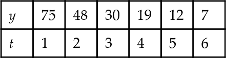
A room was tested for its acoustical absorption properties by playing a single note on a trombone. Once the sound had reached its maximum intensity, the player stopped and the sound intensity was measured for the next 0.2 s at regular intervals of 0.02 s. The initial maximum intensity at time 0 is 1.0. The readings were as follows:

Draw a graph of intensity against time and log (intensity) against time and use the latter plot to approximate the relationship between the intensity and time.
Solution The graphs are plotted in Figure 2.33 where, for the second graph (b), we take the log10 (intensity) and use the table below:

| Time | 0 0.02 | 0.04 | 0.06 | 0.08 | 0.1 | 0.12 | 0.14 | 0.16 | 0.18 | 0.2 |
| log10 (intensity) | 0–0.22 | –0.46 | –0.66 | –0.89 | –1.1 | –1.3 | –1.5 | –1.7 | –2 | –2.3 |

We can see that the second graph is approximately a straight line and therefore we can assume that the relationship between the intensity and time is exponential and could be expressed as I = I010kt. The log10 of this gives
![]()
From the graph in Figure 2.33(b), we can measure the gradient, k. To do this we calculate

giving
![]()
The point at which it crosses the vertical axis gives
![]()
Therefore, the expression I = I0 10kt becomes
![]()
Power relationships
Another common type of relationship between quantities is when there is a power of the independent variable involved. In this case, if y = axn where n could be positive or negative then the value of a and n can be found by drawing a log–log plot.
This is because taking log10 of both sides of y = axn gives
![]()
Replacing Y = log10(y) and X = log10(x) we get:
![]()
showing that the log–log plot will give a straight line, where the slope of the line will give the power of x and the position where the line crosses the vertical axis will give the log10(a). Having found a and n, they can be substituted back into the expression
![]()
Example 2.14
The power received from a beacon antenna is though to depend on the inverse square of the distance from the antenna and the receiver. Various measurements, given below, were taken of the power received against distance r from the antenna. Could these be used to justify the inverse square law? If so, what is the constant, A, in the expression:
![]()

Solution To test whether the relationship is indeed a power relationship we draw a log−log plot. The table of values is found below:
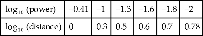
Graphs of power against distance and log10(power) against log10(distance) are given in Figure 2.34(a) and (b).

As the second graph is a straight line, we can assume that the relationship is of the form P = Arn where P is the power and r is the distance, In which case, the log–log graph is
![]()
We can measure the slope by calculating
and, using the two points that have been found to lie on the line, this gives
As this is very near to − 2, the inverse square law would appear to be justified.
The value of log10(A) is given from where the graph crosses the vertical axis and this gives
![]()
So the relationship between power received and distance is approximately
![]()
2.11 Summary
1. The linear function y = mx + c has gradient (slope) m and crosses the y-axis at y = c.
2. The gradient, m, of a straight line y = mx + c is given by:
and this is the same along the length of the line.
3. The equation of a line which goes through two points, (x1, y1) and (x2, y2) is:

4. The graph of the quadratic function y = ax2 + bx + c is called a parabola. The graph crosses the y-axis (when x = 0) at y = c.
5. There are three possibilities for the roots of the quadratic equation a x2+ bx + c = 0
Case I: two real roots when b2 − 4ac > 0,
Case II: only one unique root when b2 − 4ac = 0,
Case III: no real roots when b2 − 4ac < 0.
6. By considering the graphs of known functions y = f(x), for instance, those given in Figure 2.10, and the following transfor-mations, many other graphs can be drawn.
(a) Replacing x by x + a in the function y = f(x) results in shifting the graph a units to the left.
(b) Replacing f(x) by f(x) + A results in shifting the graph A units upwards.
(c) Replacing x by −x reflects the graph in the y-axis.
(d) Replacing f(x) by − f(x) reflects the graph in the x-axis (turning it upside down).
(e) Replacing x by ax squashes the graph horizontally if a > 1 or stretches it horizontally if 0 < a < 1.
(f) Replacing f(x) by Af(x) stretches the graph vertically if A > 1 or squashes it vertically if 0 < A < 1.
(g) Reflecting the graph of y = f(x) in the line y = x results in the graph of the inverse relation.
7. A function may be even, or odd, or neither of these.
(a) An even function is one whose graph remains the same if reflected inthe y-axis, that is, when x ![]() −x. This can also be expressed by the condition
−x. This can also be expressed by the condition
![]()
Examples of even functions are y = x2, y = |x|, and y = x4.
(b) An odd function is one which when reflected in the y-axis, that is, when x ![]() −x, gives an upside down version of the original graph (i.e. − f(x)). This can also be expressed as the condition:
−x, gives an upside down version of the original graph (i.e. − f(x)). This can also be expressed as the condition:
![]()
Examples of odd functions are y = x and y = x3.
8. Not all functions have true inverses. Only one-to-one functions have inverse functions. A function is one-to-one if any line y = constant drawn on the graph y = f(x) crosses the function only once. This means there is exactly one value of x that gives each value of y.
9. Simple inequalities can be solved by finding equivalent inequalities. Inequalities remain equivalent if both sides of the inequality have the same expression added or subtracted. They may also be multiplied or divided by a positive number but if they are multiplied or divided by a negative number then the direction of the inequality sign must be reversed.
10. To solve the inequalities f(x) > 0, f(x) < 0, f(x) ≤ 0, or f(x) ≥ 0, where f(x) is a continuous function, solve f(x) = 0 and choose any value for x around the roots to find the sign of f(x) for each region of values for x.
11. Graphs can be used to find relationships in experimental data. First, plot the data then:
(a) If the data lies on an approximate straight line then draw a straight line through the data and find the equation of the line.
(b) If it looks exponential, then take the log of the values of the dependent variable and draw a log–linear graph. If this looks approximately like a straight line then assume there is an exponential relationship y = y0 10kt, where k is given by the gradient of the line and log10(y0) is the value where the graph crosses the vertical axis.
(c) If the relationship looks something like a power relationship, y = Axn, then take the log of both sets of data and draw a log–log graph. If this is approximately like a straight line, then assume there is a power relationship and n is given by the gradient of the line and log10A is the value where the graph crosses the vertical axis.
2.12 Exercises
2.1. Sketch the graphs of the following:
In each case state the gradient of the line.
2.2. A straight line passes through the pair of points given. Find the gradient of the line in each case.
2.3. A straight line graph has gradient −5 and passes through (1,6). Find the equation of the line.
2.4. In Figure 2.35 are various graphs drawn to the scale 1 unit = 1 cm. By finding the gradients of the lines and where they cross the y-axis, find the equation of the line.
2.5. A straight line passes through the pair of points given. Find the equation of the line in each case.
2.6. Find the values of x such that f (x) = 0 for the following functions
(b) f(x) = (2x − 1)(x + 1),
(c) f(x) = (x − 3)2,
(d) f(x) = (x − 4)(x + 4),
(e) f(x) = x2 + x − 6,
(f) f(x) = x2 + 7 x + 12,
(g) f(x) = 12 x2 − 12 x − 144.
Using the fact that the peak or trough in the parabola, y = f(x), occurs at a value of x half-way between the values where f(x) = 0 then sketch graphs of the above quadratic functions.
2.7. By considering transformations of simple functions sketch graphs of the following:

2.8. Consider reflections of the graphs given in Figure 2.36 to determine whether they are even, odd, or neither of these.

2.9. By substituting x ![]() −x in the following functions determine whether they are odd, even, or neither of these:
−x in the following functions determine whether they are odd, even, or neither of these:
2.10. Draw graphs of the following functions and draw the graph of the inverse relation in each case. Is the inverse a function?

2.11. Find the range of values for which the following inequalities hold and represent them on a number line.
(b) 10x − 3x > −2,
(c) 3–4 y ≥ 11 + y,
(d) t + 15 < 6 − 2t.
2.12. Find the range of values for which the following hold and represent them on a number line:
(b) 4t + 2 ≥ 10 and 3 − 2t < 1,
(c) 3 u + 10 > 16 or 3 − 2u > 13.
2.13. Solve the following inequalities and represent the solutions on a number line:
(b) (2x − 3) (x + 1) (x − 5) > 0,
(c) t2 + 4t ≤ 21,
(d) 4w2+ 4w − 35 ≥ 0.
2.14. For the following sets of data, y is thought to depend exponentially on t. Draw log–linear graphs in each case and find constants A and k such that y = A10kt.
(b)

2.15. An experiment measuring the change in volume of a gas as the pressure is decreased gave the following measurements:
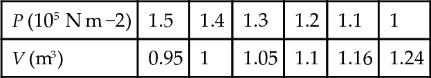
If the gas is assumed to be ideal and the expansion is adiabatic then the relationship between pressure and volume should be:
![]()
where y and C are constants and p is the pressure and V is the volume. Find reasonable values of y and C to fit the data and from this expression find the predicted volume at atmospheric pressure, p = 1.013 × 10⁵ N m−2.