
Maxima and minima and sketching functions
11.1 Introduction
Differentiation can be used to examine the behaviour of a function and find regions where it is increasing or decreasing, and where it has maximum and minimum values. For instance, we may be interested in finding the maximum height, maximum power, or generating the maximum profit, or in finding ways to use the minimum amount of energy or minimum use of materials. Maximum and minimum points can also help in the process of sketching a function.
11.2 Stationary points, local maxima and minima
Example 11.1
Throw a stone in the air and initially it will have a positive velocity as the height, s, increases; that is, ds / dt > 0. At some point it will start to fall back to the ground, the distance from the ground is then decreasing, and the velocity is negative, ds / dt < 0. In order to go from a positive velocity to a negative velocity there must be a turning point, where the stone is at its maximum height and the velocity is zero. If the stone has initial velocity 20 ms−1, how can we find the maximum height that it reaches?
In order to express the velocity of the stone we can make the assumption that air resistance is negligible and use the relationship between distance and time for motion under constant acceleration, giving
![]()
where s is the distance travelled, u the initial velocity, t is time, and a the acceleration. In this case, u = 20 ms−1 and a = –g (acceleration due to gravity ≈ 10 ms−2), so s = 20t – 5t2.
At the maximum height, the rate of change of distance with time must be 0, that is, the velocity is 0. Therefore, we differentiate to find the velocity:
Putting υ = 0 gives
![]()
We have shown that the maximum height is reached after 2 s. But what is that height? Substituting t = 2 into the equation for s gives
![]()
giving the maximum value of s as 20 m.
This example illustrates the important step in finding maximum and minimum values of a function, y = f (x). That is, we differentiate and solve
![]()
This may give various values of x. The points where dy / dx = 0 are called the stationary points but having found these we still need a way of deciding whether they could be maximum or minimum values. In the example, we knew that a stone thrown into the air must reach a maximum height and then return to the ground, and so by solving ds / dt = 0 we would find the time at the maximum. Other problems may not be so clear cut and thus we need a method of distinguishing between different types of stationary points.
A stationary point is classified as either a local maximum, a local minimum, or a point of inflexion. The plural of maximum is maxima and the plural of minimum is minima. The word ‘local’ is used in the description, because local maxima or local minima do not necessarily give the overall maximum or minimum values of the function. For instance, in Figure 11.1 there is a local maximum at B, but the value of y at x = x1 is actually bigger; hence, the overall maximum value of the function in the range is given by y at xl.
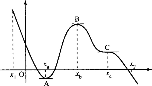
To see how to classify stationary points, examine Figure 11.1, where points A, B, and C are all stationary points.
In order to analyse the slope of the function, imagine the function as representing the cross-section of a mountain range and we are crossing it from left to right.
At points A, B, and C in Figure 11.1, the gradient of the tangent to the curve is zero, that is, dy / dx = 0.
At A there is a local minimum, where the graph changes from going downhill to going uphill.
At B there is a local maximum, where the graph changes from going uphill to going downhill.
At C there is a point of inflexion, where the graph goes flat briefly before resuming its descent.
Local maxima and minima are also called turning points because the function is changing from increasing to decreasing or vice versa.
By looking at where the graph is going uphill, that is, dy/dx > 0, at where it is going downhill, that is, dy/dx < 0, and especially remembering to mark the points where dy/dx = 0, the stationary points, we can draw a very rough sketch of the derivative of any function just by looking at its graph. This we do for our example graph in Figure 11.2. By examining the graph of dy/dx we can see that at a local minimum point dy/dx = 0 and dy/dx is negative just before the minimum and positive afterwards. For a local maximum point dy/dx = 0 and dy/dx is positive just before the maximum and negative afterwards.

If at the point where dy/dx = 0 and the derivative has the same sign on either side of the stationary point then it must be a point of inflexion. (At point C, dy/dx is negative just before and just after x = c.)
Analysing the sign of dy/dx on either side of a stationary point is one way of classifying whether it is a maximum, minimum, or point of inflexion. Another, sometimes quicker way, is to use the derivative of the derivative, the second derivative, d2y/dx2, also referred to as f″ (x).
To understand how to use the second derivative, examine Figure 11.2(b). We can see that at xa, f″ (x) is heading uphill; hence, its slope, f″ (x), is positive. At xb f’ (x) is heading downhill; hence, its slope, f″ (x), is negative. At xc, f’ (x) has zero slope and therefore f″ (x) is 0.
We can now summarize the steps involved in finding and classifying the stationary points of a function y = f (x) and in finding the overall maximum or minimum value of a function.
Step 1 Find the values of x at the stationary points. First, find dy/dx and then solve for x such that dy/dx = 0.
Step 2 To classify the stationary points there is a choice of method, although Method 2 does not always give a conclusive result.
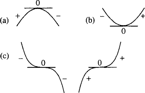
Method 1 For each of the values of x found in Step 1, find out whether the derivative is positive or negative just before the stationary point and just after the stationary point. The classifications are summarized below.
| dy/dx before | → | 0 | → | dy/dx after | Type of stationary point |
| + | → | 0 | → | − | Maximum point |
| − | → | 0 | → | + | Minimum point |
| + | → | 0 | → | + | Point of inflexion |
| − | → | 0 | → | − | Point of inflexion |

These results are summarized in Figure 11.3.
Method 2 Find the second derivative, d2y /dx2 and substitute in turn each of the values of x found in Step 1 (the values of x at the stationary points).
If d2y/dx2 is negative, this indicates that there is a maximum point.
If d2y/dx2 is positive, this indicates that there is a minimum point.
However, if d2y/dx2 = 0, then the test is inconclusive and we must revert to Method 1.
Step 3 Find the values of y at the maximum and minimum points to give the co-ordinates of the turning points.
Step 4 The overall maximum or minimum values of the function can be found in the following way, as long the function is continuous over the values of x of interest. Substitute the boundary values of x into the function to find the corresponding values for y. Compare the values of y found in Step 3 to these boundary values to find the overall maximum and minimum.
Example 11.2
Find and classify the stationary points of y = x3–9x2 +24 x + 3 and find the overall maximum and minimum value of the function in the range x = 0 to x = 5.
Solution
Step 1. First, we must solve dy/dx = 0

So we put

(factorizing to find the roots, although we could also use the formula for solving a quadratic equation if no factorization can easily be found)

Therefore, the stationary points occur when x = 2 or x = 4.
Step 2. To classify these we use Method 2 as outlined above and look at the second derivative, that is, we differentiate dy/dx

At x = 2, d2y/dx2= 12 – 18 = −6, which is negative, showing that at x = 2, f″ (x) is negative and we therefore have a local maximum.
At x = 4, d2y /dx2 = 24 – 18 = 6, which is positive, showing that at x = 4, f″ (x) is positive and we therefore have a local minimum.
Step 3. We still need to know the function value, the value of y at these stationary points. To find the value of y we substitute into the original expression. At x = 2, we get
![]()
Therefore, the local maximum occurs at the point (2,23). At x = 4, we get
![]()
Hence, the local minimum occurs at the point (4,19).
Step 4. To find the overall maximum value and minimum value, substitute the boundary values for x. These are given as x = 0 and x = 5.
At x = 0, y = (0)3 – 9(0)2 + 24(0) + 3 = 0 −0 + 0 + 3 = 3 At x = 5, y = (5)3 – 9(5)2 + 24(5) + 3 = 125 – 225 + 120 + 3 = 23 So the boundary points are (0,3) and (5,23).
Comparing the numbers 3 and 23 with the values of the function at the maximum and minimum in Step 3, that is, 23 and 19, we can see that the overall maximum value occurs at x = 5 and x = 2, where y = 23. The overall minimum value occurs at x = 0, where y = 3. These findings are confirmed by the sketch of the function, which we now have sufficient information to make, as in Figure 11.4.

Example 11.3
Find and classify the stationary points of y = – (2 – x)4.
Solution
Step 1

Stationary points occur where dy/dx = 0:
![]()
Step 2. To classify this stationary point, we differentiate again:
At x = 2, we get d2y/dx2= – 12(2 – 2)2 = 0. So the second derivative is zero.
We cannot use the second derivative test to classify the stationary point because a zero value is inconclusive, so we go back to the first derivative and examine its sign at a value of x just less than x = 2 and just greater than x = 2. This can be done with the help of a table. Choose any values of x less than x = 2 and greater than x = 2, and here we choose x = 1 and x = 3. Be careful if the function is discontinuous at any point not to cross the discontinuity
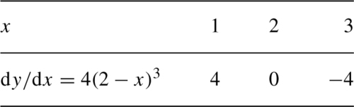
At x = 1, dy/dx = 4(2 – 1)3 = 4 (positive); at x = 3, dy/dx = 4(2 – 3)3 = −4 (negative). Therefore, near the point x = 2 the derivative goes from positive to zero to negative. Therefore, the graph of the function goes from travelling uphill to travelling downhill, showing that we have a maximum value.
Step 3. Finally, we find the value of the function at the maximum point. At x = 2, y = 0, that is, there is a maximum at (2, 0).
Applications of maximum and minimum values of a function
Example 11.4
The power delivered to the load resistance RLfor the circuit shown in Figure 11.5 is defined by


Show that the maximum power delivered to the load occurs for RL = 2000.
Solution For a maximum value dP/dRL= 0

Using the quotient rule to find the derivative we get
As RLis positive 2000 + RLis non-zero so we can cancel the common factor of 2000 + RL. Also simplifying the top line gives

Setting dP/dRL= 0 gives

multiplying by (2000 + RL)3, we get
![]()
We have shown that there is a stationary value of the function P when RL= 2000 but now we need to check that it is in fact a maximum value. To do this we substitute values above and below RL= 2000 (say RL= 1000 and RL= 3000) into dP/dRL:
when RL= 1000 the top line is positive and the bottom line is positive, so the sign of dP/dRLis +/+, which is positive. When RL= 3000 the top line is negative and the bottom line is positive, so the sign of dP / dRLis – / +, which is negative.
So the derivative of the power with respect to the load resistance goes from positive to 0 to negative when RL= 2000, indicating a maximum point.
We have shown that the maximum power to the load occurs when RL= 2000.
Example 11.5
A rectangular field is to be surrounded by a fence of length 400 m. What is the dimensions of the field such that it has maximum area?
Solution The field is shown in Figure 11.6. Call the length of the sides a m and b m. Then the area is given by A = ab.
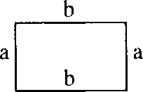
The perimeter is given by P = 2a + 2b and as the length of the fence is 400 m we get:
![]()
We wish to find the maximum area, and to do this we need to be able to differentiate A in terms of one of the variables, a or b. We use the information given about the length of the perimeter to express a in terms of b;
![]()
and substitute this into the expression for the area, giving
![]()
To find the maximum value for A differentiate with respect to b:

and solve

Check that this is indeed a local maximum value by differentiating a second time: d2A/db2 = −2, which is negative.
Now we find the length of the other side of the field
![]()
Therefore, the field with maximum area is a square of side 100. The area of the field is 100 × 100 = 10 000 m2.
To check that this agrees with the original condition that 2a + 2b = 400, substitute a = 100 and b = 100 to get 200 + 200 = 400, which is correct.
11.3 Graph sketching by analysing the function behaviour
To sketch the graph of any function y = f (x), we first analyse the main features of the function's behaviour. Look at the graph in Figure 11.7 and list the ‘important features’ of the graph. List these in a way that would enable someone else to sketch the graph from your description.

Here are some of the important features. The list is not exhaustive but should be enough to enable someone to reproduce the graph:
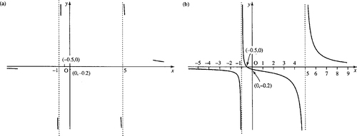
1. The graph is positive for x < −2 and x > 3 and negative for x between –2 and +3. There are no values of x for which y is zero and when x = 0, y = −0.167.
2. The graph is discontinuous at x = −2 and x = 3. y keeps getting larger as x approaches −2 from the left. A more precise way of expressing this is to say that as x tends to −2, with x less than −2, y tends to infinity. The symbol for infinity is ∞ and the symbol for ‘tends to’ is →. x tends to −2, with x less than −2 can be expressed more briefly as x → 2−. This gives
![]()
Similarly
![]()
For the discontinuity at x = 3 we have:
![]()
![]()
3. There is a local maximum at x = 0.5, where y = −0.16.
4. For large values of x, y gets nearer to 0. This can be expressed as
![]()
Similarly:
![]()
This list of important features indicates the steps that should be taken in order to sketch a graph:
Step 1. Find the value of y when the graph crosses the y-axis; that is, when x = 0. If possible find where the graph crosses the x-axis; that is, the values of x where y = 0.
Step 2. Find any discontinuities in the function, that is, are there values of x where there is no value of y? Infinite discontinuities (a ‘divide by zero’) will lead to vertical asymptotes. These are vertical lines which the function approaches but does not meet. We must decide whether the function is positive or negative on either side of the asymptote.
Step 3. Find the co-ordinates of the maxima and minima.
Step 4. Find the behaviour of the function as x tends to plus and minus infinity.
Step 5. Mark these features, found from steps 1 to 4 on the graph and join them, where appropriate, to give the sketch of the graph.
Example 11.6
Sketch the curve whose equation is

Solution
Step 1. When x = 0:
When y = 0,

then 2x + 1 = 0 ⇔ x = −0.5
Step 2. If the bottom line of the function were 0 this would lead to a ‘divide by zero’ which is undefined. This happens when x + 1 = 0, that is, x = −1 and when x – 5 = 0, that is, x = 5.
These are infinite discontinuities, that is, y will tend to plus or minus infinity as x approaches these values. The lines at x = – 1 and x = 5 are the asymptotes.
To find the sign of y on either side of the asymptotes substitute values of x on either side of them (avoiding including any values where y = 0). This can be done using a table, as in Table 11.1.
Table 11.1
Finding the sign on either side of the asymptotes
| x | −2 | −1 | −0.75 | −0.5 | 4 | 5 | 6 |
| y = 2x + 1/[(x + 1)(x − 5)] | −0.4286 | Not defined | 0.348 | 0 | −1.8 | Not defined | 0.93 |
| Sign of y | − | Not defined | + | 0 | − | Not defined | + |
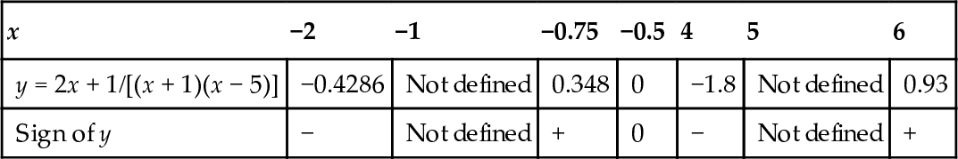
Using Table 11.1, we can conclude that as y is negative to the left of the asymptote at x = – 1 and positive to the right, then

Similarly, as y is negative to the left of the asymptote at x = 5 and positive to the right of it, then

Step 3. To find the turning points look for points where dy / dx = 0
To differentiate, first multiply out the brackets on the bottom line of the expression and then use the formula for finding the derivative of a quotient.
This gives

We now solve dy/dx = 0

Using the formula to solve the quadratic equation gives

Because of the square root of a negative number in this expression we can see that there are no real solutions; here, there are no turning points.
Step 4. When x is large in magnitude then the highest powers of x on the top and bottom lines of the function expression will dominate. In this case ignore all the other terms. Considering

For x large in magnitude
![]()
which tends to 0 and is positive as x → ∞ and tends to 0 and is negative as x → – ∞. We can say that as x → ∞, y → 0+ and as x → – ∞, y → 0−.
Step 5. Sketch the graph. This is done in two stages, as shown in Figure 11.8.
Example 11.7
A spring of modulus of elasticity k has a mass, m, suspended from it and is subjected to a oscillating force F = F0 cos(ωt), where ω > 0. The motion of the mass is damped by the use of a dashpot of damping constant c. This is displayed in Figure 11.9. After some time the spring force is found to have oscillations of angular frequency ω and of magnitude

Taking m = 1 and k = 1, sketch the graph of F / F0against ω for
![]()
Solution We are given that

Therefore,

Substituting m = 1 and k = 1 gives
Call this function H.
One method to solve this problem would be to consider cases (a), (b), (c), and (d) separately. However, it is quicker to leave c as an unknown constant and substitute in for the particular cases later.
Step 1.
when ω = 0, H = 1. The denominator is a positive square root, which means that H is always ≥ 0 where it is defined.
Step 2. Consider any points where H is not defined

As the term inside the square root in the expression for H is a sum of squares it is always, ≥ 0. This means that H is always defined, except where the denominator is 0. H is not defined when

By substituting the values of c of interest we see that in case (a) when c = 2, in case (b) when c = 1/2, and in case (c) when c = 1/4 there are no real solutions of this equation for ω. This means that there are no points where H is undefined. However, for case (d), where c = 0 we get the equation

As the frequency of the forcing function is positive then we just have the one value where H is discontinuous, at ω = 1. For case (d), where c = 0, H is undefined when ω = 1. This is an infinite ‘divide by zero’ discontinuity. We have already noted that H is always positive where it is defined and so we know that as ω → 1−,H → +∞ and as ω → l+,H → + ∞.
Step 3. To find the stationary points solve dH/dω = 0

is easier to differentiate if we use the rules of powers to give
![]()
Using the function of a function rule we get
Dividing the top and bottom lines by 2 and rearranging the terms on the top line gives
Setting dH/dω = 0 gives

multiplying both sides by – 1 times the denominator of the left-hand side gives

As we assume that the frequency is positive (or zero) there are two possibilities and ω = 0 and ![]() . The second case does not give a real solution if c = 2.
. The second case does not give a real solution if c = 2.
We wait until specific values of c are substituted in order to analyse the type of stationary points and the value of H at these points. Also note that this analysis is not valid for the case c = 0 as this completely changes the nature of the function H.
Step 4. When ω is large in magnitude
![]()
and this tends to 0 for large ω. Therefore, as ω → ∞, H → 0+.
Step 5. Now we can sketch the graph using the information found and after substituting the various values of c.
Case (a): c = 2. On substituting c = 2, we have

The graph passes through (0, 1) (Step 1), and the function is defined for all ω ≥ 0 (Step 2). The stationary point is at ω = 0. In this case
This is positive for ω < 0 and negative for ω > 0 and therefore there is a maximum value at ω= 0.
Case (b): ![]() . Here
. Here
The graph passes through (0, 1) (Step 1), and there are no discontinuities (Step 2). The stationary points are at ω = 0 and ![]() (Step 3):
(Step 3):
dH/dω< 0 for ω < 0 and dH/dω> 0 for ω > 0; therefore, there is a minimum value at ω = 0,
dH/dω > 0 for ω just less than ![]() ,
,
dH/dω < 0 for ω just greater than ![]() .
.
Therefore there is a maximum value of H at ![]()
At the maximum
![]()
Case (c): ![]()

The graph passes through (0, 1) (Step 1) and there are no discontinuities (Step 2). The stationary points are at ω = 0 and ![]() . There is a minimum value at ω = 0 and a maximum at
. There is a minimum value at ω = 0 and a maximum at ![]() where
where

Case (d): c = 0

The graph passes through (0, 1) (Step 1). There is an infinite discontinuity at ω = 1, and for

The stationary points have to be analysed separately as the general case always assumed c > 0. Differentiating H we get
which has a zero value at ω = 0.
dH/dω is negative for ω just less than 0 and positive for ω just greater than 0. Therefore, there is a minimum point at ω = 0. We can now sketch the graphs as in Figure 11.10.
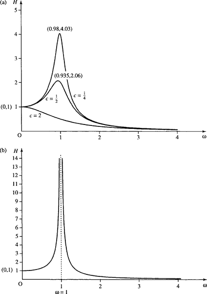
 , as in Example 11.7 for c = 2, c =
  , and c =
  . (b) The graph of H for c = 0. H = 1/(1−ω2) tor ω < 1 and H = 1/(ω2 – 1) for ω > 1.
11.4 Summary
1. To find and classify stationary values of a function y = f (x), then
Step 1. find dy/dx and solve for x such that dy/dx = 0
Step 2. classify the stationary points.
Method 1. By examining the sign of dy/dx near the point, in which case + → 0 → – indicates a local maximum point, – → 0 → + indicates a local minimum point, and + → 0 → + or – → 0 → – indicates a point of inflexion.
Method 2. By finding d2y/dx2at the point.
If d2y/dx2< 0 then there is a local maximum point
If d2y/dx2> 0 then there is a local minimum point
However, if d2y/dx2= 0 then this test is inconclusive and Method 1 must be used instead.
Substitute the values of x at the stationary points to find the relevant values of y. Local maxima and minima are also called turning points.
2 If the function, defined for a range of values of x, is continuous, then the overall maximum and minimum values can be found by finding the values of y at the local maxima and minima and the values of y at the boundary points. The maximum of all of these is the global maximum and the minimum of all of these is the global minimum value.
3 There are many practical problems that involve the need to find the maximum or minimum value of a function.
4 The stationary values are used when sketching a graph. We also look for:
(a) values where the graph crosses the axes;
(b) points of discontinuity and the behaviour near discontinuities;
(c) behaviour as tends to ±∞.
11.5 Exercises
11.1. Find and classify the stationary points of the following functions:
(b) y = −3x2 + 4x
(c) y = 3x3 − x
(d) ![]()
(e) w = z4 + 4z3 – 8z2 + 2
11.2 Find the overall maximum and minimum value of x/(2x2+ 1) in the range x ∈ [−1,1]
11.3. Sketch the graphs of the following functions:
(b) ![]()
(c) y = x3 – 3x − 1
(d) ![]()
11.4. Sketch the graph of y = 2 sin(x) – sin(2x) for x between – 2π and 2π.
11.5. Find the overall maximum and minimum value of y = x3(x −1) in the range x ∈ [0,2].
11.6. An open box of variable height and width is to have a length of 3 m. It should not use more than a total of 20 m 2 of surface area. Find the height and width that gives maximum volume.
11.7. An LRC series circuit has an impedance of magnitude
where R is the resistance, L the inductance, C the capacitance and ωis the angular frequency of the voltage source. Sketch Z against ω for the case where R = 200 Ω, C = 0.03 µF L = 2mH.
11.8. A crank is used to drive a piston as in Figure 11.11. The angular velocity of the crank shaft is the rate of change of the angle θ ω = dθ/dt. The piston moves horizontally with velocity υp and acceleration ap. The crankpin performs circular motion with a velocity of υcand centripetal acceleration of ω2r. The acceleration ap of the piston varies with θ and is related by

where r is the length of the crank and l is the length of the connecting rod. Substituting r = 150 mm and l = 375 mm find the maximum and minimum values of the acceleration ap.

11.9. A water wheel is constructed with symmetrical curved vanes of angle of curvature θ. Assuming that friction can be taken as negligible, the efficiency, η, that is, the ratio of output power to input power, is calculated as

where V is the velocity of the jet of water as it strikes the vane, υ is the velocity of the vane in the direction of the jet, and θ is constant. Find the ratio υ/V that gives maximum efficiency and find the maximum efficiency.
11.10. Power is transmitted by a fluid of density ρ moving with positive velocity V along a pipeline of constant cross-section areaA.Assuming that the loss of power is mainly attributable to friction and that the friction coefficient f can be taken to be a constant, then the power transmitted is given by P, P = pg A(h V – c V3), where, g is acceleration due to gravity and h is the head (the energy per unit weight). c = 4 f l/2gd where l is the length of the pipe and d is the diameter of the pipe. Assuming h is a constant find the value of V which gives a maximum value for P, and given the input power is Pi = pg A V h, find the maximum efficiency.