Search in book...
Toggle Font Controls
Create new playlist

Name your new playlist

Playlist description (optional)
Sign In

Email address

Password

Forgot Password?

or

Continue with Facebook

Continue with Google
Sign Up

Full Name

Email address

Confirm Email Address

Password

or

Continue with Facebook

Continue with Google

Differential equations and difference equations

14.1 Introduction

In order to model most physical situations we need to simplify their description. The idea of a system is central to this simplification. We identify the important elements that interact within the system. The only external interactions characterized as system inputs and the outputs are the quantities related to the system behaviour which we are interested in measuring. For instance, in examining the suspension system of a car we consider the system input to be forces exerted on the wheels of the car. The important elements in the system are the mass of the car and the springs and dampers used to connect the body of the car to the suspension links. We are interested in measuring the amount of vertical movement of the car and the velocity of that movement in response, mainly, to a bumpy road. We can examine the behaviour of the system for various external forces – building up a picture of how the system behaves in normal driving conditions. We do not need to concern ourselves with an exact model of the surface of the major motorways. In this way we have managed to separate the problem of modelling the system from modelling the environment in which it is operating. A system with a single input and output is pictured in Figure 14.1.

f14-01-9780750658553 — Figure 14.1 A system has an input f(t) which produces an output response y(t).

Dynamic physical processes involve variables which are interdependent and constantly changing. When modelling the system we will obtain relationships between variables, many of which will be related through derivatives. Even in a simple system with a mass, spring, and damper, there are many variables which can be identified, for example the extension of the spring, and its velocity and acceleration, the potential energy stored in the spring and the force exerted by it, and the force exerted by the damper. A choice of variables that completely describe the system is an important task in systems analysis. These variables are then called the state variables. These can be related to each other and the system inputs through a system of first-order differential equations which are found by using scientific laws and engineering principles to model the system. The system output, which is some quantity that we wish to compare with the response of a real system, can then be calculated from the values of the state variables.

A differential equation is one that involves some derivatives of the dependent variable, for example, dy/dt = ky is a differential equation. We have already looked at a number of examples of differential equations. The simplest case, when the solution can be found by integration, was looked at in Chapter 7 and then we found that exponential functions are solutions to differential equations of the form dy/dt = ky in Chapter 8 and in Chapter 10 we looked at the problem of circular motion and found that exponential functions are also solutions to equations of the form d²y/dt² = −ω²y. In simple equations, we look for a solution which is a number. When solving a differential equation our idea of a solution is to find an explicit function for y in terms of t.

We will only be concerned with single input, single output (SISO) systems in which case there are two ways of proceeding in order to solve the system of differential equations. The system may be reduced to a single differential equation and then solved, or the system may be solved directly. These two methods correspond, in systems theory, to the transfer function description of the system or a state variable description.

The types of differential equations we shall look at are all linear; that is, they involve no powers of y, the independent variable or powers of the derivative or products of any of these. Any real system will, of course have some non-linear behaviour. However, we usually assume that either the non-linearities present are not very important or that it is possible to analyse a system as locally linear. Another important assumption used is that time invariance, that is, operating the system now or in an hours time with exactly the same input and initial conditions will yield the same result.

The method of solution we use for finding a particular solution of differential equations in this chapter is called the method of unknown coefficients. An alternative method, using Laplace transforms, is more widely applied, and we shall look at them in the next chapter.

Differential equations are used to analyse systems that are subject to continuous or piecewise continuous inputs. It may be necessary, or preferable, to develop a discrete model of the system. A discrete model may be used if the exact nature of the system is unknown and we attempt to predict its nature by recording its response to various inputs. The recording of the system inputs and response will generally be stored in digital form and the data processed in digital form. Another major application of digital systems is for digital filter design. Here we wish to design digital filters with certain desirable characteristics. We can find the characteristics of digital systems by solving difference equations. We give a method of solution of simple difference equations. More frequently, z-transforms are used and these are discussed in the next chapter.

14.2 Modelling simple systems

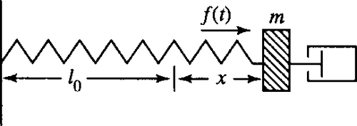
Damped forced motion of a spring

A spring of length l has a mass m attached to it and a dashpot damping the motion. It is subject to a force f(t) forcing the motion (see Figure 14.2).

f14-02-9780750658553 — Figure 14.2 Damped forced motion of a spring.

The input to this system is the forcing function f(t) and the output is the displacement of the spring from its original length, x. In order to model this system we make a number of assumptions about its behaviour.

1. We assume Newton's second law, F_T = ma where a = m d²x/dt² and F_T is the total force operating on the mass: m is the mass on the spring.

2. The spring does not become distorted, that is, it is perfectly elastic. This means, from Hooke's Law, that F_S = −kx where x is the displacement from the original spring length l and k is the spring constant.

3. The damping force due to the dashpot is F_D = −r dx/dt

To relate these quantities together we use the fact that the total force on the mass is made up of the spring force, the damping force, and the external force F_T = F_D + F_S + f(t).

If we wish to combine these equations to express them using a single differential equation we simply substitute for F_T in terms of x and the derivatives of x, giving

$\begin{array}{l} m \frac{d^{2} x}{d t^{2}} = - r \frac{d x}{d t} - k x + f (t) \\ ? ? ? ? \Leftrightarrow ? ? m \frac{d^{2} x}{d t^{2}} + r \frac{d x}{d t} + k x = f (t) \end{array}$

si1_e

Should we wish to solve the system as a system of first order differential equations then we choose some state variables, usually the displacement and the velocity. Called these x₁ and x₂, and as x₁ is the displacement x₁ = x and as x₂ is the velocity this is the derivative of the displacement giving x₂ = dx₁/dt.

As the acceleration is the derivative of the velocity, we can write the acceleration as the derivative of x₂

$a = \frac{d^{2} x_{1}}{d t^{2}} = \frac{d}{d t} \frac{d x_{1}}{d t} = \frac{d x_{2}}{d t} .$

si2_e

Now F_T = ma can be written in terms of x₂ as F_T = m dx₂/dt and the force due to the dashpot becomes F_D = −rx₂. So F_T = F_D + F_S + f(t) gives

$\begin{array}{l} m \frac{d x_{2}}{d t} = - r x_{2} - k x_{1} + f (t) \\ ? ? ? \Leftrightarrow ? ? \frac{d x_{2}}{d t} = - \frac{k}{m} x_{1} - \frac{r}{m} x_{2} + \frac{1}{m} f (t) . \end{array}$

si3_e

So the system of equations that represent the system is

$\begin{array}{l} \frac{d x_{1}}{d t} = x_{2} \\ \frac{d x_{2}}{d t} = - \frac{k}{m} x_{1} - \frac{r}{m} x_{2} + \frac{1}{m} f (t) . \end{array}$

si4_e

The first equation expresses the fact that x₂ is the velocity and the second equation was obtained by considering the total force on the mass and using Newton's second law.

This system of equations may be expressed in matrix form as

$\frac{d}{d t} (_{x_{2}}^{x_{1}}) = (?_{- k / m}^{0} ? ? ?_{- r / m}^{1}) (?_{x_{2}}^{x_{1}}) + (?_{1 / m}^{0}) ? f (t) .$

si5_e

Writing

$\begin{array}{l} x = (?_{x_{2}}^{x_{1}}) \\ A ? = (?_{- k / m}^{0} ? ? ?_{- r / m}^{1}) \end{array}$

si6_e

and

$B ? = (?_{1 / m}^{0})$

we can give the system of equations as a matrix differential equation

$\frac{d x}{d t} = A x + B f .$

si8_e

The system input is f and the output y = x₁.

To write the derivative of a variable when it is clear that it is in respect to its independent variable we may write x’ (read as ‘x dashed’) or x″ (read as ‘x double dashed’). In addition, when the independent variable is time we often write $\dot{x}$ (read as ‘x dot’) and for the second derivative x (read as ‘x double dot’). Using this notation we have

$\dot{x} = A x + B f$

as the matrix differential equation.

Modelling electrical circuits

We can model an LRC circuit as shown in Figure 14.3 using the following assumptions:

f14-03-9780750658553 — Figure 14.3 An LRC circuit.

1. Kirchoff's voltage law (KVL): the sum of all the voltage drops around any closed loop is zero.

2. The voltage drop v_R across a resistor is proportional to the current i i.e.

$ν_{R} = R i ? ? ? (O h m' s ? l a w)$

where the constant of proportionality R is called the resistance of the resistor.

3. The voltage drop across a capacitor is proportional to the electric charge q on the capacitor

$ν_{c} = \frac{1}{C} q$

si12_e

where C is the capacitance and is measured in farads, the charge q is measured in coulombs.

4. The voltage drop across an inductor is proportional to the rate of change of the current i

$ν_{L} = L \frac{d_{i}}{d t}$

si13_e

where L is the inductance, measured in henries.

Then, from KVL:

$L \frac{d i}{d t} + R i + \frac{q}{C} = v (t)$

si14_e

Since

$i (t) = \frac{d q}{d t}$

si15_e

we have

$\frac{d i}{d t} = \frac{d}{d t} (\frac{d q}{d t}) = \frac{d^{2} q}{d t^{2}}$

si16_e

So we can write this differential equation in terms of q:

$L \frac{d^{2} q}{d t^{2}} + R \frac{d q}{d t} + \frac{q}{C} = v (t) .$

si17_e

Here, the system input is v and the output is the charge on the capacitor q.

To obtain a differential equation in terms of i we can differentiate the whole of this equation and use i = dq/dt, giving

$L \frac{d^{2} i}{d t^{2}} + R \frac{d i}{d t} + \frac{i}{C} = \frac{d v}{d t} .$

Here the input is dv/dt and the output is i. Notice that L, R, and 1/C are constants.

Should we wish to solve the system as a system of first order differential equations then we choose some state variables. The general procedure is to choose capacitor voltages and inductor currents. Hence, we choose

x₁ = i

and

x₂ = υ_c = q/C.

We can obtain one equation relating x₁ and x₂ by using

$\frac{d q}{d t} = i ? ? \frac{1}{C} \frac{d q}{d t} = \frac{i}{C} ? ? \frac{d x_{2}}{d t} = \frac{x_{1}}{C} .$

si19_e

Now we use KVL to give the other equation

$L \frac{d i}{d t} + R i + \frac{q}{C} = v (t)$

si20_e

substituting i = x₁ and x₂ = q/C gives

$\frac{d x_{1}}{d t} = - \frac{R}{L} x_{1} - \frac{1}{L} x_{2} + \frac{1}{L} v (t) .$

si21_e

So the system of equations that give the state variables are

$\begin{array}{l} \frac{d x_{1}}{d t} = - \frac{R}{L} x_{1} - \frac{1}{L} x_{2} + \frac{1}{L} v (t) \\ \frac{d x_{2}}{d t} = \frac{1}{C} x_{1} . \end{array}$

si22_e

The first equation expresses Kirchoff's voltage law the second equation expresses the relationship between the current and the voltage across the capacitor.

This system of equations may be expressed in matrix form as

$\frac{d}{d t} (? \begin{matrix} x_{1} \\ x_{2} \end{matrix}) = (\begin{matrix} - R / L & - 1 / L \\ 1 / C & 0 \end{matrix}) ? (\begin{matrix} x_{1} \\ x_{2} \end{matrix}) + (\begin{matrix} 1 / L \\ 0 \end{matrix}) v .$

si23_e

Writing

$\begin{array}{l} x = (\begin{matrix} x_{1} \\ x_{2} \end{matrix}) \\ A = (\begin{matrix} - R / L & - 1 / L \\ 1 / C & 0 \end{matrix}) \end{array}$

si24_e

and

$B ? = (\begin{matrix} 1 / L \\ 0 \end{matrix})$

si25_e

This can be written as a matrix differential equation

$\frac{d x}{d t} = ? A x ? + ? B v .$

A rotational mechanical system

A rotor of moment of inertia J is supported by a shaft of torsional stiffness k and the motion is damped by a rotational damper of torque c per unit angular velocity (see Figure 14.4). T is the external torque applied to the rotor.

f14-04-9780750658553 — Figure 14.4 A damped rotational system.

The torque due to the rotational spring is proportional to the angle through which it has been twisted, giving T_S = −kθ. The damper provides a torque of −cω and the total rotational torque of the system is given by J dω/dt where ω is the angular velocity and J is the moment of inertial of the rotating body.

$\begin{matrix} J \frac{d ω}{d t} = - c ω - k θ + T \\ J \frac{d ω}{d t} + c ω + k θ = T . \end{matrix}$

si27_e

Using ω = dθ/dt, we can write this equation in terms of the angle of rotation as

$J \frac{d^{2} θ}{d t^{2}} + c \frac{d θ}{d t} + k θ = T$

Alternatively, we can choose state variables as x_l = θ and x₂ = ω = dx₁/dt. This gives the system of equations

$\frac{d}{d t} (? \begin{matrix} x_{1} \\ x_{2} \end{matrix}) ? = ? (\begin{matrix} 0 & 1 \\ - k / J & - c / J \end{matrix}) ? (\begin{matrix} x_{1} \\ x_{2} \end{matrix}) ? + ? (\begin{matrix} 0 \\ 1 / J \end{matrix}) ? T .$

Initial conditions and boundary values

To solve these equations we also need knowledge of the state of the system at some moment or moments in time. This is usually given in terms of the initial displacement and the initial velocity, that is, x and dx/dt at t = 0. This is then called an initial value problem. If two values of the displacement are given at different times or if the velocity and the displacement are given at different times, then the problem is called a boundary value problem. Boundary value problems are more difficult to specify correctly to ensure that they determine a solution.

14.3 Ordinary differential equations

An ordinary differential equation is an equation which involves derivatives of y (the dependent variable) as well as functions of y and t.

$\begin{array}{l} \frac{d y}{d t} = cos (t) \\ \frac{d^{2} y}{d t^{2}} + 9 t = 0 \\ t^{2} \frac{d^{3} y ? d y}{d t^{3} d t} + e^{t} = t \end{array}$

si30_e

are all ordinary differential equations.

The other sort of differential equations, which are introduced in Chapter 17, are partial differential equations which are used to describe a dependency on two independent variables and involve partial derivatives like ∂y/∂t (read as ‘partial dy by dt′).

The order of differential equations

The order of the differential equation is the order of the highest derivative of y (the dependent variable) in the equation.

$\begin{array}{l} R \frac{d q}{d t} + \frac{q}{C} = 3 & is ? first ? order ? in ? q . \\ \frac{d θ}{d t} = sin (θ) & is ? first ? order ? in ? θ . \\ x^{″} + 4 t^{2} = 0 & is ? second ? order ? in ? x . \\ \frac{d^{3} u}{d t^{3}} - \frac{d u}{d t} + u = 4 t^{4} & is ? third ? order ? in ? u . \end{array}$

si31_e

The solution of a differential equation

If a function, y = g(t), is a solution to a differential equation in y then if, in the differential equation, we replace y and by g(t) and all the derivatives of y by the corresponding derivatives of g(t) then the resulting predicate should be an identity for t. That is, it should be true for all values of t where it is defined.

Example 14.1

Show that x = t³ is a solution to the differential equation dx/dt = 3t².

Solution Replace x by t³ in the differential equation gives

$\frac{d}{d t} (t^{3}) = 3 t^{2}$

si32_e

$\Leftrightarrow ? ? ? ? 3 t^{2} = 3 t^{2}$

As this is true for all values of t, we have shown that x = t³ is a solution to dx /dt = 3t².

Example 14.2

Show that y = t² – 3t + 3.5 is a solution to

$y ″ + 3 y' + 2 y = 2 t^{2} .$

Solution Set y = t² – 3t + 3.5, then differentiating gives

$y' = 2 t - 3$

and differentiating again

$y ″ = 2$

We substitute these expressions for y and the derivatives of y into

$y ″ + 3 y' + 2 y = 2 t^{2}$

so we get

$\begin{matrix} 2 + 3 (2 t - 3) + 2 (t^{2} - 3 t + 3.5) = 2 t^{2} \\ \begin{array}{l} \Leftrightarrow ? ? 2 + 6 t - 9 + 2 t^{2} - 6 t + 7 = 2 t^{2} \\ \Leftrightarrow ? ? 2 t^{2} = 2 t^{2} \end{array} \end{matrix}$

si38_e

which is true for all values of t showing that y = t² – 3t + 3.5 is a solution to y″ + 3y′ + 2y = 2t².

A differential equation has many solutions. For instance, the equation dx/dt = 3t² has solutions x = t³, x = t³+ 4, x = t³ – 5, etc. These are called particular solutions. A general solution is one which contains some arbitrary constants and encompasses all possible solutions to the differential equation. This means that by choosing values of these arbitrary constants we are able to find any of the particular solutions of the equation. For instance, x = t³ + C is a general solution to dx/dt = 3t².

Linear differential equations

A linear differential equation can be recognized by its form. It is linear if the coefficients of y (the dependent variable) and all order derivatives of y, are functions of t, or constant terms, only.

$\begin{array}{l} d y / d t = 4 t \\ d^{2} y / d t^{2} = 6 t \\ t ? d y / d t = 6 \\ a y ″ + b y' + c y = f (t) \\ 3 d^{2} y / d t^{2} + t^{2} d y / d t + 6 y = t^{5} \end{array}$

si39_e

are all linear.

$\begin{array}{l} {(d y / d t)}^{2} + 3 = 12 t + y ? d y / d t - t^{2} \\ θ ″ + k ? sin (θ) = 0 \\ u ″ - (1 - u^{2}) u' + u = 0 \end{array}$

si40_e

are all non-linear.

Linearity and superposition of solutions

The property of linearity is very important. We have applied the term linear to equations whose graphs are straight lines. However, in an algebraic sense the term does not mean that everything represents a straight line! The property of linearity is defined for an operator, which we shall call O. A linear operator is one that, when operating on the sum of two terms gives the same result as operating on the terms and then taking the sum. This can be expressed as

$O (f_{1} + f_{2}) = O (f_{1}) + O (f_{2}) .$

The other condition is that

$O (a f) = a O (f)$

The two conditions can be combined to say that a linear operation on a linear combination of inputs produces a linear combination of the outputs. A linear combination of f₁ and f₂ is af₁ + bf₂, where a and b are constants and therefore if an operator, O, is linear then

$O (a f_{1} + b f_{2}) = a O (f_{1}) + b O (f_{2})$

Examples of linear operators are:

Matrices

A(x₁ + x₂) = Ax₁ + Ax₂ and A(ax) = a(Ax) where a is a number and A is a matrix and x₁, X₂, and x are vectors

The differential operator

$\frac{d}{d t} (3 t + t^{2}) = 3 \frac{d}{d t} (t) + \frac{d}{d t} (t^{2}) .$

si44_e

The integral operator

$\int (3 t + t^{2}) d t = \int 3 t ? ? d t + \int t^{2} ? ? d t$

An example of a non-linear operator is the sine function as

$sin (A + B) \neq sin (A) + sin (B)$

For a differential equation the fact that it is linear leads to the fact that if a solution to the differential equation with input function f₁(t) is y₁ and a solution to the differential equation with input f₂(t) is y₂, then one solution to the equation with an input function af₁ + bf₂ is ay₁ + by₂, where a and b are constants. This result is central to the method of solving differential equations used in this chapter and also to the Laplace transform method of the next chapter.

Example 14.3

A differential equation

$d^{2} x / d t^{2} + 9 x = f (t)$

is found to have a particular solution x = t /9 when f(t) = t and a particular solution

$\frac{1}{5} sin (2 t) ? ? ? ? ? when ? f (t) = sin (2 t) .$

si48_e

Suggest a particular solution when f(t) = t + 5 sin(2t) and check that your hypothesis is correct.

Solution As the differential equation is linear, if we sum the input functions then we should be able to sum the solutions. Hence, a solution to

$d^{2} x / d t^{2} + 9 x = t + 5 ? sin (2 t)$

should be given by

$x = \frac{t}{9} + 5 \times \frac{1}{5} sin (2 t) = \frac{t}{9} + sin (2 t)$

si50_e

Check:

$\begin{array}{l} x = t / 9 + sin (2 t) \\ d x / d t = (1 / 9) + 2 ? cos (2 t) \\ d^{2} x / d t^{2} = - 4 sin (2 t) \end{array}$

si51_e

Then substituting these into

$d^{2} x / d t^{2} + 9 x = t + 5 sin (2 t)$

gives

$\begin{array}{l} - 4 sin (2 t) + 9 ((t / 9) + sin (2 t)) = t + 5 sin (2 t) \\ ? ? ? ? ? - 4 sin (2 t) + t + 9 sin (2 t) = t + 5 sin (2 t) \end{array}$

si53_e

which is true for all values of t, showing that

$x = (t / 9) + sin (2 t)$

is a solution to

$d^{2} x / d t^{2} + 9 x = t + 5 sin (2 t) .$

Linear equations with constant coefficients

A linear equation is said to have constant coefficients if the coefficients multiplying y and the derivatives of y (the dependent variable) are all constants, that is, do not involve functions of t.

$3 ? d^{2} y / d t^{2} + 2 ? d y / d t + 4 y = f (t)$

has constant coefficients

$t^{2} d^{2} y / d t^{2} + 3 t ? d y / d t + 4 y = f (t)$

does not have constant coefficients as t² and 3t are functions of time.

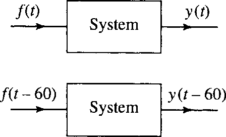
Time invariance

A linear differential equation with constant coefficients displays time invariance. If we use the same input and starting conditions for a system now or at some later time then the result relative to the initial starting time will be identical. Another way of expressing this is that if the input is time shifted then so is the output. This idea is represented in Figure 14.5.

f14-05-9780750658553 — Figure 14.5 If a system is time invariant, then a time-shifted input yields a time-shifted output.

Example 14.4

For the differential equation

$d^{2} y / d t^{2} + 4 y = sin (3 t)$

show that

$y = sin (2 t) - \frac{1}{5} sin (3 t)$

si59_e

is a solution and find a solution for the equation with the same input function delayed by 1 s, that is, find a solution to

$d^{2} y / d t^{2} + 4 y = sin (3 (t - 1))$

Solution First, we check that

$y = sin (2 t) - \frac{1}{5} sin (3 t)$

si61_e

is a solution to the differential equation.

To do this, we must find the first and second derivatives

$\begin{array}{l} d y / d t = 2 cos (2 t) - (3 / 5) cos (3 t) \\ d^{2} y / d t^{2} = - 4 sin (2 t) + (9 / 5) sin (3 t) \end{array}$

si62_e

Substitute into

$d^{2} y / d t^{2} + 4 y = sin (3 t)$

giving

$\begin{array}{l} - 4 sin (2 t) + (9 / 5) sin (3 t) + 4 (sin (2 t) - \frac{1}{5} sin (3 t)) = sin (3 t) \\ ? ? ? ? ? \Leftrightarrow ? ? ? sin (3 t) = sin (3 t) \end{array}$

si64_e

which is true for all t. Hence,

$y = sin (2 t) - \frac{1}{5} sin (3 t)$

si65_e

is a solution to

$d^{2} y / d t^{2} + 4 y = sin (3 t) .$

To find a solution to d²y/dt² +4y = sin(3(t −1)), we use the property of time invariance, which means that a solution should be given by a time-shifted version of the solution to the first equation, that is

$y = sin (2 (t - 1)) - \frac{1}{5} sin (3 (t - 1))$

si67_e

then

$\begin{array}{l} d y / d t = 2 cos (2 (t - 1)) - (3 / 5) cos (3 (t - 1)) \\ d^{2} y / d t^{2} = - 4 sin (2 (t - 1)) + (9 / 5) sin (3 (t - 1)) . \end{array}$

si68_e

Substitute into

$d^{2} y / d t^{2} + 4 y = sin (3 (t - 1))$

giving

$\begin{array}{l} - 4 sin (2 (t - 1)) + (9 / 5) sin (3 (t - 1)) \\ + 4 (sin (2 (t - 1)) - (1 / 5) sin (3 (t - 1))) \\ = sin (3 (t - 1)) \\ \Leftrightarrow ? ? ? ? sin (3 (t - 1)) = sin (3 (t - 1)) \end{array}$

si70_e

which is true for all t.

Example 14.5

For the differential equation

$t ? d y / d t + y = 6 t^{2}$

(a) show that y = 2t² is a solution

(b) show that the equation t dy/dt + y = 6t² cannot represent a time invariant system.

Solution (a) To show that y = 2t² is a solution to

$t ? d y / d t + y = 6 t^{2}$

we need to find dy/dt

$\begin{array}{l} y = 2 t^{2} \\ ? ? ? ? \Rightarrow d y / d t = 4 t \end{array}$

si73_e

substituting into

$t ? ? d y / d t + y = 6 t^{2}$

gives

$\begin{array}{l} t ? (4 t) + 2 t^{2} = 6 t^{2} \\ ? ? ? ? \Leftrightarrow ? ? ? ? ? 6 t^{2} = 6 t^{2}, ? which ? is ? true ? for ? all ? t . \end{array}$

si75_e

(b) To show that this cannot represent a time-invariant system, we take an equation with a time-shifted input, for instance, shifted by 2 s to give

$t ? ? d y / d t + y = 6 {(t - 2)}^{2} .$

If it were to be time-invariant, then a solution to this equation would be a time-shifted solution of the solution to the equation in part (a), that is, y = 2(t − 2)². To show that the equation does not represent a time-invariant system we just need to show that y = 2(t − 2)² is not a solution

$\begin{array}{l} y = 2 {(t - 2)}^{2} \\ ? ? ? ? \Rightarrow d y / d t = 4 (t - 2) \end{array}$

si77_e

Substitution into

$t ? d y / d t + y = 6 {(t - 2)}^{2}$

gives

$\begin{array}{l} t (4 (t - 2)) + 2 {(t - 2)}^{2} = 6 {(t - 2)}^{2} \\ ? ? ? ? \Leftrightarrow ? ? ? 4 t (t - 2) + 2 {(t - 2)}^{2} - 6 {(t - 2)}^{2} = 0 \\ ? ? ? ? \Leftrightarrow ? ? ? (t - 2) (4 t + 2 t (t - 2) - 6 (t - 2)) = 0 \\ ? ? ? ? \Leftrightarrow ? ? ? (t - 2) (4 t + 2 t - 4 - 6 t + 12) = 0 \\ ? ? ? ? \Leftrightarrow ? ? ? 8 (t - 2) = 0 \end{array}$

si79_e

which is not true for all values of t, showing that y = 2(t − 2)² is not a solution to t dy/dt + y = 6(t − 2)² and therefore we have shown that t dy/dt + y = f(t) does not represent a time-invariant system.

We have seen that linear differential equations with constant coefficients represent linear time invariant (LTI) systems.

14.4 Solving first-order LTI systems

To solve ay′ + by = f(t), we begin by ignoring the forcing function setting it equal to 0. This is then called the homogeneous equation

$a y' + b y = 0.$

The general solution to this equation is called the complementary function.

We then find any particular solution and the sum of the complementary function and the particular solution gives us the general solution to the differential equation. Summing the two solutions in this way we are making use of the linearity property of the differential equation.

It may seem strange that a system with no input, as represented by the homogeneous equation ay′ + by = 0 may have a non-zero output! This is due to the fact that the initial conditions may be non-zero. For instance, a pendulum released from rest and performing small oscillations, approximately obeys the differential equation

$d^{2} y / d t^{2} + ω^{2} y = 0$

where y is the distance the tip of pendulum has moved from its rest position and ω is its angular velocity. The pendulum will only begin to move if either it is given a non-zero initial velocity of if it is lifted slightly and then released. This means that either the initial position or the initial velocity or both must be non-zero for y to be non-zero.

The method we shall use for solving the complementary function relies on the fact that we know that y′ = ky has the solution y = C e^kt. That is, the derivative of an exponential function is a scaled version of the original function. This was discussed in Chapter 8. We can also show that any order derivative of an exponential function is a scaled version of the original function. Consider

$d y / d t = k y .$

Differentiating this equation gives

$d^{2} y / d t^{2} = k ? d y / d t .$

Substituting dy/dt = ky we get

$d^{2} y / d t^{2} = k^{2} y$

and hence the second derivative is a scaled version of the original exponential function with scaling factor k². Differentiating again, we get

$d^{3} y / d t^{3} = k^{2} d y / d t$

and on substituting dy/dt = ky, we get

$d^{3} y / d t^{3} = k^{3} y$

and hence the third derivative is a scaled version of the original function with scaling factor k³. We use this property of exponential functions to solve the homogeneous equation by trying a solution of the form y = C e^λt. We then find value(s) for λ which are appropriate for the equation under consideration.

The equations we found in Section 14.2 were all second-order equations or systems of equations involving more than one state variable. However, in some circumstances, we get simple first order equations. For instance if their is no inductor present in an LRC circuit we can put L = 0 to give

$R ? d q / d t + q / C = v (t),$

which is first order in q.

The method of solution can be characterized by four steps. To find the solution to ay′ + by = f (t):

Step 1: Find the complementary function

The solution of the homogeneous equation

$a y' + b y = 0$

is found by assuming a solution of the form y = A e^λt. Hence, y′ = Aλ e^λt and substituting into ay′ + by = 0 we get

$a ? A λ ? e^{λ t} + b A ? e^{λ t} = 0$

We are not interested in the trivial solution A = 0 and e^λt is never zero, so we can divide through by A e^λt giving

$λ a + b = 0$

which is called the auxiliary, or characteristic equation.

The auxiliary equation has the solution λ = –b/a. Hence, the complementary function is

$y = A ? e^{- (b / a) t} .$

Step 2: Find a particular solution

The system output, after the effect of any initial conditions have died out, we would expect to mimic the system input. To find a particular solution we try a trial solution with some undetermined coefficients. Some good guesses to use for the trial solution, depending on the type of input function f(t), are given in Table 14.1.

Table 14.1

A table of trial solutions to be used to find a particular solution. The form of the trial solution is suggested by the form of the forcing function f(t). The coefficients c₀, c_l,… and c,d are to be determined

Input function	Trial solution
Polynomial of order n
f(t) = a₀ + a₁t + a₂t² + ··· + a_ntⁿ	y = c₀ + c₁t + c₂t² + ··· + C_ntⁿ (Use all terms up to n for the trial solution)
Exponential function
f(t) = a e^αt	y = c e^αt
Sine or cosine function
f(t) = a cos(ωt) or b sin(ωt) or f(t) = a cos(ωt) + b sin(ωt)	y = c cos(ωt) + d sin(ωt)

The coefficients in the trial solution are determined by substituting into

$a y' + b y = f (t) .$

These trial solutions will not always work. Laplace transforms may be used to find a particular solution in that case (see Chapter 15).

Step 3: Find the general solution

The general solution to the equation is given by the sum of the complementary function plus the particular solution.

Step 4: Find the particular solution

The final step is to use the initial condition to find the appropriate value of A, the arbitrary constant. This solution is then the particular solution which solves the differential equation with the given initial condition.

Example 14.6

The RC circuit in Figure 14.6 is initially relaxed and is closed at time t = 0. Hence, applying a DC voltage of υ₀ the charge of the capacitor obeys the differential equation

$R ? d q / d t + q / C = v_{0} .$

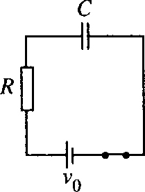
f14-06-9780750658553 — Figure 14.6 An RC circuit with an applied DC voltage.

Solve for q and find an expression for the voltage across the capacitor at a time t after the circuit was closed.

Step 1

To find the complementary function we solve the homogeneous equation

$R ? d q / d t + q / C = 0.$

Substitute q = A e^λt and dq/dt = Aλe^λt to give

$R λ A ? e^{λ t} + A ? e^{l t} / C = 0.$

Divide by A e^λt

$R λ + 1 / C = 0 ? ? ? ? \Leftrightarrow ? ? ? λ = - 1 / (R C) .$

The complementary function is

$q = A ? e^{- t / R C}$

Step 2

Try a particular solution of the form q = a, where a is a constant. Then q′ = 0, substituting into

$R ? d q / d t + q / C = v_{0}$

we get

$\begin{array}{l} a / C = v_{0} \\ ? ? ? ? \Leftrightarrow ? ? ? a = v_{0} C \end{array}$

si99_e

Step 3

The general solution is therefore the sum of the complementary function (found in Step 1) and a particular solution (found from Step 2), so the general solution for q is given by

$q = A ? e^{- t / R C} + C v_{0}$

Step 4

Finally, we use the initial conditions to find the arbitrary constant A. We are told that initially the circuit was relaxed meaning that all voltages and currents are zero. In this case, this means that when t = 0, q = 0. Substituting this condition into

$q = A ? e^{- t / R C} + C v_{0}$

we get

$\begin{array}{l} 0 = A + C ν_{0} \\ ? ? ? ? ? \Leftrightarrow ? ? A = - C ν_{0} \end{array}$

si102_e

Therefore, the solution is

$\begin{array}{l} q = - C ν_{0} ? e^{- t / R C} + C ν_{0} \\ ? ? ? ? \Leftrightarrow ? ? ? q = C ν_{0} (1 - e^{- t / R C}) . \end{array}$

si103_e

This gives the voltage across the capacitor v_c = q / C as v_c = v₀ × (1 – e ^−t^/^RC) where v₀ is the applied DC voltage.

Check:

To check that q = Cv₀(l – e^−t/^RC) is in fact a solution to

$R ? d q / d t + q / C = ν_{0}$

we carry out the following steps:

$\begin{array}{l} q = C v_{0} (1 - e^{- t / R C}) \\ ? ? ? ? \Rightarrow d q / d t = (C v_{0} / R C) e^{- t / R C} ? ? ? ? \Leftrightarrow ? ? ? ? ? d q / d t = (v_{0} / R) e^{- t / R C} \end{array}$

si105_e

Substituting into

$R ? d q / d t + q / C = v_{0}$

gives

$\begin{array}{l} (R v_{0} / R) e^{- t / R C} + (ν_{0} C / C) (1 - e^{- t / R C}) = ν_{0} \\ ? ? ? ? ? ? \Leftrightarrow ? ? ? ? ? ν_{0} = ν_{0} \end{array}$

si107_e

which is an identity for t, showing that q = Cv₀(1 – e ^−t^/RC) is a solution to the differential equation.

We also check that the solution satisfies the given initial condition by substituting q = 0 and t = 0 into q = Cv₀(1 – e^−t/RC). We find

$0 = C v_{0} (1 - 1) ? ? ? ? ? \Leftrightarrow ? ? ? ? ? 0 = 0,$

which is true.

Example 14.7

Solve the differential equation

$y' - 3 y = 6 cos (2 t),$

given y (0) = 2.

Step 1

To find the complementary function we solve the homogeneous equation

$y' - 3 y = 0$

substitute y = A e^λt so that dy = Aλ e^λt, giving

$A λ ? e^{λ t} - 3 A ? e^{λ t} = 0.$

Therefore, we get the auxiliary equation

$λ - 3 = 0 ? ? ? ? \Leftrightarrow ? ? ? ? λ = 3.$

The complementary function is y = A e^3t

Step 2

Try a particular solution (chosen from Table 14.1) of the form y = c cos(2t) + d sin(2t) then y′ = −2c sin(2t) + 2d cos(2t). Substituting into y′ − 3y = 6 cos(2t) we get

$\begin{array}{l} - 2 c ? sin (2 t) + 2 d ? cos (2 t) - 3 (c ? cos (2 t) + d ? sin (2 t)) = 6 ? cos (2 t) \\ ? ? ? \Leftrightarrow ? ? ? (- 2 c - 3 d) sin (2 t) + (2 d - 3 c) cos (2 t) = 6 ? cos (2 t) . \end{array}$

si113_e

We want this to be true for all values of t, so we can equate the coefficients of the sin(2t) terms on both sides of the equation and also the cos(2t) terms.

Equating the coefficients of sin(2t) gives:

$- 2 c - 3 d = 0.$

Equating the coefficients cos(2t) gives:

$- 2 d - 3 c = 6.$

Therefore,

$\begin{array}{l} - 2 c - 3 d = 0 \\ - 3 c + 2 d = 6. \end{array}$

si116_e

Solving these equations simultaneously gives

$c = - 18 / 13 ? ? ? ? d = 12 / 13.$

Hence, a particular solution is

$y = - (18 / 13) cos (2 t) + (12 / 13) sin (2 t) .$

Step 3

The general solution is given by the sum of the complementary function and a particular solution giving

$y = A ? e^{3 t} - (18 / 13) cos (2 t) + (12 / 13) sin (2 t) .$

Step 4

Use the initial condition to find A.

When t = 0, y = 2. Substituting this into

$y = A ? e^{3 t} - (18 / 13) cos (2 t) + (12 / 13) sin (2 t)$

gives

$\begin{array}{l} 2 = A - (18 / 13) cos (0) + (12 / 13) sin (0) \\ ? ? ? \Leftrightarrow ? ? ? 2 = A - 18 / 13 ? ? ? ? ? \Leftrightarrow ? ? ? A = 44 / 13. \end{array}$

si121_e

Therefore, the solution is

$y = (44 / 13) e^{3 t} - (18 / 13) cos (2 t) + (12 / 13) sin (2 t) .$

Check: Substitute

$y = (44 / 13) e^{3 t} - (18 / 13) cos (2 t) + (12 / 13) sin (2 t)$

and

$y' = (132 / 13) e^{3 t} + (36 / 13) sin (2 t) + (24 / 13) cos (2 t)$

into

$\begin{array}{l} y' - 3 y = 6 ? cos (2 t) ? giving \\ (132 / 13) e^{3 t} + (36 / 13) sin (2 t) + (24 / 13) cos (2 t) \\ ? ? ? - 3 (44 / 13) e^{3 t} - (18 / 13) cos (2 t) + (12 / 13) sin (2 t) = 6 cos (2 t) \\ ? ? ? ? \Leftrightarrow ? ? ? (78 / 13) cos (2 t) = 6 cos (2 t) \end{array}$

si125_e

which is correct.

We also check the initial condition by substituting t = 0, y = 2 into

$y = (44 / 13) e^{3 t} - (18 / 13) cos (2 t) + (12 / 13) sin (2 t) .$

We find

$\begin{array}{l} 2 = (44 / 13) e^{0} - (18 / 13) cos (0) + (12 / 13) sin (0) \\ ? ? ? \Leftrightarrow ? ? ? 2 = (44 / 13) - (18 / 13) \\ ? ? ? \Leftrightarrow ? ? ? 2 = 26 / 13, ? which ? is ? true . \end{array}$

si127_e

14.5 Solution of a second-order LTI systems

We can solve a second-order system in a manner similar to first-order systems. To solve ay″ + by′ + cy = f(t) we solve the homogeneous equation

$a y ″ + b y' + c y = 0.$

The solution to this equation is called the complementary function.

We then find any particular solution and the sum of the complementary function and a particular solution gives us the general solution to the differential equation. We can again list the steps involved.

$To ? solve ? a y^{″} + b y' + c y = f (t)$

Step 1 – Find the complementary function

The solution of the homogeneous equation

$a y ″ + b y' + c y = 0$

is found by assuming solutions of the form y = A e^λt. Hence, y′ = Aλ e^λt and v” = Aλ²e^λt and we find

$a A λ^{2} ? e^{t} + b A λ ? e^{λ t} + c A ? e^{λ t} = 0$

giving the auxiliary equation

$a λ^{2} + λ b + c = 0.$

The auxiliary equation is a quadratic equation. It has solutions

$λ_{1}, ? λ_{2} ? = ? \frac{- b \pm \sqrt{b^{2} - 4 a c}}{2 a} .$

si133_e

There are three possible types of solutions:

Case (1): λ_l and λ₂ are real and distinct then the solution is:

$y ? = ? A ? e^{λ_{1} t} + ? B ? e^{λ_{2} t} .$

Case (2): λ_l and λ₂ are complex. We set λ_l = k + jω₀ and λ₂ = k – jω₀

so that k = −b/2a and

$ω_{0} = \frac{\sqrt{4 a c - b^{2}}}{2 a} .$

si135_e

Then the complex exponentials can be written in terms of cosines and sines and the solution becomes

$y ? = ? e^{k t} (A ? cos (ω_{0} t) ? + ? B ? sin (ω_{0} t)) .$

Case (3): The roots are equal, that is, λ_l = λ₂ = k = −b/2a, then the solution is y = (At + B)e^kt.

Step 2: Find a particular solution

The particular solution is any solution of the equation

$a y ″ ? + ? b y' ? c y ? = ? f (t) .$

As for the first-order system we expect the system output, after the effect of any initial conditions have died out, to mimic the system input. Again to find a particular solution we try a trial solution as given in Table 14.1. The ‘guess’ at the particular solution is substituted into the differential equation and the unknowns coefficients can be determined. If this guess does not produce a solution then Laplace transform methods can be used as in Chapter 15.

Step 3

The general solution to the equation is given by the sum of the complementary function plus a particular solution.

Step 4

The final stage is to use the initial conditions or boundary conditions to find the appropriate values of the arbitrary constants A and B.

Example 14.8

Solve the differential equation 5y″ + 6y′ +5y = 6 cos(t), where y (0) = 0 and y′ (0) = 0.

Step 1

To find the complementary function we solve the homogeneous equation 5y″ + 6y′ + 5y = 0. Trying solutions of the form y = A e^λt leads to the auxiliary equation 5λ² + 6λ + 5 = 0. Notice that a quick way to get the auxiliary equation is to ‘replace’ y″ by λ², y′ by A, and y by 1. The auxiliary equation has solutions

$\begin{array}{l} λ & = & \frac{- 6 \pm \sqrt{36 - 100}}{10} \\ = & \frac{- 6 \pm \sqrt{- 64}}{10} \\ = & - 0.6 \pm j0 .8 . \end{array}$

si138_e

Comparing this with λ = k ± jω₀ gives k = −0.6, ω₀ = 0.8. This means that the complementary function has the form

$y ? = ? e^{k t} (A ? cos (ω_{0} t) ? + ? B ? sin (ω_{0} t))$

(given as Case (2) in the general method), with k = −0.6 and ω₀ = 0.8. This gives

$y ? = ? e^{- 0 .6 t} ? (A ? cos ? (0.8 t) ? + ? B ? sin (0.8 t)) .$

Step 2

As f(t) = 6 cos(t), from Table 14.1 we decide to try a particular solution of the form y = c cos(t) + d sin(t). Then

$y' ? = ? - c ? sin (t) ? + ? d ? cos (t)$

and

$y^{″} ? = ? - c ? cos (t) ? + ? d ? sin (t).$

Substituting in

$5 y^{″} ? + ? 6 y^{'} ? + ? 5 y ? = ? 6 ? cos (t)$

we find

$\begin{array}{l} 5 (- c ? cos (t) ? - ? d ? sin (t)) ? + ? 6 (- c ? sin (t) ? + ? d ? cos (t)) \\ ? ? ? ? ? ? + ? 5 ? (c ? cos (t) ? + ? d ? sin (t)) ? = ? 6 ? cos (t) \\ ? ? ? ? ? ? \Leftrightarrow ? ? ? ? ? ? (- 5 c ? + ? 6 d ? + ? 5 c) ? cos (t) ? + (- 5 d - 6 c + 5 d) ? sin (t) ? = ? 6 ? cos (t) \\ ? ? ? ? ? ? \Leftrightarrow ? ? ? ? ? ? ? 6 d ? cos (t) ? - 6 c ? sin (t) ? = ? 6 ? cos ? (t) . \end{array}$

si144_e

As we want this to be an identity we equate the coefficients of cos(t) and the coefficients of sin (t) and get the two equations

$\begin{array}{l} 6 d ? = ? 6 & \Leftrightarrow & d ? = ? 1 \\ 6 c ? = ? 0 & \Leftrightarrow & c ? = ? 0. \end{array}$

si145_e

Hence, a particular solution is y = sin(t).

Step 3

The general solution is given by the sum of the complementary function and a particular solution, so

$y ? = ? e^{- 0 .6 t} ? (A ? sin (0.8 t) ? ? + ? ? B ? cos (0.8 t)) ? + ? sin (t) .$

Step 4

Use the given initial conditions to find values for the constants A and B. Substituting y = 0 when t = 0 into

$y ? = ? e^{- 0 .6 t} ? (A ? cos (0.8 t) ? + ? B ? sin (0.8 t)) ? + ? sin (t)$

then

$\begin{array}{l} 0 & = & e^{0} (A ? cos (0) ? + ? B ? sin (0)) ? + ? sin (0) \\ \Leftrightarrow & 0 ? = ? A . \end{array}$

si148_e

To use the other condition, that y′ = 0 when t = 0, we need to differentiate the general solution to find an expression for y'. Differentiating (using the product rule):

$\begin{array}{l} y ? = ? e^{- 0 .6 t} ? (A ? cos (0.8 t) ? + ? B ? sin (0.8 t)) ? + ? sin (t) \\ ? ? ? ? ? ? ? \Rightarrow ? ? y^{'} ? = ? - 0.6 ? e^{- 0 .6t} ? (A ? cos (0.8 t) ? + ? B ? sin (0.8 t)) \\ ? ? ? ? ? ? ? + ? e^{- 0 .6 t} (- 0.8 A ? sin (0.8 t) ? + ? 0.8 ? B ? cos (0.8 t)) ? + ? cos (t) \end{array}$

si149_e

and using y′ = 0 when t = 0 gives

$0 ? = ? - 0.6 A ? + ? 0.8 B ? + ? 1.$

We have already found A = 0 from the first condition, so

$B ? = ? - 1 / (0.8) ? = ? - 1.25.$

Therefore, the solution is

$y ? = ? - 1.25 ? e^{- 0 .6 t} ? sin ? (0.8 t) ? + ? sin (t) .$

Check

$\begin{array}{l} y & = & - 1.25 ? e^{- 0 .6 t} ? sin ? (0.8 t) ? + ? sin (t) \\ y^{'} & = & 0.75 ? e^{- 0 .6 t} ? sin (0.8 t) ? - ? e^{- 0 .6 t} cos (0.8 t) ? +? cos (t) \\ y^{″} & = & - 0.45 ? e^{- 0 .6 t} ? sin (0.8 t) ? + ? 0.6 ? e^{- 0 .6 t} ? cos (0.8 t) \\ + ? 0.6 ? e^{- 0 .6 t} ? cos (0.8 t) ? + ? 0.8 ? e^{- 0 .6 t} ? sin ? (0.8 t) ? - ? sin (t) . \end{array}$

si153_e

Substitute into

$5 y^{″} ? + ? 6 ? y^{'} ? + ? 5 ? y ? = ? 6 ? cos (t)$

giving

$\begin{array}{l} 5 (- 0.45 ? e^{- 0.6 t} ? sin ? (0.8 t) ? + ? 0.6 ? e^{- 0 .6 t} ? cos (0.8 t) \\ ? ? ? ? ? + ? 0.6 ? e^{- 0 .6 t} ? cos (0.8 t) ? + ? 0.8 ? e^{- 0.6 t} ? ? sin ? (0.8 t) - sin (t)) \\ ? ? ? ? ? ? + ? 6 (0.75 ? e^{- 0.6 t} ? sin (0.8 t) ? - ? e^{- 0.6 t} ? cos (0.8 t) ? + ? cos (t)) \\ ? ? ? ? ? ? + ? 5 (- 1.25 ? e^{- 0.6 t} ? sin (0.8 t) ? + ? sin (t)) ? = ? 6 ? cos (t) \\ ? ? ? ? ? ? \Leftrightarrow ? ? ? ? ? ? e^{- 0.6 t} ? ? sin (0.8 t) ? (1.75 + 4.5 - 6.25) ? + ? e^{−0.6 t} ? cos (0.8 t) ? (6 - 6) \\ ? ? ? ? ? ? + ? ? ? sin (t) ? ? (- 5 + 5) ? + ? 6 ? cos ? (t) ? = ? 6 ? cos (t) \end{array}$

si155_e

which is true for all values of t.

We can also check that the solution satisfies the given initial conditions.

Example 14.9

Find the current in an initially relaxed LRC circuit with R = 5 Ω, L = 4 μH, C = 1 μF where the AC voltage source is given by v(t) = 20 sin(10t).

Solution The differential equation is given in Section 14.2 as

$L \frac{d^{2} i}{d t^{2}} + ? R \frac{d i}{d t} ? + ? \frac{i}{C} ? = ? \frac{d v}{d t}$

si156_e

As v = 20 sin(10t)

$\frac{d v}{d t} ? = ? 200 ? cos (10 t)$

si157_e

and substituting in the given values of L, R, and C we get

$\begin{array}{l} (4 ? \times ? 10^{- 6}) ? d^{2} i / d t^{2} + 5 ? d i / d t ? + ? \frac{i}{10^{- 6}} ? = ? 200 ? cos (10 t) \\ 4 ? \times ? 10^{- 6} d^{2} i / d t^{2} + ? 5 ? d i / d t + ? 10^{6} i ? = ? 200 ? cos (10 t) . \end{array}$

si158_e

Step 1

Solve the homogeneous equation

$(4 ? \times ? 10^{- 6}) ? d^{2} i / d t^{2} + 5 ? d i / d t + 10^{6} i = 0$

This has auxiliary equation

$4 ? \times ? 10^{- 6 ?} λ^{2} + 5 λ ? + ? 10^{6} ? = ? 0$

with solutions

$\begin{array}{l} \Leftrightarrow & λ ? = ? & \frac{- 5 ? \pm \sqrt{25 - 4 (4 \times 10^{- 6} \times 10^{6}}}{2 \times 10^{- 6}} & \Leftrightarrow ? λ ? = ? \frac{- 5 \pm \sqrt{9}}{2 ? \times ? 10^{- 6}} \\ \Leftrightarrow & λ = & - 4 ? \times ? 10^{6} ? \lor ? λ ? = ? - 10^{6} . \end{array}$

si161_e

The complementary function is

$i ? = ? A ? e^{- 106 t} + B ? e^{- 4 ? \times 10^{6} t} .$

Step 2

Find a particular solution. As the forcing function is a cosine function we try

$i ? = ? c ? cos (10 t) ? + ? d ? sin (10 t)$

$\begin{array}{l} d i / d t & = & - 10 c ? sin (10 t) ? + ? 10 d ? cos (10 t) \\ = & - 100 c ? cos (10 t) ? - ? 100 d ? sin (10 t) . \end{array}$

si164_e

Substituting into

$(4 ? \times ? 10^{- 6}) ? d^{2} i / d t^{2} + 5 ? d i / d t + ? 10^{6} i ? = ? 200 ? cos ? (10 t)$

we get

$\begin{array}{l} 4 ? \times ? 10^{- 6} (- 100 c ? cos (10 t) ? - ? 100 d ? sin (10 t)) \\ ? ? ? ? ? ? + ? 5 ? (- 10 c ? sin (10 t) ? + ? 10 d ? cos (10 t)) \\ ? ? ? ? ? ? + 10^{6} (c ? cos (10 t) ? + ? d ? sin (10 t)) ? = ? 200 ? cos (10 t) \\ ? ? ? ? ? ? \Leftrightarrow ? ? ? ? ? - 0.0004 c ? cos (10 t) ? - 0.0004 d ? sin (10 t) ? - 50 c ? sin (10 t) ? + ? 50 d ? cos (10 t) \\ ? ? ? ? ? + ? ? ? 10^{6} c ? cos (10 t) ? + ? 10^{6} d ? sin (10 t) . \end{array}$

si166_e

Equating coefficients of sine and cosine terms to make this an identity gives

$\begin{array}{l} - 0.0004 c ? + ? 50 d ? + 10^{6} c & = & 200 \\ - 0.0004 d ? - ? 50 c ? + ? 10^{6} d & = & 0 \end{array}$

si167_e

and solving these equations we find d ≈ 10⁻⁸ and c ≈ 0.0002, so

$i ? = ? 0.0002 ? cos (10 t) ? + ? 10^{- 8} ? sin (10 t) .$

Step 3

Hence, the general solution is

$i ? = ? A ? e^{{- 10}^{6} t} ? + ? B ? e^{- 4 \times 10^{6} t} ? + ? 0.0002 ? cos ? (10 t) ? + ? 10^{- 8} ? sin (10 t) .$

Step 4

Given than i = 0 and di/dt = 0 when t = 0 initially, then we can substitute into

$i ? = ? A ? e^{{- 10}^{6} t} ? + ? B ? e^{- 4 ? \times 10^{6} t} + ? 0.0002 ? cos ? (10 t) ? + ? 10^{- 8} ? sin (10 t)$

and

$\frac{d i}{d t} ? = ? - 10^{6} A e^{{- 10}^{6} t} ? - ? 4 ? B ? 10^{6} e^{- 4 \times 10^{6}} ? - ? 0.002 ? sin (10 t) ? + ? 10^{- 7} cos (10 t)$

si171_e

to find equations for A and B

$\begin{array}{l} A ? + ? 4 ? B ? = ? - ? 10^{- 13} \\ ? ? ? A + B ? = ? - 0.0002 \end{array}$

si172_e

which we solve to find A ≈ – 0.000267 and B = 0.0000667.

So, the solution to the initial value problem is approximately

$\begin{array}{l} i & = & - 0.000267 ? e^{{- 10}^{6} t} + 0.000667 ? e^{- 4 \times 10^{6} t} \\ + ? 0.0002 ? cos ? (10 t) ? + ? 10^{- 8} ? sin (10 t) . \end{array}$

si173_e

The transient and steady state solution – system stability

From the systems modelled in Section 14.2 we can see that the term by′ in the equation:

$a y^{″} ? + ? b y^{'} ? + ? c y ? = ? f (t)$

comes from the damping factor in the system. For electrical systems this is provided by the resistance. b must be a positive quantity in any of those systems as are the other coefficients.

The auxiliary equation is aλ² + bλ + c = 0 with solutions

$λ_{1}, λ_{2} ? = ? \frac{- b \pm \sqrt{b^{2} - 4 a c}}{2 a}$

si175_e

and this gives three possibilities for the complementary function.

Case (1): Real distinct roots y = A e^λ₁t + B e^λ₂^t. Notice that λ₁ λ₂ must be negative when a, b, and c are positive and therefore the complementary function will die out as t → ∞. In this case the system is said to be overdamped.

Case (2): Complex roots y = e^kt (A cos(ω₀t) + B sin(ω₀t)) where k = −b/2a which is negative, so e^kt is a negative exponential term. This then represents dying oscillations. The system is said to be underdamped.

Case (3): The roots are equal, then = k = −b/2a and y = (At + B)e^kt Again this has a negative exponential part causing the complementary function to tend to zero as t →∞. This case is referred to as critical damping.

Because the contribution from the complementary function dies out as t → ∞, it is referred to as the transient solution. Graphs of the form of the transients, for positive initial displacement and zero initial velocity, are shown in Figures 14.7(a)–(c) for Cases (1)–(3) respectively.

f14-07-9780750658553 — Figure 14.7 The complementary function, found by solving the homogenous equation, provides the transient solution. The graphs shown are for positive initial displacement and zero velocity. (a) The graph of the transient for the overdamped case where y = Ae^λ₁t+ Be^λ₂t, λ₁, _λ2 negative. (b) Graph of the underdamped case where the transient consists of dying oscillations y = e^kt (A cos(ω₀t) + B sin(ω₀t)) (k is negative). (c) The critically damped case where y = (At + B)e^kt, k negative.

The other part of the solution, where we consider the effect of the forcing function, is called the steady state solution. For the solution found in Example 14.8 where

$y ? = ? - 1.25 ? e^{- 0.6 t} ? sin (0.8 t) ? + ? sin (t)$

we find that −1.25 e^−0.6t sin(0.8t) is the transient and sin(t) is the steady state solution. If we consider the system after some time has passes then the transient will effectively be zero and we are left with y = sin(t), the steady state solution.

We have said that in any truly linear system, as represented, for instance, by our models in Section 14.2, the constants must be positive with positive damping. However, we may wish to analyse non-linear systems by using a locally linear approximation. In this situation they may exhibit unstable behaviour, where the ‘transients’, instead of dying out, display positive exponential behaviour and grow very large. This is then referred to as an unstable system.

We can analyse systems in the following way:

Stable system: A system is stable if all the solutions to the auxiliary equation have negative real parts. A system with some purely imaginary solutions to the auxiliary equation can also considered to be stable although the complementary function does not die out as t → ∞ but represents sustained oscillations.

Unstable system: A system is unstable if any solutions to the auxiliary equation have positive real parts or, for systems of higher order, if there is a repeated, purely imaginary, solution.

Damped oscillations of a mechanical system – resonance

For damped oscillations of a spring we have the differential equation

$\Leftrightarrow m ? d^{2} x / d t^{2} + r ? d x / d t + k x ? = ? f (t)$

as shown in Section 14.2, where m is the mass, r the damping constant, and k the spring constant. We shall look at the steady state solution in the case where there is a single frequency input. We are interested in the magnitude of the response in this case in order to analyse the problem of resonance.

For simplicity we can regard the single frequency input as a complex exponential f(t) = F₀e^jωt where F₀ is a constant. Having found the response to the complex exponential, then as

$F_{0} e^{j ω t} = F_{0} ? cos (ω t) + j F_{0} ? sin (ω t)$

we can find the response to a cosine function by taking the real part of the output or to a sine function by taking the imaginary part of the output (this is an application of the linearity property).

We have the equation $m \ddot{x} + r \dot{x} + k x = F_{0} ? e^{j ω t}$ and we want to find the steady state solution. Try a solution of the form x = c e^jωt then

$\begin{array}{l} \dot{x} = c j ω ? e^{j ω t} \\ \ddot{x} = - c ω^{2} ? e^{j ω t} \end{array}$

si180_e

and substituting into the differential equation we find

$- m c ω^{2} ? e^{j ω t} + c r j ω ? e^{j ω t} + k c ? e^{j ω t} = F_{0} ? e^{j ω t} .$

On dividing both sides by e^jωt (which is non-zero), we get

$c (- m ω^{2} + j r ω + k) = F_{0} .$

Hence

$c = F_{0} / (- m ω^{2} + j r ω + k)$

giving the steady state solution as

$x = \frac{F_{0} ? e^{j ω t}}{- m ω^{2} + j r ω + k}$

si184_e

We are interested in the magnitude of the oscillations, which is given by

$| \frac{F_{0}}{- m ω^{2} + j r ω + k} | .$

si185_e

We can find this by taking the magnitude of the top and bottom lines. From Chapter 14 we know that the magnitude of a complex number, z = x + jy, is given by $r = \sqrt{x^{2} + y^{2}}$ . Hence, we find the amplitude of the oscillations in response to a single frequency of input of angular frequency is given by

$\frac{F_{0}}{\sqrt{{(m ω^{2} - k)}^{2} + r^{2} ω^{2}}} .$

This was plotted in Figure 11.10 for the case m = k = 1 and various values of r (there called c). If the damping, r, is quite small then we can set it to be effectively 0. In this case

$| x | = {\begin{array}{l} \frac{F_{0}}{k - ω^{2} m} & for ? ω^{2} < ? k / m \\ \frac{F_{0}}{ω^{2} m - k} & for ? ω^{2} > ? k / m \end{array}$

si188_e

In which case there is an infinite discontinuity at

$ω = \sqrt{\frac{k}{m}} .$

si189_e

We see that $\sqrt{k / m}$ represents the natural angular frequencies of m the system in the case where r is 0. We can show this by examining the solution to the homogeneous in the case where r = 0.

$m x^{″} + k ? x = 0 ? has ? auxiliary ? equatioin$

$m λ^{2} + k = 0$

$\begin{array}{l} \Leftrightarrow & λ^{2} = - k / m \end{array}$

and setting λ = jω₀ we find that ω²₀ = k/m and the complementary function x = A cos(ω₀t) + B sin(ω₀t).

We can see from this limiting case that if the damping constant is small and the oscillations of the forcing function are near to the natural oscillations of the underdamped system then we have a situation of resonance where the magnitude of the response can become very large. This effect has led to the destruction of some physical systems before the phenomenon of resonance was well understood.

..................Content has been hidden....................

You can't read the all page of ebook, please click here login for view all page.

Table of Contents for 14. Differential equations and difference equations

Create new playlist

Sign In

Sign Up

14.1 Introduction

14.2 Modelling simple systems

Damped forced motion of a spring

Modelling electrical circuits

A rotational mechanical system

Initial conditions and boundary values

14.3 Ordinary differential equations

The order of differential equations

The solution of a differential equation

Example 14.1

Example 14.2

Linear differential equations

Linearity and superposition of solutions

Matrices

Example 14.3

Linear equations with constant coefficients

Time invariance

Example 14.4

Example 14.5

14.4 Solving first-order LTI systems

Example 14.6

Example 14.7

14.5 Solution of a second-order LTI systems

Example 14.8

Example 14.9

The transient and steady state solution – system stability

Damped oscillations of a mechanical system – resonance

Table of Contents for
14. Differential equations and difference equations