
Graph theory
19.1 Introduction
A graph consists of points, called vertices, and lines connecting them, called edges. They can be used to represent many diverse situations, for example five cities and five roads connecting them as in Figure 19.1. The same graph could represent some people and the edge connections could represent those people who do business with each other.

Sometimes the relationship is ‘one-way’, for instance, in the case of a network of one-way streets, or a graph representing a circuit where the arrows on the edges represent the current flow. In this case, the graph is called a directed graph, shortened to ‘digraph’.
We will look at a few definitions and applications of different types of graph and their matrix representations (which we also looked at in Chapter 13). We also look applications to the solving of routing problems through networks.
19.2 Definitions
Graph
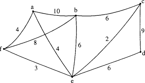
A graph G consists of a finite set of vertices V(G), which cannot be empty and a finite set of edges, E(G), which connect pairs of vertices. The number of vertices of G is called the order of G. The number of edges in G is represented by |E| and the number of vertices by |V|.
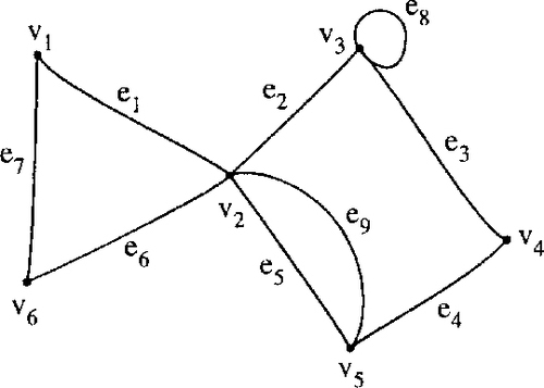
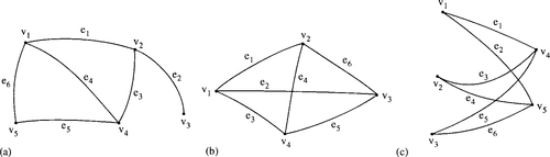
The graph in Figure 19.2 has |V| = 6 and |E| = 9.
Incidence, adjacency, and neighbours
Two vertices are adjacent if they are joined by an edge. In Figure 19.2, v3 is adjacent to v4 and is also said to be a neighbour of v4. The edge which joins the vertices is said to be incident to them. That is e3 is incident to v3 and v4.
Multiple edges and loops, simple graphs
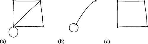
Two or more edges joining the same pair of vertices are multiple edges. An edge joining a vertex to itself is called a loop. In Figure 19.2 edges e5 and e9 are multiple edges and e8 is a loop. A graph containing no multiple edges or loops is called a simple graph. There is an example of a simple graph in Figure 19.3.

Isomorphism
Graphs are isomorphic to each other if one can be obtained from a redrawing of the other one. Some isomorphic graphs are shown in Figure 19.4.

Weighted graph
A weighted graph has a number assigned to each of its edges, called its weight. The weight can be used to represent distances or capacities. A weighted graph is shown in Figure 19.5.

Digraphs
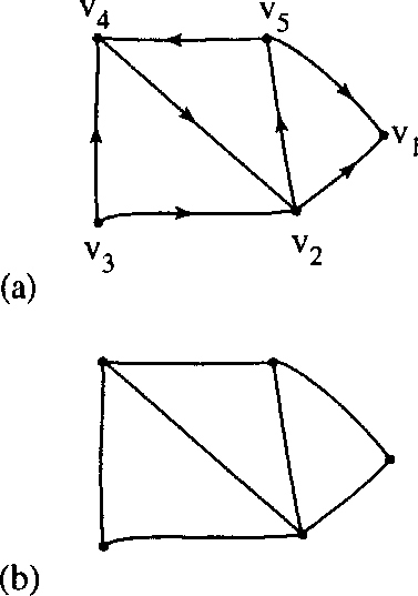
A digraph is a directed graph, that is, instead of edges in the definition of graphs we have arcs join pairs of vertices in a specified order. A digraph is shown in Figure 19.6(a).
Underlying graph
The underlying graph of a digraph D is the graph obtained by replacing each arc by an (undirected) edge as in Figure 19.6(b).
Degrees
The number of times edges are incident to a vertex, v, is called its degree, denoted by d(v). In Figure 19.2 vertex v5 has degree 3 and vertex v3 has degree 4.
A vertex of a digraph has an in-degree d–(v) and an out-degree, d+(v). In Figure 19.6(a) v5 has in-degree of 1 and out-degree of 2. Vertex v1 has in-degree 1 and out-degree 1.
The sum of the values of the degree, d(v), over all the vertices of a graph totals to twice the number of edges:
![]()
where |E| is the number of edges.
Checking this result for Figure 19.2, we find that the degrees are ![]() Summing these gives 18, which is the same as twice the number of edges.
Summing these gives 18, which is the same as twice the number of edges.
For a digraph we get
![]()
where |A| is the number of arcs.
Subgraph
A subgraph of G is a graph, H, whose vertex set is a subset of G's vertex set, and similarly its edge set is a subset of the edge set of G.
![]()
If it spans all of the vertices of G, that is, V (H) == V (G) then H is called a spanning subgraph of G. A graph G, a subgraph, and a spanning subgraph are shown in Figure 19.7.
Complete graph
A simple graph in which every pair of two vertices is adjacent is called a complete graph. Knis the complete graph with n vertices. Knhas ![]() edges. Some examples of complete graphs are shown in Figure 19.8.
edges. Some examples of complete graphs are shown in Figure 19.8.

Bipartite graph
This is a graph whose vertex set can be partitioned into two sets in such a way that each edge joins a vertex of the first set to a vertex of the second set. Some examples are given in Figure 19.9.

A complete bipartite graph is a bipartite simple graph in which every vertex in the first set is adjacent to every vertex in the second set. Km,n is the complete bipartite graph with m vertices in the first set and n vertices in the second set. Some examples of complete bipartite graphs are given in Figure 19.9(b) and (c).
Walks, paths, and circuits
A sequence of edges of the form
![]()
is a walk of from vs to vt. If these edges are all distinct then the walk is called a trail and if the vertices are also distinct then the walk is called a path. A walk or trail is closed if vs = vt. A closed walk in which all the vertices are distinct except vs and vt is called a cycle or circuit. Examples are given in Figure 19.10.

Connected graph
A graph G is connected if there is a path from any one of its vertices to any other vertex. A disconnected graph is said to be made up of components. All the graphs we have drawn so far have been connected. In Figure 19.11(a) there is a disconnected graph with two components and in Figure 19.11(b) a disconnected graph with three components.

Planar graphs
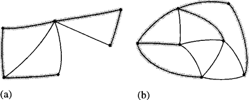
A planar graph is one which can be drawn in the plane without any edges intersecting except at vertices to which they are both incident. There is an example of a planar graph in Figure 19.12(a) and a non-planar graph in Figure 19.12(b).

19.3 Matrix representation of a graph
The incidence matrix and adjacency matrix
The incidence matrix of a graph G is a |V| ×|E| matrix. The element aij= the number of times that vertex viis incident with the edge ej.
The adjacency matrix of G is the |V| × |V| matrix. aij= the number of edges joining viand vjThe incidence matrix for the graph in Figure 19.2 is given by
and the adjacency matrix by

19.4 Trees
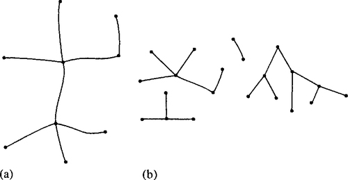
A tree is a connected graph with no cycles. A forest is a graph with no cycles but may or may not be connected (i.e. a forest is a graph whose components are trees). Figure 19.13(a) shows a tree, while Figure 19.12(b) shows a forest.
If T is a tree with at least two vertices, then it has the three properties (T1) (T2), and (T3):
(T1) There is exactly one path from any vertex viin T to any other vertex vj.
(T2) The graph obtained from T by removing any edge has two components, each of which is a tree.
![]()
Trees have many applications, particularly rooted trees. Decision trees are used to represent the possible decisions at each stage of a problem or algorithm. Probability trees can be used to analyse conditional probabilities, which we shall see in Chapter 21. Another application is to parsing of a sentence. The tree in Figure 19.14 represents the sentence ‘Fortune favours the brave'. The vertices, other than the terminal vertices, represent grammatical categories and the terminal vertices represent the words of the sentence. The same sort of idea can be used to analyse allowed constructs of statements in programming languages and the syntax of arithmetic expressions. We look at this application of trees in the next chapter on language theory.

Spanning trees
A spanning tree of a graph G is a tree T which is a spanning subgraph of G. That is, T has the same vertex set as G. Examples of graphs with spanning trees marked are given in Figure 19.15.
How to grow a spanning tree
Take any vertex v of G as an initial partial tree. Add edges one by one so each new edge joins a new vertex to the partial tree. If there are n vertices in the graph G then the spanning tree will have n vertices and n – 1 edges.
Minimum spanning tree
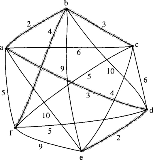
Supposing we have a group of offices which need to be connected by a network of communication lines. The offices may communicate with each other directly or through another office. In order to decide on which offices to build links between we firstly work out the cost of all possible connections. This will then give us a weighted complete graph as shown in Figure 19.16.

The minimum spanning tree is then the spanning tree that represents the minimum cost.
The greedy algorithm for the minimum spanning tree
1 Choose any start vertex to form the initial partial tree (vi).
2 Add the cheapest edge, ei, to a new vertex to form a new partial tree.
3 Repeat Step 2 until all vertices have been included in the tree.
Example 19.1
Find the minimum spanning tree for the graph representing communication links between offices as shown in Figure 19.16.
Solution We start with any vertex and choose the one marked a. Add the edge ab which is the cheapest edge of those incident to a.
Add a new edge in order to form a partial tree and choose bc, which is one of the cheapest remaining edges incident either with a or b. Now we add edge ad which is the cheapest remaining edge of those incident with a or b or c. Continuing in this manner we find the minimum spanning tree, as shown in Figure 19.17. The total cost of the communication links in our solution is found to be 2 + 3 + 3 + 2 + 4 = 14.
19.5 The shortest path problem
The weights on a graph may represent delays on a communication network or travel times along roads. A practical problem that we may wish to solve is to find the shortest path from any two vertices. The algorithm for solving this problem is illustrated in Example 19.2.
Example 19.2
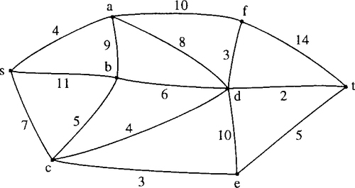
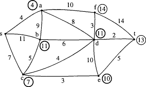
The weighted graph in Figure 19.18 represents a communication network with weights indicating the delays associated with each edge. Find the minimum delay path from s to t.
Solution
Stage 1
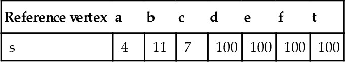
To find the path we begin at the start vertex s. s is the reference vertex for stage 1. Label all the adjacent vertices with the lengths of the paths using only one edge. Mark all the other vertices with a very high number (bigger than the sum of all the weights in the graph) in this case we choose 100. This is shown in Figure 19.19.

At the same time start to fill in a table as in Table 19.1.
Stage 2
Choose the vertex with the smallest label, that has not already been a reference vertex, so that this becomes the new reference vertex. In this case we choose vertex a. Once a vertex has been used as a reference vertex it gains a permanent label and for this reason we circle the label in bold, as in Figure 19.20 and circle the label in the table as in Table 19.2. This label represents the length of the shortest path from s to the new reference vertex. Consider any vertex adjacent to the new reference vertex and calculate the length of the path via a to this vertex. If this is less than the current temporary label on the vertex then change the label on the vertex. For instance, b is adjacent to vertex a. The length of the path to b via a is 4 + 9 = 13. This is not less than the current label of 11, so we keep the current label. However, looking at vertex d, which is adjacent to a, the length of the path via a is 4 + 8 = 12, which is shorter than the current label of d, hence we change the current label. Considering also the vertices b and f, we end up at the end of Stage 2, with the labels as given in Figure 19.20 and in Table 19.2.

Stage 3
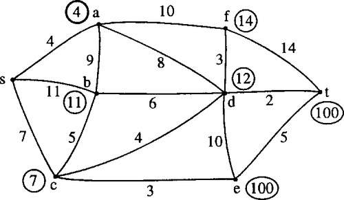
Choose the vertex with the smallest label that has not already been a reference vertex; this becomes the new reference vertex. In this case we choose vertex c, so this gains a permanent label which we circle in bold as in Figure 19.21; we also circle the label as in Table 19.3. This label represents the length of the shortest path from s to c. Consider any vertex adjacent to c which does not have a permanent label, and calculate the length of the path via c to this vertex. If this is less than the current temporary label on the vertex then change the label on the vertex. For instance, d is adjacent to vertex c. The length of the path to d via c is 7 + 4 = 11. This is less than the current label of 12 so we change the label. However, looking at vertex b, which is adjacent to c, the length of the path via c is 7 + 5 = 12 which is longer than the current label of 11, so we keep the current label. Considering also the vertex e we end up, at the end of Stage 3, with the labels as given in Figure 19.21 and Table 19.3.


Stage 4
Choose e as the new reference vertex and mark its label in bold. Compare paths via e to the labels on any adjacent vertices and re-label the vertices if the paths via e are found to be shorter. The result of this stage is shown in Figure 19.22 and Table 19.4.

Stage 5
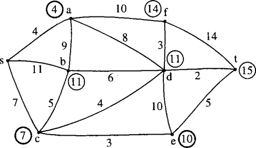
Choose b as the new reference vertex (we could choose d instead but this would make no difference to the final result) and circle its label in bold. Compare paths via b to the labels on any adjacent vertices and relabel the vertices if the paths via b are found to be shorter. The result of this stage is shown in Figure 19.23 and Table 19.5.


Stage 6
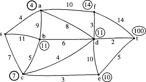
Choose d as the new reference vertex and mark its label in bold. The only vertices left without permanent labels are t and f. We find that the path via d to t gives a smaller value than the current label of 15 and hence we change the label to 11 + 2 = 13. The result of this stage is shown in Figure 19.24 and Table 19.6.


Stage 7
The remaining vertex with the smallest label is t. We therefore give t the permanent label of 13. As soon as t receives a permanent label we can stop the algorithm as this must now represent the length of the shortest path from s to t which is the result we set out to find. To find the actual path that has this length we move backwards from t looking for consistent labels. To get to t we must have gone through d as adding the label on d to the length of edge dt gives the correct value of 13. Continuing this process, we find that the shortest path is scdt and is of length 13. The final solution is shown in Figure 19.25 and Table 19.7.


19.6 Networks and maximum flow
A network is a digraph with a weight function. The weight function represents the number of links between the vertices, for example the units of traffic (channels) in a communication network, or the maximum capacity of a network of one way streets in a busy town. This weight function value is called the capacity of the arc. An example of a network is shown in Figure 19.26. s is the source and t is the sink. The capacity of an arc, ak will be referred to as c(ak). We wish to find the maximum possible flow from s the source to the sink t. That is we want to find a flow function f(ak) assigning a flow to each of the arcs which gives this maximum flow.

Flow function
A valid flow function must be such that:
2 The out-flow at any vertex equals the in-flow except at the source or the sink.
An arc is saturated if f(ak) = c(ak). The total flow is then the flow out of s (which equals the flow into t).
Finding a maximum flow
1 Assign an initial flow to each edge (this will probably be 0 flow on each arc).
2 Find a flow-augmenting path from s to t. Any arc along this flow-augmenting path may be either in the forward direction, that is, in the same direction as the path, or in the backward direction, that is, in the opposite direction to the path. If the arc along the path is in the forward direction, then it must have some ‘extra’ capacity ![]() then the extra capacity is represented by
then the extra capacity is represented by ![]() If the arc along the path is in the backward direction, then f(ak) must be greater than 0 and we assign the possible increase in flow Δk= f(ak). We can then calculate the amount that this path can augment the flow by as Δ = minimum (Δk), where we consider all the values of along the path.
If the arc along the path is in the backward direction, then f(ak) must be greater than 0 and we assign the possible increase in flow Δk= f(ak). We can then calculate the amount that this path can augment the flow by as Δ = minimum (Δk), where we consider all the values of along the path.
3 We can now change the value of the flow function along the flow-augmenting path to f(ak) + Δ (for arcs in the forward direction along the path) and f (ak) – Δ (for arcs in the backward direction along the path). We then repeat the second stage and look for another flow-augmenting path. If no more flow-augmenting paths exist, then we have found the maximum flow. This algorithm is due to Ford and Fulkerson. It can take a long while to terminate on complicated networks and better algorithms have been developed, for example, the Dinic algorithm which is not given here. We can check that we have in fact found the maximum flow in the network by finding the minimum cut. The max-flow, min-cut theorem states that the maximum value of a flow from s to t in a network is equal to the minimum capacity of a cut separating s and t.
Example 19.3
Find the maximum flow from s to t in the network shown in Figure 19.27(a). The weights on the arcs represent their capacities.

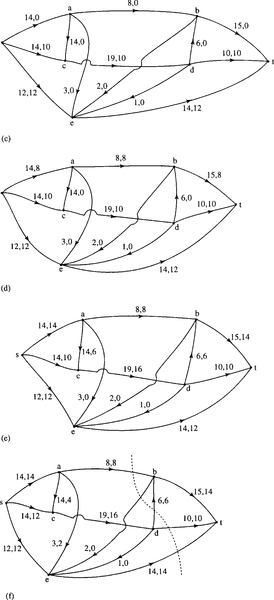
Solution We begin by identifying a flow-augmenting path s, e, t. As initially we consider the flow function to be zero then the spare capacities along the arcs are 12 and 14, the minimum of which is 12. We therefore assign a flow of 12 along the path to get Figure 19.27(b).
We spot another flow-augmenting path, s, c, d, t with a possible flow of 10 (the minimum of 14, 19, and 10). We add 10 to the flow function along this path to give Figure 19.27(c).
We identify the flow-augmenting path s, a, b, t with a possible flow of 8 (the minimum of the values of the spare capacities of 14, 8 and 15). We add 8 to the flow function along this path to give Figure 19.27(d).
Another flow-augmenting path is s, a, c, d, b, t with a possible flow of 6 (the minimum of the values of the spare capacities of 6, 14, 9, 6, 7). We add 6 to the flow function along this path to give Figure 19.27(e).
There are no more entirely forward paths but we can see one that involves an arc in the backward direction, that has a non-zero flow function. This path is s, c, a, e, t where ca is in the backward direction. We take the minimum of the spare capacity in the forward direction along with the value of the flow in the backward direction. This gives 2 as the minimum of 4, 6, 3, and 2. We add 2 to the flows on the arcs in the forward direction and subtract 2 from the flow on ca which is in the backward direction. Note that this process is equivalent to redirecting the flow. We have now reached Figure 19.27(f). We are unable to identify any more flow-augmenting paths. We can confirm that this is in fact a solution to the maximum flow problem by using the max-flow, min-cut theorem. If we look at the cut marked we see that this has a capacity of 38. To find this we add the capacities of all the arcs which cross the cut from the's end’ to the ‘t end’, that is, db, with a capacity of 6, dt with a capacity of 10 and et with a capacity of 14. This cut has a capacity of 38 in total which is the value of the flow we have found.
19.7 State transition diagrams
A state transition diagram is used to represent a finite state machine. These are used to model objects which have a finite number of possible states and whose interaction with the outside world can be described by its state changes in response to a finite number of events. A state transition diagram is a digraph whose nodes are states and whose directed arcs are transitions labelled by event names. A state is drawn as a rounded box containing an optional name. A transition is drawn as an arc with the arrow from the receiving state to the target state. The label on the arrow is the name of the event causing the transition. State transition diagrams have a number of applications. They are used in object-oriented modelling techniques to represent the life cycle of an object. They can be used as a finite state recognizer for a regular language, for instance, to describe regular expressions used as variables in computer languages.
Example 19.4
A telephone has the attributes of off-hook (TRUE, FALSE), connected (TRUE, FALSE), dialing (TRUE, FALSE), tone (dial tone, engaged, ringing, error, dead or none), and bell (ON, OFF). These can be represented as a list (off-hook, connected, dialing, tone, bell) which can take a selection of values to indicate the current state of the telephone, for example, TRUE, FALSE, FALSE, engaged, OFF indicates that the phone is off-hook, it is not connected, it is not dialing it has the engaged tone, and the bell is OFF. Use your knowledge of the operation of a telephone to give a full list of the possible states of the phone. Draw a state transition diagram to represent the life-cycle of the phone.
Solution The possible states are given in Table 19.8.
Table 19.8
The states of a telephone
| State (off-hook, connected, dialing, tone, bell) | State name |
| (TRUE, TRUE, FALSE, none, OFF) | Connected |
| (TRUE, FALSE, TRUE, none, OFF) | In process of dialing |
| (TRUE, FALSE, FALSE, dial tone, OFF) | Prepared for dialing |
| (TRUE, FALSE, FALSE, engaged, OFF) | Engaged |
| (TRUE, FLASE, FALSE, ringing, OFF) | Waiting to connect |
| (TRUE, FALSE, FALSE, error, OFF) | Incorrect number or timeout |
| (TRUE, FALSE, FALSE, dead, OFF) | Connection fault |
| (FALSE, FALSE, FALSE, none, OFF) | Idle |
| (FALSE, FALSE, FALSE, none, ON) | Incoming call |
The possible events are: Pick up receiver, replace receiver, wait, dial a number, someone calls your number. The events that are possible and the transitions that they cause depend on the current state of the phone. The state transition diagram is shown in Figure 19.28.

Example 19.5
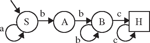
Figure 19.29 shows a deterministic finite state recognizer (DFSR) for a language consisting of strings of the letters a, b, and c. To test whether a certain string is accepted by the DFSR:
1 Start at the start state, labelled as S.
2 Take a letter from the left of the string. If possible, move along a transition arc labelled with that letter.
3 Repeat step 2 moving through the DFSR until either you find that you cannot move because there is no appropriately labelled arc or the string is exhausted. If, when the string is exhausted you have reached the halt state (marked as H in a square box) then the string has been accepted. If, when the string is exhausted you have not reached the halt state, or if at any point there are no legal moves, then the string is not accepted.
(a) show that abbc is an acceptable string,
(b) show that abbb is not an acceptable string,
(c) show that ababab is not an acceptable string.
(a) We find a path from S to H along arcs labelled abbc. To do this, we travel along arcs in the following order SS, SA, AB, BH. As this path begins with S and ends with H we have shown that the DFSR recognizes the string abbc.
(b) We look at the path labelled abbb beginning at S. The only possible path is: SSAB. As this path does not end at H we have shown that the DFSR does not recognize the string abbb.
(c) We look for a path labelled ababab. No such path exists as it would begin with the arcs SS, SA and then there is no arc out of A labelled ‘b’. As there are no more legal moves we have shown that the string is not accepted.
19.8 Summary
1 A graph consists of a set of vertices, V and a set of edges, E. A digraph is a directed graph, with arcs instead of edges. Various definitions for different types of graphs are given in Section 19.2.
2 Graphs can be represented by an incidence matrix or an adjacency matrix.
3 Various optimization algorithms have been demonstrated in this chapter, including the greedy algorithm for the minimum spanning tree and the solution to the minimum path problem. For these two examples, the weights on the graph represent lengths, costs, or delays. We have also looked at one solution to the maximum flow problem. For this problem the weights on the arcs of a digraph represent the maximum capacity of the arc and the problem is to maximise the flow through the network.
4 A state transition diagram is used to represent a finite state machine.
19.9 Exercises
19.1. From the graphs in Figure 19.30 identify any that are isomorphic.

19.2. The sequence of complete graphs K1, K2, K3, K4… can be drawn by adding a vertex to the previous member of the sequence and drawing in all the edges necessary to make the new graph complete. Using this method, show that the number of edges in the complete graph Kn can be found from the series
1 + 2 + 3 + ···+ n – 1.
19.3. For what values of n is the complete graph Kn planar?
For what values of m, n is the complete bipartite graph Km,nplanar?
19.4. (a) Find the incidence and adjacency matrices for the graphs in Figure 19.31.
(b) Show that in each case the column sum of the incidence matrix is 2 and explain this property.
(c) What are the column sums of A and what property of the graph do they represent?
19.5 Find a minimum spanning tree for the weighted graph in Figure 19.32. Is there more than one possible minimum spanning tree for this graph?
19.6 Find the shortest path from s to t in the weighted graph shown in Figure 19.33.

19.7 Find the maximum flow in the network shown in Figure 19.34. The number next to each arc is its capacity. Use the max-flow, min-cut theorem to check you have found the maximum flow.

19.8 In the network in Figure 19.35, the arcs represent communication channels which have the maximum capacity indicated. The vertices represent switching centres, which also have a maximum capacity as indicated on the vertex. By replacing each of the vertices by two vertices with a connecting arc with a capacity equal to that of the original vertex, find the maximum flow from s to t. Use the max-flow, min-cut theorem to check you have found the maximum flow.

19.9 A bank's automatic telling machine (ATM) is characterized by the following attributes {money available, card, PIN number, authorization, display, money issued }.
‘money available’ is (TRUE, FALSE) depending on whether the cash available in the machine is sufficient for the current request.
‘card’ is TRUE or FALSE.
‘PIN number’ is TRUE or FALSE indicating whether any given pin number matches for the current card
‘authorization’ is TRUE or FALSE.
‘display’ is ‘Insert card’, ‘Enter PIN’, ‘Enter amount’, ‘Take card’, ‘Take Money’, ‘Sorry – unable to complete request’.
‘money issued’ is TRUE or FALSE.
List all the possible states of the ATM and draw a state transition diagram.
19.10 Figure 19.36 shows a deterministic finite state recogniser (DFSR) for a language consisting of strings of the letters a, b, and c. Use the method of Example 19.5 to determine whether the following strings are accepted by the DFSR (a) bbbc, (b) abc, (c) acb.
