
Systems of linear equations, matrices, and determinants
13.1 Introduction
The widespread use of computers to solve engineering problems means that it is important to be able to represent problems in a form suitable for solution by a computer. Matrices are used to represent: systems of linear equations; transformations used in computer graphics or for robotic control; road, electrical and communication networks, and stresses and strains in materials. A matrix is a rectangular array of numbers of dimension m × n where m is the number of rows and n is the number of columns in the matrix. Matrices are also useful because they enable us to consider an array of numbers as a single object, represent it by a single symbol, and manipulate these symbols conveniently. In this chapter, we look at applications of matrices and arithmetic operations on matrices and some common numerical methods. We shall also look at the problem of solving systems of linear equations. The methods of solving linear systems of equations are well understood and we only need to be able to solve simple cases of such problems ‘by hand’. However, it is important to be able to express a problem in matrix form and also appreciate situations where no solution exists or where more than one solution exists. This allows to analyse the problems of ill-conditioning of systems of equations, which can lead to instability in the solution and the problem of over- or under-determinacy, where either we have too much information, leading to possibly contradictory conditions, or we have not got enough to produce a single set of solutions for the unknowns.
We shall also look at the eigenvalue problem. The technique of finding eigenvalues will become particularly important when applied to systems of differential equations which we meet in Chapter 14.
13.2 Matrices
A matrix is a rectangular array of numbers. They may also be used as a simple store of information as in the following example.
Every weekday a household orders pints of milk, loaves of bread, and yoghurt from a milk lorry. The orders for the week can be displayed as follows:

This information forms a matrix.
Transformations in a plane can be represented by using matrices, for example, a reflection about the x -axis can be represented by the matrix
(100−1)
![]()
and rotation through the angle by
(cos(θ)−sin(θ)sin(θ)cos(θ)).

We shall return to these examples later. Also in the chapter we will see that linear equations can be written in matrix form.
Notation
A matrix is represented by a capital letter A (bold) or by [aij] where aij represents a typical element in the i th row and j th column of the matrix. We represent a general matrix in the following form:
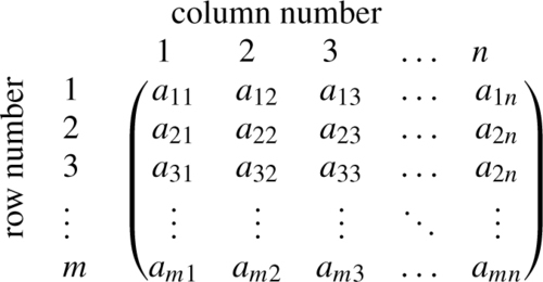
In order to refer to the element which is in the third row and the second column we can say a32. The matrix
(326182)

is a 3 × 2 matrix (read as 3 by 2) as it has 3 rows and 2 columns.
The sum and difference of matrices
The sum and difference of matrices is found by adding or subtracting corresponding elements of the matrix. Only matrices of exactly the same dimension can be added or subtracted.
Example 13.1
A=(2????1)??B=(6????2)C=(3783)D=(1221)E=(821613)F=(26312−2−6)

Find where possible: (a) A + B, (b) C + D, (c) E – F, (d) A + D.
Solution
(a) A + B = (2 1) + (6 2) = (8 3)
(b) C − D = (3783)+(1221)=(49104)![]()
(c) E + F=(821613)-(26312-2-6)=(6-4-2-639)
(d) A + D cannot be found because the two matrices are of different dimensions.
Multiplication of a matrix by a scalar
To multiply a matrix by a scalar, every element is multiplied by the scalar.
Example 13.2
If?A=(2561)
![]()
find 2A and 13![]() A
A
2A=2(2561)=(410122)13A=13(2561)=(2353213)

Multiplication of two matrices
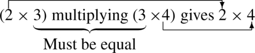
To multiply two matrices, every row is multiplied by every column. For instance, if C = AB, to find the element in the second row and the third column of the product, C, we take the second row of A and the third column of B and multiply them together, like taking the scalar product of two vectors. Multiplication is only possible if the number of columns in A is the same as the number of rows in B. For instance, if A is 2 × 3 it can only multiply matrices that are 3 × n where n could be any dimension. The result of a 2 × 3 multiplying a 3 × 4 is a 2 × 4 matrix. Notice the pattern:
Example 13.3
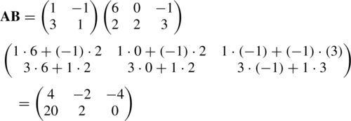
A=(1−131)B=(60−1223)

Find, if possible, AB and BA
BA cannot be found because the number of columns in B is not equal to the number of rows in A.
We can justify the practical reasons for this method of matrix multiplication as in the following two examples. In the first, we return to our household shopping example.
Example 13.4
Every weekday a household orders pints of milk, loaves of bread and yoghurt from a milk lorry. The orders for the week are as follows:

Next week, the dairy introduces a special offer and reduces its prices. The prices for this week and the next are as follows:
Calculate the cost each day for this week and the next.
Solution The cost each day is made up of the number of pints of milk times the cost of a pint plus the number of loaves of bread times the cost of a loaf plus the number of cartons of yoghurt times the cost of the yoghurt. In other words, we can find the cost each day by performing matrix multiplication
(324410224510114)(0.340.320.600.500.330.30) =(3×(0.34)+2×(0.60)+4×(0.33)3×(0.32)+2×(0.50)+4×(0.30)4×(0.34)+1×(0.60)+0×(0.33)4×(0.32)+1×(0.50)+0×(0.30)2×(0.34)+2×(0.60)+4×(0.33)2×(0.32)+2×(0.50)+4×(0.30)5×(0.34)+1×(0.60)+0×(0.33)5×(0.32)+1×(0.50)+0×(0.30)1×(0.34)+1×(0.60)+4×(0.33)1×(0.32)+1×(0.50)+4×(0.30))=(3.543.161.961.783.202.842.302.102.262.02)

The rows now represent the days of the week and the columns represent this week and the next week. Hence, for instance, the cost for Thursday of next week is given by the element a42=2.10.
Example 13.5
Figure 13.1 represents a communication network where the vertices a,b,f,g represent offices and vertices c,d,e represent switching centres. The numbers marked along the edges represent the number of connections between any two vertices. Calculate the number of routes from a,b to f,g.

Solution The number of routes from a to f can be calculated by taking the number via c plus the number via d plus the number via e. In each case, this is given by multiplying the number of connections along the edges connecting a to c, c to f, etc giving the number of routes from a to f as: 3 × 2 + 4 × 6 + 1 × 1.
We can see that we can get the number of routes by matrix multiplication. The network from ab to cde is represented by:

and from cde to fg by

So, the total number of routes is given by
(341213)(216312)??=(3×2+4×6+1×13×1+4×3+1×22×2+1×6+3×12×1+3×1+3×2)

Hence, by interpreting the rows and columns of the resulting matrix we can see that there are 31 routes from a to f, 17 from a to g, 13 from b to f and 11 from b to g.
The unit matrix
The unit matrix is a square matrix which leaves any matrix, A, unchanged under multiplication. If A is a square matrix, then
AI=IA=A
The unit matrix has 1s on its leading diagonal and 0s elsewhere. In two dimensions
I=(1001)

In three dimensions
I=(100010001).

Example 13.6
A=(2−101),?B=(32)

Show that AI =IA =A and IB =B.

The transpose of a matrix
The transpose of a matrix is obtained by interchanging the rows and the columns. The transpose of a matrix A is represented by AT.
Example 13.7
Given
A=(2−163),?B=(218−101)
![]()
find ATand BT
Solution The first row of A is (2–1) therefore this is the first column of AT. The second row of A is (6 3) therefore this is the second column of AT. This gives ATas follows.
AT=(26−13)

Similarly
BT=(2−11081)
Some special types of matrices
A square matrix has the same number of rows as columns.
(2−163)

is a square matrix of dimension 2.
(862−310321)
is a square matrix of dimension 3.
A square matrix has a leading diagonal, which comprises the elements lying along the diagonal from the top left-hand corner to the bottom righthand corner as marked below. These elements have the same row number as they have column number.

The leading diagonal is shown by the dotted line in the above matrix.
A diagonal matrix is a square matrix which has zero elements everywhere except, possibly, on its leading diagonal, for example
(4000−20003)

An upper triangular matrix is a square matrix which has zeros below the leading diagonal, for example
(112066008)

A lower triangular matrix has zeros above the leading diagonal, for example
(1003−10682)

A symmetric matrix is such that A T =A, that is, the elements are symmetric about the leading diagonal, for example
A=(16−360−2−3−28),?B=(1661)
are symmetric matrices. If you take the transpose of one of these matrices they result in the original matrix.
A skew-symmetric matrix is such that AT = −A.
Example 13.8
Show that
A=(06−60)
![]()
is skew symmetric.
Solution
AT=(0−660)
![]()
Multiplying A by −1, we get
−A=(0−660)

We can see that AT = −A and hence we have shown that A is skew symmetric.
Hermitian matrix
A Hermitian matrix is such that A*T =A.
Example 13.9
Show that
A=(37+j27−j2−2)?and?B=(23e−j23ej21)

are Hermitian.
Solution Taking the complex conjugates of each of the elements in A and B gives
A*=(37−j27+j2−2)?and?B*=(23ej23e−j21)

Now taking the transposes of A and B, we get
A*T=(37+j27−j2−2)?and?B*T=(23e−j23ej21)

So we can see that
A*T=A?and?B*T=B
![]()
showing that they are Hermitian.
In the rest of this chapter we shall assume that our matrices are real. A column vector is a matrix with only one column, for example
v=(123)

A row vector is a matrix with only one row, for example
v=(1?2?3).
![]()
The inverse of a matrix
The inverse of a matrix A is a matrix A−1 such that AA −1 = A−1 A =I (the unit matrix).
Example 13.10
Show that
(131313−23)

is the inverse of
(211−1).

Solution Multiply:

Also

Not all matrices have inverses and only square matrices can possibly have inverses. A matrix does not have an inverse if its determinant is 0.
The determinant of
(abcd)
![]()
is given by
|abcd|=ad−cb

If the determinant of a matrix is 0 then it has no inverse and the matrix is said to be singular. If the determinant is non- zero then the inverse exists. The inverse of the 2 × 2 matrix
(abcd)

is
1(ad−cb)(d−b−ca)

That is, to find the inverse of a 2 × 2 matrix, we swap the diagonal elements, negate the off-diagonal elements, and divide the resulting matrix by the determinant.
Example 13.11
Find the determinants of the following matrices and state if the matrix has an inverse or is singular. Find the inverse in the cases where is exists and check that AA −1 =A −1 A =I
(a)?(−1321),?(b)(6−2−31),?(c)(1√2−1√21√21√2).
Solution
(a)|−1321|=(−1)×1−2×3=−7.

As the determinant is not zero the matrix
(−1321)

has an inverse found by swapping the diagonal elements and negating the off-diagonal elements, then dividing by the determinant. This gives
1−7(1−3−2−1)=17(−1321).

Check that AA −1 =I
(−1321)17(−1321)=17((−1)(−1)+(3)(2)(−1)3+(3)(1)(2)(−1)+(1)(2)(2)(3)+(1)(1))=(1001)

and that A −1 A =I
17(−1321)(−1321)?=17((−1)(−1)+(3)(2)(−1)3+(3)(1)(2)(−1)+(1)(2)(2)(3)+(1)(1))=(1001).(b)|6−2−31|=6⋅1−(−3)(−2)=0

As the determinant is zero the matrix
(6−2−31)

has no inverse. It is singular.
(c)?|1√2−1√21√21√2|=1√21√2−(−1√2)1√2=1.

Therefore, the matrix is invertible. Its inverse is given by swapping the diagonal elements, and negating the off-diagonal elements, and then dividing by the determinant. This gives
(1√21√2−1√21√2)

Check that AA −1 =I:
AA−1=(1√2−1√21√21√2)(1√21√2−1√21√2)=(1001)

Similarly, A−1 A =I.
Solving matrix equations
To solve matrix equations, we use the same ideas about equivalent equations that we have used before. As in ordinary equations, we can ‘do the same things to both sides’ in order to find equivalent equations. It is important to remember that division by a matrix has not been defined. In order to ‘undo’ matrix multiplication we have to multiply by an inverse matrix, where it exists, and we need to specify whether we are pre- or post-multiplying. This is necessary because matrices do not obey the commutative law (AB ≠ BA). If we pre- or post-multiply both sides of an equation by a matrix we must also be able to justify that the dimensions of the expressions are such that the multiplication is possible. Also if we add or subtract a matrix from both sides of the equation it must have exactly the same dimension as the current matrix expression.
Example 13.12
Given that A, B, and C are matrices and AB =C where A and B are non-singular, find expressions for B and A.
Solution In this case, we are told that A and B are invertible, so they must be square and therefore C must also be square and of the same dimension. To find B we wish to ‘get rid’ of the A term on the left-hand side. We pre-multiply both sides of the equation by A−1
AB =C and given A is invertible
⇔ A−1AB=A−1C.
Now using A−1 A = I, the unit matrix, we have
IB = A−lC.
As the unit matrix multiplied by any matrix leaves it unchanged, we have
⇔ B=A−1C.
To find an expression for A, use
AB =C
given that B is invertible, we post-multiply by B−1
⇔ABB−1 = CB−1.
Now using BB−1=I, the unit matrix, we have
AI =CB−1.
As the unit matrix multiplied by any matrix leaves it unchanged, we have
⇔A =CB−1.
Remember that it is always important to specify whether you are pre- or post-multiplying when solving matrix equations. A term like B−1 AB cannot be simplified because we cannot swap the order, as we would do with numbers.
13.3 Transformations
On a computer graphics screen an object is represented by a set of coordinates, either with reference to the screen origin or with reference to the origin of some window created by the graphical user interface (GUI). We may wish to move the object around inside its window. We shall consider in this section only two-dimensional objects as dealing with three-dimensional objects would add the complication of needing to represent a perspective view. Ideas about transformations are also important when considering movement of a robotic arm.
There are three ways of moving an object without affecting its overall size or shape: rotation, reflection and translation. We could also stretch it or compress it in some direction – the operation of scaling.
We shall look at how to perform these operations using matrices and vectors. We can check that the operations performed are those that we expected by looking at the effect on some simple shapes. In most of these examples, we look at the effect of a unit square at the origin, defined by the points A (0,0), B(1,0), C (1,1), D (0,1). The outcome of the transformation is called the image which we will represent by the points A′, B′, C′, D′. The transformation, T, is a function whose domain and codomain is the plane (which is referred to as ℝ2![]() ). The term ‘mapping’ is also used in this context. It has exactly the same meaning as function, but is more often used when referring to geometrical problems.
). The term ‘mapping’ is also used in this context. It has exactly the same meaning as function, but is more often used when referring to geometrical problems.
Rotation
To perform a rotation through an angle θ, we multiply the position vector of the point
(xy)
![]()
by a matrix of the form
(cos(θ)−sin(θ)sin(θ)cos(θ)).

Example 13.13
Find and draw the image of the unit square with vertices A(0,0), B(1,0), C(1,1), D(0, 1) after rotation through 30° about the origin.
Solution Rotation through 30° about the origin is found by multiplying the position vectors of the points by
(cos(30∘)−sin(30∘)sin(30∘)cos(30∘))≈(0.866−0.50.50.866)

To find the image of the unit square, we multiply the position vectors of the vertices by this matrix
(0.866−0.50.50.866)(00)=(00) (0.866−0.50.50.866)(10)=(0.8660.5)(0.866−0.50.50.866)(11)=(0.3661.366)(0.866−0.50.50.866)(01)=(−0.50.866)
This transformation is shown in Figure 13.2.

Sometimes, it is useful to be able to rotate the axes rather than the object. For instance, the object may be held by a robotic arm and we want the arm to rotate but keep the orientation of the object the same. This is picture for the tea drinking robot in Figure 13.3.

In this case, if we rotate the axes Ox, Oy, by the position of the object remains the same but even so has new coordinates relative to the the transformed axes OX, OY. If the axes rotate through 30°, then the object moves relative to the axes by – 30°. So to rotate the axes by we multiply the position vectors of the points
(xy)
![]()
by the matrix
(cos(−θ)−sin(−θ)sin(−θ)cos(−θ))=(cos(θ)sin(θ)−sin(θ)cos(θ)).
Example 13.14
A unit square has vertices A(0,0), B(1,0), C (1,1), D(0, 1) relative to axes Ox, Oy. The axes are rotated through 30° to OX, OY, without moving the square. Find the coordinates of the vertices relative to the new axes OX, OY.
Solution The effect of rotating the axes through 30° is found by multiplying the position vectors of the points by
(cos(30∘)sin(30∘)sin(−30∘)cos(30∘))=(0.8660.5−0.50.866).
To find the coordinates of the unit square relative to the new axes, we multiply the position vectors of the vertices by this matrix
(0.8660.5−0.50.866)(00)=(00) (0.8660.5−0.50.866)(10)=(0.866−0.5)(0.8660.5−0.50.866)(11)=(1.3660.366)(0.8660.5−0.50.866)(01)=(0.50.866).
This is shown in Figure 13.4.

Reflection
To perform a reflection in the x-axis, we multiply the position vectors of the points
(xy)
![]()
by the matrix
(100−1)

This has the effect of keeping the x -coordinate the same whilst changing the sign of the y-coordinate, hence turning the object upside down.
To perform a reflection in the y-axis, we multiply the position vectors of the points
(xy)
![]()
by the matrix
(−1001)

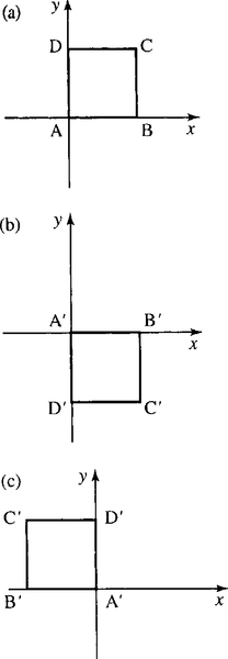
which keeps the y-value constant while changing the sign of the x-coordinate. The effect on the unit square is shown in Figure 13.5.
Translation
Translation in the plane cannot be represented by multiplying by a 2 × 2 matrix. To perform a translation, we add the vector representing the translation to the original position vectors of the points.
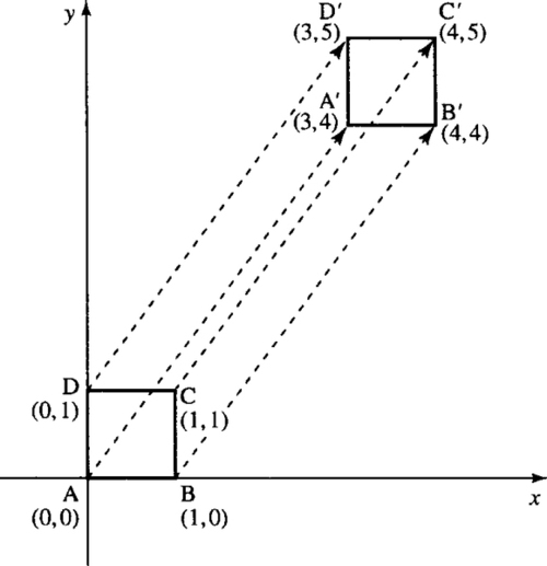
Example 13.15
Find and draw the image of the unit square with vertices A(0,0), B(1,0), C(1,1), D(0,l) after translation through
(34).
![]()
Solution Add
(34)
![]()
to the position vectors of the vertices, that is
v+(34)

which gives A′ as (3,4), B′ as (4,4), C′ as (4,5), and D′ as (3,5). This transformation is shown in Figure 13.6.
It is again often useful to consider what happens if the object stays where it is and the axes are translated. If the axes are translated through
(34)
![]()
then the object appears to move relative to the axes by
(−3−4).

Therefore, we subtract
(34)
![]()
from the coordinates defining it. This is shown in Figure 13.7.

Scaling
To scale in the x-direction, we multiply the position vectors of the points
(xy)
![]()
by a matrix
(Sx001)

where Sxis the scale factor. Under this transformation, vectors that have no x-component will be unaffected. To scale in the y-direction, we multiply the position vectors of the points
(xy)
![]()
by a matrix
(100Sy)

where Sy is the scale factor. Under this transformation, vectors that have no y-component will be unaffected.
The effect on the unit square of scaling by 2 in the x -direction is shown in Figure 13.8(b) and of scaling by 3 in the y-direction is shown in Figure 13.8(c).

Combined transformations
Example 13.16
Find the coordinates of the vertices of the unit square after: (a) rotation about the origin through 50° followed by a translation of (–1, 2); (b) translation of (–1, 2) followed by rotation about the origin through 50°.
Solution (a) We can write this combined transformation as
p′ =Rp + t
where p′ is the position vector of the image point, p is the position vector of the original point, R is the matrix representing the rotation, and t is the vector representing the translation.
In this case
R=(cos(50∘)−sin(50∘)sin(50∘)cos(50∘))≈(0.643−0.7660.7660.643)
and
t=(−12),?p′=(x′y′),?p=(xy)

So we have
(x′y′)=(0.643−0.7660.7660.643)(xy)+(−12)

For the coordinates of A′ substitute x =0 and y =0 giving
(x′y′)=(0.643−0.7660.7660.643)(00)+(−12)=(00)+(−12)=(−12)
for B′
(x′y′)=(0.643−0.7660.7660.643)(10)+(−12)=(0.6430.766)+(−12)=(−0.3572.766)
for C′
(x′y′)=(0.643−0.7660.7660.643)(11)+(−12)=(−0.1231.409)+(−12)=(−1.1233.409)
for D′
(x′y′)=(0.643−0.7660.7660.643)(01)+(−12)=(−0.7660.643)+(−12)=(−1.7662.643)

The image of the unit square is pictured in Figure 13.9(b).
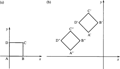
(b) We can write this combined transformation as
p″= R(p + t)
where p″ is the position vector of the image point, p is the position vector of the original point, R is the matrix representing the rotation, and t is the vector representing the translation. We have put the brackets in to
indicate that the translation is performed first. As before
R=(cos(50∘)−sin(50∘)sin(50∘)cos(50∘))≈(0.643−0.7660.7660.643)

and
t=(−12),?p″=(x″y″),?p=(xy)

So we have
(x″y″)=(0.643−0.7660.7660.643)((xy)+(−12))
which is the same as
(x″y″)=(0.643−0.7660.7660.643)(x−1y+2)
For the coordinates of A″, substitute x =0 and y =0 giving
(x″y″)=(0.643−0.7660.7660.643)(0−10+2)=(0.643−0.7660.7660.643)(−12)=(−2.1750.52)

for B″
(x″y″)=(0.643−0.7660.7660.643)(1−10+2)=(0.643−0.7660.7660.643)(02)=(−1.5321.286)

for C″
(x″y″)=(0.643−0.7660.7660.643)(1−11+2)=(0.643−0.7660.7660.643)(03)=(−2.2981.929)

for D′
(x″y″)=(0.643−0.7660.7660.643)(0−11+2)=(0.643−0.7660.7660.643)(−13)=(−2.9411.163)

The image of the unit square is pictured in Figure 13.9(b).
Note that the order of the transformations is important.
Sometimes, we might need to use a trick of temporarily moving the axes in order to perform certain transformations. Supposing we want to scale by 2 along the line x =y we can rotate the axes temporarily so that the new X -axis lies along the line that was previously x =y, then perform X scaling, and then rotate back again, so the axes are back in their original position. This is done in the next example.
Example 13.17
Find a matrix that performs scaling by a factor of 2 along the direction x =y and draw the image of the unit square defined by the vertices
A(−12,−12),B(12,−12),C(12,12),D(−12,12).

Solution First, we rotate the axes by 45°, so that the OX -axis will lie along the line that was previously x =y. This is pictured in Figure 13.10.

The matrix that transforms the coordinates so they are relative to the new axes at an angle of 45° is given by:
(cos(45∘)sin(45∘)−sin(45∘)cos(45∘))
A scaling of 2 in the X -direction is then performed by multiplying by
(2001)

We then need to rotate the axes back to their original position, that is, rotate the axes by −45°, this is done by multiplying by
(cos(−45∘)sin(−45∘)−sin(−45∘)cos(−45∘))=(cos(45∘)−sin(45∘)sin(45∘)cos(45∘))

Putting the three transformation matrices together we get
(cos(−45∘)sin(−45∘)−sin(−45∘)cos(−45∘))(2001)(cos(45∘)−sin(45∘)sin(45∘)cos(45∘))

which gives the matrix that represents a scaling along the line x = y.
Using cos (45∘)=1√2=sin(45∘), we get.
(1√2−1√21√21√2)(2001)(1√21√2−1√21√2)

Taking out the two factors of 1√2![]() gives
gives
12(1−111)(2001)(11−11)
Multiplying the second two matrices gives
12(1−111)(22−11)
and multiplying out the remaining two matrices gives
12(3113)=(32121232)

We can now multiply the position vectors representing the vertices of the square
(32121232)(−12−12)=(−1−1)(32121232)(12−12)=(12−12)(32121232)(1212)=(11)(32121232)(−1212)=(−1212)

The transformed figure is shown in Figure 13.11. We can see that has been stretched along the x = y direction but has not been scaled along the other diagonal. The image is no longer a square but a rhombus.
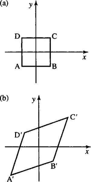
 B (12,−12),
 C (12,12)
 , D (−12,12)
 .(b) The image after scaling by 2 along the line y = x.
Example 13.18
Find a transformation that will rotate any point p about (1,1) through an angle of 90°.
Solution To rotate about a point not at the origin, we translate the origin temporarily, rotate, and then translate the origin back again.
Rotation through 90° is performed by multiplying by
(cos(90∘)−sin(90∘)sin(90∘)cos(90∘))=(0−110)

The combined transformation on a point p can be represented by
p′=(0−110)(p−(11))+(11).

13.4 Systems of equations
Example 13.19
Using Ohm's law and Kirchoff's laws for the electrical network in Figure 13.12, show that
I1−I2−I3=03I2−2I3=07I1+2I3=8


Solution Kirchoff's laws for an electrical network are as follows:
Kirchoff's voltage law (KVL): The sum of all the voltage drops around any closed loop is zero. This can also be expressed as: the voltage impressed on a closed loop is equal to the sum of the voltage drops in the rest of the loop.
Kirchoff's current law (KCL): At any point of a circuit, the sum of the in-flowing currents is equal to the sum of the out-flowing currents.
By Ohm's law we know the voltage drop across a resistor is given by V =IR, where R is the resistance of the resistor. Two loops have been identified in Figure 13.12 and by using KVL and Ohm's law in loop 1 we get
3I2−2I3=0.
![]()
Now looking at loop 2, we get
3I1−8+4I1+2I3=0?⇔?7I1+2I3=8.

Finally, we use the current law at one of the nodes to give
I1=I2+I3?⇔?I1−I2−I3=0
![]()
Finally, we can list all the equations we have found
I1−I2−I3=03I2−2I3=07I1+2I3=8

and the problem is now to find a solution which satisfies all of these equations simultaneously.
This is called a system of equations. In many electrical networks, there will be far more than three unknown currents. In such situations, it is impractical to solve the equations without the use of a computer. However, we can discover a number of important principles and problems involved in solving systems of linear equations by looking at some simple cases. The first problem we have is that it is possible to get more that these three equations from the network given in Figure 13.12. Using KVL in the outer loop would give
7I1+3I2=8
![]()
and KCL at the other node gives
I2+I3=I1?⇔?−I1+I2+I3=0
![]()
We therefore have five equations and only three unknowns.
Luckily, it is possible to show that these equations are a consistent set, that is, it is possible to find a solution. We shall return to solve for I1,I2, and I3 later. First, we shall examine all the possibilities when we have only two unknown quantities.
Systems of equations in two unknowns
The equation
ax+by=c
![]()
where a, b, c are constants is a linear equation in two unknowns (or variabies) x and y. Because there are two unknowns we need two axes to represent it, and therefore the graph can be drawn in a plane.
Because the graph only involves terms in x, y and the constant term and no other powers of either x or y, we know that the graph of the equation is a straight line, as we saw in Chapter 2. Examples of graphs of linear equations in two unknowns are given in Figure 13.13.

We call a solution to the equation a pair of values for x and y which satisfy the equation; that is, when they are substituted they give a true expression. A solution to the equation x + y = 1 is x =0.5, y =0.5 because if we substitute these values we obtain a true expression:
0.5+0.5=1.
![]()
However, there are many other solutions to x + y =1, for instance x =2, y =−1 or x =2.5, y =−1.5, etc. We say that the equation is indeterminate because there are any number of solutions to the equation x + y=1. In fact, any point on the line x + y = 1 is a solution to the equation. We can express the solutions in terms of x or y (e.g. x = 1 − y) therefore the solutions are (1 − y, y) where y can be any number. Alternatively y = 1 − x gives solutions (x, 1 − x) where x can be any number.
A system of two linear equations with two unknowns
We want to find values for x and y which solve both a1x + b1y = cl and a2x + b2y =c2 simultaneously. The problem could be expressed as
(a1x+b1y=c1)∧(a2x+b2y=c2)
![]()
When we talk of systems of equations it is understood that we want all of the equations to hold simultaneously so they are usually just listed as
a1x+b1y=c1a2x+b2y=c2

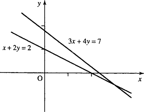
Each equation can be represented geometrically by a straight line. For example, the system
3x+4y=7x+2y=2

can be represented by the pair of straight lines as in Figure 13.14.
We can find the point where the two straight lines cross by using substitution as follows.
Example 13.20
Solve the following system of equations using substitution:
3x+4y=7x+2y=2.

Solution We begin by numbering the equations in order to identify them
3x+4y=7
x+2y=2
From Equation (13.2) we can express x in terms of y as
x + 2y =2 ⇔ x =2 − 2y (subtracting 2y from both sides)
Now substitute x =2 − 2y into Equation (13.1) to give
3(2−2y)+4y=7?⇔?6−6y+4y=7?⇔?6−2y=7?⇔?−2y=1?(subtracting?6?from?both?sides)?⇔?y=−12?(dividing?both?sides?by−2)?⇔?y=−0.5

Now we can use x =2 − 2y to find x by substituting y=−0.5 to give
x=2−2(−0.5)?⇔?x=2+1?⇔?x=3

The solution is given by x =3 and y =−0.5, which can be represented by the pair of values for (x, y) of (3, 0.5).
An alternative method of solution is to use elimination.
Example 13.21
Solve the following system of equations using elimination:
3x+4y=7x+2y=2.
Solution To solve the system of equations we look for a way of adding or subtracting multiples of one equation from the other in order to eliminate one of the variables. Multiply the second equation by 3 and leave the first the same. We choose these numbers in order to get the coefficients of x in both equations to be the same.
3x+4y=73x+6y=6.
Subtract the equations to give
−2y=1⇔y=−12=−0.5.
![]()
Substitute this into the first equation to give
3x+4(−0.5)=7?⇔?3x−2=7?⇔?3x=9?⇔?x=3.

The solution is given by x =3 and y =−0.5, which can be represented by the pair of values for (x, y) of (3, −0.5).
The point (3, −0.5) is the point on the graph where the two lines cross. This is the only point which lies both on the first graph and the second graph. It is the only point which satisfies both equations simultaneously. Hence, we say there is a unique solution to the system of equations. The system of equations is said to be determined because there is a single solution. The system of equations is also said to be consistent because it is possible to find a solution.
We could have the system of equations:
x+2y=12x+4y=2.

If we plot these lines we find that they are coincident, that is, one line lies on top of the other as in Figure 13.15.

In this case, the second equation, 2x + 4y =2, can be obtained by multiplying the first equation by 2. We say that the equations are dependent. Two equations are dependent if one can be obtained from the other by multiplying by a constant or by adding a constant to both sides. As any point that lies on x + 2 y =1 also lies on 2x + 4 y =2, there is no unique solution to the system of equations.
We say that the system of equations is indeterminate as there exist any number of solutions to the system, that is, the system reduces to only one equation. However, the system of equations is said to be consistent, because at least one solution exists.
Example solutions are:
x=2,?y=0.5?or?(2,−0.5)x=3,?y=−1?or?(3,−1)x=4,y=−1.5?or?(4,−1.5)
The solution set can be written as (x, (1 − x) /2), where x can take any value or as (1 − 2y, y), where y can take any value.
If we try to use elimination to solve the equations
x+2y=12x+4y=2

we find that one equation reduces to 0 =0, that is, a condition that is always true.
Example 13.22
Solve, using elimination:
x+2y=12x+4y=2.

Solution
x+2y=12x+4y=2

multiply the first equation by 2 to give
2x+4y=22x+4y=2

On subtraction we get
0=0
![]()
which is always true, thus indicating that the system of equations is indeterminate. The solutions are therefore any points lying on the line x + 2y =1.
The third possibility for a system of equations is one that has no solutions at all. Such a system is as follows:
x+2y=12x+4y=5

If we plot these equations we find that they are parallel, as in Figure 13.16.

From the geometrical interpretation, it is therefore clear that no solution exists to this system of equations as no point on the line x + 2 y =1 lies on the line 2x + 4 y =5. We say that the system of equations is inconsistent because no solutions exist.
If we used elimination to attempt to solve an inconsistent system of equations like these, then we will find that we will get an impossible condition, such as
0=3
![]()
which is false. This situation indicates that there are no solutions and the equations are inconsistent.
Example 13.23
Solve, using elimination
x+2y=12x+4y=5.
Solution Multiply the first equation by 2 to give
2x+4y=22x+4y=5.

Subtracting the equations, we get
0=−3.
![]()
This condition is false. This indicates that the system of equations are inconsistent and there are no solutions.
We can express systems of equations in matrix form as
Av =b
where A is the matrix of coefficients,
v=(xy)

and b is the vector of constants on the right-hand side of the equations. For the three cases we have looked at in Examples 13.21–13.23, we get the following:
Case 1:
3x+4y=7x+2y=2

which can be represented in matrix form as
(3412)(xy)=(72).

Case 2:
x+2y=12x+4y=2
which can be represented in matrix form as
(1224)(xy)=(12).

Case 3:
x+2y=12x+4y=5

which can be represented in matrix form as
(1224)(xy)=(15).
We can look at the determinants of the coefficient matrices in order to help us analyse the system.
For Case 1 (the system with a unique solution) we find
|3412|=(3⋅2)−(1⋅4)=6−4=2.

The fact that the determinant of the matrix of coefficients is non-zero shows that the system of equations has a unique solution.
For Case 2 (the system with many solutions) we find
|1224|=(1⋅4)−(2⋅2)=0.

If we replace any column in this determinant by the constant terms
(12)
![]()
we get the determinants
|1122|=(1⋅2)−(2⋅1)=0

and
|1224|=0.

This can be shown to hold in general. If all the determinants formed in this way are 0 then we have indeterminacy in the solutions. That is, there will be many solutions to the system.
For Case 3 (the system with no solutions) we find
|1224|=(1⋅4)−(2⋅2)=0

If we replace any column in this determinant by the constant terms
(15)
![]()
we get the determinants
|1125|=(1⋅5)−(2⋅1)=3

and
|1254|=(1⋅4)−(2⋅5)=−6
This can be shown to hold in general. If the determinant of the matrix of coefficients is zero but anyone of the determinants formed using the vector of constant terms are non-zero, then this shows that the system is inconsistent and there are no solutions.
We can summarize the results of this section as follows. For a system of equations (assuming we have as many equations as unknowns) there are three possibilities
Case 1: A determined system has a unique solution which can be found by using elimination. Geometrically, the solution is a single point which (in the case a a system in two unknowns) represents the intersection of the two lines. The determinant of the coefficients is non-zero. The system is both consistent and determined.
Case 2: An undetermined system has many solutions. If elimination is used to solve the system it will result in a condition like 0 =0, which is always true. Geometrically the solutions lie (for a system in two unknowns) anywhere along a line. The determinant of the coefficients is zero, as are any determinants found by replacing a column in the matrix of coefficients by the vector of constant terms. The system is undetermined but consistent (as there are solutions).
Case 3: An inconsistent system has no solutions. If elimination is used to solve the system it will result in a condition like 0 =3, which is always false. Geometrically, for a system in two unknowns, the system is represented by parallel lines which have no points in common, hence no solutions. The determinant of the coefficients is zero but at least one of the determinants found by replacing a column in the matrix of coefficients by the vector of constant terms is non-zero. The system is inconsistent.
For Case 1, the solution of the system can be found by using the inverse of the matrix of coefficients. We can represent the system by
Av =b.
As the determinant of A is non-zero, we know that A has an inverse A−1. We pre-multiply both sides of the matrix equation by A−1 giving A−lAv =A−lb
as A−1 A =I, the unit matrix and Iv =v
we get
v =A−lb
Av =b ∧ |A| ≠ 0 ⇔ v ⇔ A−lb.
Example 13.24
Solve
3x+4y=7x+2y=2
by finding the inverse of the matrix of coefficients.
Solution The system can be expressed as
(3412)(xy)=(72).

As we know that if Av =b and A is invertible then
v=A−1b
![]()
and in this case we have
A=(3412)?and?b=(72).
Then to find the solution we find the inverse of
(3412).

We know that the inverse of
(abcd)

is
1(ad−cb)(d−b−ca)

this gives the inverse of
(3412)

as
1(3⋅2)−(4⋅1)(2−4−13)=12(2−4−13)

Using x =A−1 b gives
(xy)=12(2−4−13)(72)=12(6−1)=(3−0.5)

So the solution of this system of equations is x =3 and y = −0.5.
For a 2 × 2 system, this method of solving a system of equations is quite straightforward. However, for larger systems a solution by finding the inverse involves nearly twice as many operations as that by elimination of variables and therefore should not be used as a method of solving equations.
Equations with three unknowns
For three unknowns we need three axes to represent the equations. Each equation is represented by a plane, for example, Figure 13.17 shows the plane which represents the equation x + y + z =1.

Two planes, if they intersect, will intersect along a line and if a third independent equation is given then the three planes will intersect at a point. More than three unknowns cannot be represented geometrically.
However many unknowns there are in a system of equations, the three types of systems which we identified as Cases 1–3 remain as do the methods to be used to distinguish between a determined, indeterminate, and inconsistent system.
We shall later look at finding the determinant and inverse of larger matrices, but first we look at a systematic way of doing elimination which is suitable for a computer solution of a system of equations.