
Sets and functions
1.1 Introduction
Finding relationships between quantities is of central importance in engineering. For instance, we know that given a simple circuit with a 1000 Ω resistance then the relationship between current and voltage is given by Ohm's law, I =V /1000. For any value of the voltage V we can give an associated value of I. This relationship means that I is a function of V. From this simple idea there are many other questions that need clarifying, some of which are:
1. Are all values of V permitted? For instance, a very high value of the voltage could change the nature of the material in the resistor and the expression would no longer hold.
2. Supposing the voltage V is the equivalent voltage found from considering a larger network. Then V is itself a function of other voltage values in the network (see Figure 1.1). How can we combine the functions to get the relationship between this current we are interested in and the actual voltages in the network?

3. Supposing we know the voltage in the circuit and would like to know the associated current. Given the function that defines how current depends on the voltage can we find a function that defines how the voltage depends on the current? In the case where I =V /1000, it is clear that V =1000I. This is called the inverse function.
Another reason exists for better understanding of the nature of functions. In Chapters 5 and 6, we shall study differentiation and integration. This looks at the way that functions change. A good understanding of functions and how to combine them will help considerably in those chapters.
The values that are permitted as inputs to a function are grouped together. A collection of objects is called a set. The idea of a set is very simple, but studying sets can help not only in understanding functions but also help to understand the properties of logic circuits, as discussed in Chapter 10.
1.2 Sets
A set is a collection of objects, called elements, in which the order is not important and an object cannot appear twice in the same set.
Example 1.1
Explicit definitions of sets, that is, where each element is listed, are:
A?=?{a,?b,?c}B?=?{3,4,6,7,8,9}C?=?{Linda,?Raka,?sure,?Joe,?Nigel,?Mary}

a ∈ A means ‘a is an element of A’ or ‘a belongs to A,; therefore in the above examples:
3 ∈ B
Linda ∈ C
The universal set is the set of all objects we are interested in and will depend on the problem under consideration. It is represented by ε.
The empty set (or null set) is the set with no elements. It is represented by ϕ or {}.
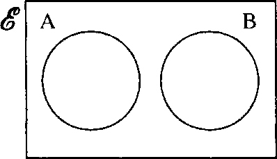
Sets can be represented diagrammatically – generally as circular shapes. The universal set is represented as a rectangle. These are called Venn diagrams.
Example 1.2
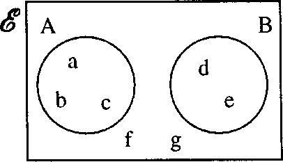
ɛ?=?{a,?b,?c,d,?e,?f,?g},?????????????A?=?{a,?b,?c},??????????B={d,?e}
![]()
This can be shown as in Figure 1.2.
We shall mainly be concerned with sets of numbers as these are more often used as inputs to functions.
Some important sets of numbers are (where ‘ … ’ means continue in the same manner):
The set of natural numbers ![]() = {1,2,3,4,5, … }
= {1,2,3,4,5, … }
The set of integers ![]() = { … −3, −2, −1,0, 1,2,3 … }
= { … −3, −2, −1,0, 1,2,3 … }
The set of rationals (which includes fractional numbers) ![]()
The set of reals (all the numbers necessary to represent points on a line) ![]()
Sets can also be defined using some rule, instead of explicitly.
Example 1.3
Define the set A explicitly where ![]() =
= ![]() and = A = {x| x < 3}.
and = A = {x| x < 3}.
Solution The A = {x| x < 3} is read as ‘A is the set of elements x, such that x is less than 3’. Therefore, as the universal set is the set of natural numbers, A = {1, 2}
Example 1.4
![]() = days of the week and A = {x| x is after Thursday and before Sunday}. Then A = {Friday, Saturday}.
= days of the week and A = {x| x is after Thursday and before Sunday}. Then A = {Friday, Saturday}.
Subsets
We may wish to refer to only a part of some set. This is said to be a subset of the original set.
A ⊆ B is read as ‘A is a subset of B’ and it means that every element of A is an element of B.
Example 1.5
ɛ?=?ℕA?=?{1,?2,?3},????????B?=?{1,2,3,4,5}

Then A ⊆ B
Note the following points:
All sets must be subsets of the universal set, that is, A ⊆ ![]() and B ⊆
and B ⊆ ![]()
A set is a subset of itself, that is, A ⊆ A
If A ⊆ B and B ⊆ A, then A = B
Proper subsets
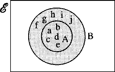
A ⊂ B is read as ‘A is a proper subset of B’ and means that A is a subset of B but A is not equal to B. Hence, A ⊂ B and simultaneously B ⊂ A are impossible.
A proper subset can be shown on a Venn diagram as in Figure 1.3.

1.3 Operations on sets
In Chapter 1 of the background Mathematics notes available on the companion website for this book, we study the rules obeyed by numbers when using operations like negation, multiplication, and addition. Sets can be combined in various ways using set operations. Sets and their operations form a Boolean Algebra which we look at in greater detail in Chapter 4, particularly its application to digital design. The most important set operations are as given in this section.
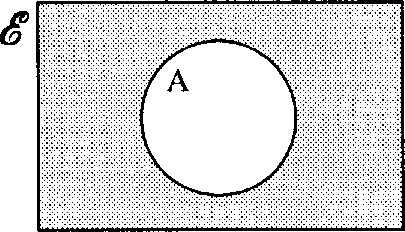
Complement
ˉA![]() or A' represents the complement of the set A. The complement of A is the set of everything in the universal set which is not in A, this is pictured in Figure 1.4.
or A' represents the complement of the set A. The complement of A is the set of everything in the universal set which is not in A, this is pictured in Figure 1.4.
Example 1.6
ɛ?=?ℕA?=?{x|x>5}then?A′?=?{1,2,3,4,5}
Example 1.7
The universal set is the set of real numbers represented by a real number line.
If A is the set of numbers less than 5, A = {x| x < 5} then A′ is the set of numbers greater than or equal to 5. A′ = {x| x ≥ 5}. These sets are shown in Figure 1.5.

Intersection
A ∩ B represents the intersection of the sets A and B. The intersection contains those elements that are in A and also in B, this can be represented as in Figure 1.6 and examples are given in Figures 1.7–1.10.


Note the following important points:
If A ⊆ B then A ∩ B = A. This is the situation in the example given in Figure 1.8.
If A and B have no elements in common then A ∩ B = Ø and they are called disjoint. This is the situation given in the example in Figure 1.9. Two sets which are known to be disjoint can be shown on the Venn diagram as in Figure 1.10.
Union
A ∪ B represents the union of A and B, that is, the set containing elements which are in A or B or in both A and B. On a Venn diagram, the union can be shown as in Figure 1.11 and examples are given in Figures 1.12–1.15.


Note the following important points:
If A⊆ B, then A ∪ B = B. This is the situation in the example given in Figure 1.13.
The union of any set with its complement gives the universal set, that is, A ∪ A′= ɛ, the universal set. This is pictured in Figure 1.15.
Cardinality of a finite set
The number of elements in a set is called the cardinality of the set and is written as n(A) or |A|.
Example 1.8
n(ϕ)?=?0,???????????n({2})?=?1,?????????n({a,b})?=2
![]()
For finite sets, the cardinality must be a natural number.
Example 1.9
In a survey, 100 people were students and 720 owned a video recorder; 794 people owned a video recorder or were students. How many students owned a video recorder?
E![]() = {x| x is a person included in the survey}
= {x| x is a person included in the survey}
Setting S = {x| x is a student} and V = {x| x owns a video recorder}, we can solve this problem using a Venn diagram as in Figure 1.16.

x is the number of students who own a video recorder. From the diagram we get
100−x+x+720−x=794?????????⇔??820−x?=?794?????????⇔??x?=?26
Therefore, 26 students own a video recorder.
1.4 Relations and functions
Relations
A relation is a way of pairing up members of two sets. This is just like the idea of family relations. For instance, a child can be paired with its mother, brothers can be paired with sisters, etc. A relation is such that it may not always be possible to find a suitable partner for each element in the first set whereas sometimes there will be more than one. For instance, if we try to pair every boy with his sister there will be some boys who have no sisters and some boys who have several. This is pictured in Figure 1.17.

Functions
Functions are relations where the pairing is always possible. Functions are like mathematical machines. For each input value there is always exactly one output value.
Calculators output function values. For instance, input 2 into a cal-culator, press 1/x and the calculator will display the number 0.5. The output value is called the image of the input value. The set of input values is called the domain and the set containing all the images is called the codomain.
The function y = 1/ x is displayed in Figure 1.18 using arrows to link input values with output values.

Functions can be represented by letters. If the function of the above example is given the letter f to represent it then we can write
f?:x↦1x
![]()
This can be read as ‘fis the function which when input a value for x gives the output value l/x’. Another way of giving the same information is:
f(x)?=?1x
![]()
f (x) represents the image of x under the function f and is read as ‘f of x’. It does not mean the same as f times x.
f(x) = l/x means ‘the image of x under the function f is given by 1/ x’ but is usually read as ‘f of x equals l/x′.
Even more simply, we usually use the letter y to represent the output value, the image, and x to represent the input value. The function is therefore summed up by y = 1/ x.
x is a variable because it can take any value from the set of values in the domain. y is also a variable but its value is fixed once x is known. So x is called the independent variable and y is called the dependent variable.
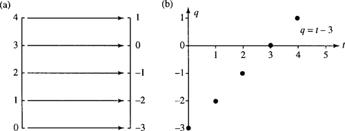
The letters used to define a function are not important. y = 1/x is the same as z = 1/t is the same as p = 1/q provided that the same input values (for x, t, or q) are allowed in each case.
More examples of functions are given in arrow diagrams in Figures 1.19(a) and 1.20(a). Functions are more usually drawn using a graph, rather than by using an arrow diagram. To get the graph the codomain is moved to be at right angles to the domain and input and output values are marked by a point at the position (x, y). Graphs are given in Figures 1.19(b) and 1.20(b).

Continuous functions and discrete functions applied to signals
Functions of particular interest to engineers are either functions of a real number or functions of an integer. The function given in Figure 1.19 is an example of a real function and the function given in Figure 1.20 is an example of a function of an integer, also called a discrete function.
Often, we are concerned with functions of time. A variable voltage source can be described by giving the voltage as it depends on time, as also can the current. Other examples are: the position of a moving robot arm, the extension or compression of car shock absorbers and the heat emission of a thermostatically controlled heating system. A voltage or current varying with time can be used to control instrumentation or to convey information. For this reason it is called a signal. Telecommunication signals may be radio waves or voltages along a transmission line or light signals along an optical fibre.
Time, t, can be represented by a real number, usually non-negative. Time is usually taken to be positive because it is measured from some reference instant, for example, when a circuit switch is closed. If time is used to describe relative events then it can make sense to refer to negative time. If lightning is seen 1 s before a thunderclap is heard then this can be described by saying the lightning happened at –1 s or alternatively that the thunderclap was heard at 1 s. In the two cases, the time origin has been chosen differently. If time is taken to be continuous and represented by a real variable then functions of time will be continuous or piecewise continuous. Examples of graphs of such functions are given in Figure 1.21.

A continuous function is one whose graph can be drawn without taking your pen off the paper. A piecewise continuous function has continuous bits with a limited number of jumps. In Figure 1.21, (a) and (b) are continuous functions and (c) is a piecewise continuous function. If we have a digital signal, then its values are only known at discrete moments of time. Digital signals can be obtained by using an analog to digital (A/D) convertor on an originally continuous signal. Digital signals are represented by discrete functions as in Figure 1.22(a)–(c)

A digital signal has a sampling interval, T, which is the length of time between successive values. A digital functions is represented by a discrete function. For example, in Figure 1.22(a) the digital ramp can be represented by the numbers
0,1,2,3,4,5,…
![]()
If the sample interval T is different from 1 then the values would be
0,T,2T,3T,4T,5T,…
![]()
This is a discrete function also called a sequence. It can be represented by the expression f(t) = t, where t = 0,1,2,3,4,5,6, … or using the sampling interval, T, g(n) = nT, where n = 0, 1,2,3,4,5,6, …
Yet another common way of representing a sequence is by using a subscript on the letter representing the image, giving
fn?=?n,??where?n?=?0,1,2,3,4,5,…
![]()
or, using the letter a for the image values,
an?=?n,?where?n?=?0,1,2,3,4,5,…
![]()
Substituting some values for n into the above gives
a0?=?0,?a1?=1,?a2?=2,?a3?=?3,…
![]()
As a sequence is a function of the natural numbers and zero (or if negative input values are allowed, the integers) there is no need to specify the input values and it is possible merely to list the output values in order. Hence the ramp function can be expressed by 0, 1,2,3,4,5,6, …
Time sequences are often referred to as ‘series’. This terminology is not usual in mathematics books, however, as the description ‘series’ is reserved for describing the sum of a sequence. Sequences and series are dealt with in more detail in Chapter 18.
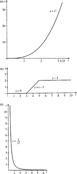
Example 1.10
Plot the following analog signals over the values of t given (t real):
x?=?t3??????t≥0
![]()
(b)
y?={0t≤3t−33<t≤52t>5
(c)
z?=?1t2??????t>0
![]()
Solution In each case, choose some values of t and calculate the function values at those points. Plot the points and join them.
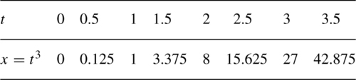
These values are plotted in Figure 1.23(a).
(a)x=t3???t≥?0(b)y={0t≤3t-33<t≤52t>5(c)z=1/t2??t>0

(b)
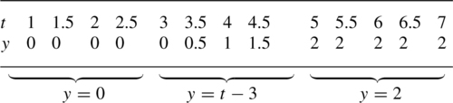
These values are plotted in Figure 1.23(b).
(c)

These values are plotted in Figure 1.23(c).
Example 1.11
Plot the following discrete signals over the values of t given (t an integer):
x?=?1t−1??t>2
![]()
(b)
y?=?{0t≤41/t−0.254<t<10−0.15t≥10
(c)
z?=?4t−2??t>0
![]()
Solution In each case, choose successive values of t and calculate the function values at those points. Mark the points with a dot.

These values are plotted in Figure 1.24(a).

(a)x=1t-1??t>2???(b)y={0t≤41/t-0.254<t<10??(c)z=4t-2??t>0-0.15t≥10

(b)

These values are plotted in Figure 1.24(b).
(c)

These values are plotted in Figure 1.24(c).
Undefined function values
Some functions have ‘undefined values’, that is, numbers that cannot be input into them successfully. For instance input 0 on a calculator and try getting the value of 1/x. The calculator complains (usually displaying ‘-E- ’) indicating that an error has occurred. The reason that this is an error is that we are trying to find the value of 1/0 that is 1 divided by 0. Look at Chapter 1 of the Background Mathematics Notes, given on the accompanying website for this book, for a discussion about why division by 0 is not defined. The number 0 cannot be included in the domain of the function f (x) = 1/ x. This can be expressed by saying
f(x)?=?1/x,??????where?x∈ℝ?and?x?≠0
![]()
which is read as ‘f of x equals 1/x, where x is a real number not equal to 0'.
Often, we assume that we are considering functions of a real variable and only need to indicate the values that are not allowed as inputs for the function. So we may write
f(x)?=?1/x??????where?x≠0
![]()
Things to look out for as values that are not allowed as function inputs are:
1. Numbers that would lead to an attempt to divide by zero
2. Numbers that would lead to negative square roots
3. Numbers that would lead to negative inputs to a logarithm.
Examples 1.12(a) and (b) require solutions to inequalities which we shall discuss in greater detail in Chapter 2. Here, we shall only look at simple examples and use the same rules as used for solving equations. We can find equivalent inequalities by doing the same thing to both sides, with the extra rule that, for the moment, we avoid multiplication or division by a negative number.
Example 1.12
Find the values that cannot be input to the following functions, where the independent variable (x or r) is real:
y?=?3√x−2+5
![]()
(b)
y?=?3?log10(2−4x)
![]()
R?=r+10001000(r−2)
Solution
(a)?????y?=?3√x−2+5
![]()
Here x – 2 cannot be negative as we need to take the square root of it.
x−2≥0⇔x≥2
![]()
therefore, the function is
y?=?3√x−2+5??where?x≥2
![]()
(b)?????y?=?3?log10(2−4x).
![]()
Here 2 – 4x cannot be 0 or negative else we could not take the logarithm.
2−4x>0???⇔???2>4x???⇔???2/4>x
![]()
or?equivalently,?x??<12.?So?the?function?is
![]()
y?=?3?log10(2−4x)?????where?x?<0.5
![]()
(c)?????R?=?r+10001000(r−2)

Here 1000(r – 2) cannot be 0, else we would be trying to divide by 0. Solve the equation for the values that r cannot take
1000(r−2)=0r−2=0r=2
The function is
R?=?r+10001000(r−2)?????????where?r≠2
Example 1.13
Find the values that can be input to the following discrete functions where the independent variable is an integer
y?=?1k−4?????where?K?∈ℤ
![]()
(b)
f(k)?=?1(k−3)(k−2.2)?????where?k∈ℤ
(c)
an?=?n2??????where?n∈ℤ
![]()
Solution
(a)?????y?=?1k−4
![]()
Here k – 4 cannot be 0 else there would be an attempt to divide by 0. We get k – 4 = 0 when k = 4 so the function is:
y?=?1k−4?where?k≠4?and?k∈ℤ
![]()
(b)?????f(k)?=?1(k−3)(K−2.2)????where?k?∈ℤ
Solve for (k – 3) (k – 2.2) = 0 giving k = 3 or k = 2.2. As 2.2 is not an integer then there is not need to specifically exclude it from the function input values, so the function is
f(k)?=?1(k−3)(k−2.2)????where?k≠3?and?k∈ℤ

(c)?????an?=?n2,?????n∈ℤ
![]()
Here there are no problems with the function as any integer can be squared. There are no excluded values from the input of the function.
Using a recurrence relation to define a discrete function
Values in a discrete function can also be described in terms of its values for preceeding integers.
Example 1.14
Find a table of values for the function defined by the recurrence relation:
f(n)?=?f(n−1)+2
where f(0) = 0.
Solution Assuming that the function is defined for n = 0, 1, 2, … then we can take successive values of n and find the values taken by the function. n = 0 givesf (0) = 0 as given.
Substituting n = 1 into Equation (1.1) gives
f(1)?=?f(1−1)+2???????⇔?????f(1)=f(0)+2=0+2=2(using?f(0)=0)

hence, f(l) = 2.
Substituting n = 2 into Equation (1.1) gives
f(2)?=?f(2−1)+2⇔f(2)?=?f(1)+2⇔f(2)?=f(1)+2=2+2=4(using?f(1)=2)

hence, f(2) = 4.
Substituting n = 3 into Equation (1.1) gives
f(3)?=?f(3−1)+2???⇔f(3)?=?f(2)+2=4+2(using?f(2)=4)

hence, f(3) = 6.
Continuing in the same manner gives the following table:

Notice we have filled in the general term f(n) = 2n. This was found in this case by simple guess work.
1.5 Combining functions
The sum, difference, product, and quotient of two functions, f and g
Two functions with ![]() as their domain and codomain can be combined using arithmetic operations. We can define the sum of f and g by
as their domain and codomain can be combined using arithmetic operations. We can define the sum of f and g by
(f+g):x↦f(x)+g(x)
![]()
The other operations are defined as follows:
(f−g):x↦f(x)−g(x)???difference,(f×g):x↦f(x)×g(x)????product,(f/g):x↦f(x)g(x)???quotient.

Example 1.15
Find the sum, difference, product, and quotient of the functions:
f?:x↦x2?and?g:x↦x6
![]()
Solution
(f+g):x↦x2+x6(f−g):x↦x2−x6(f×g):x↦x2×x6=x8(f/g):x↦x2x6?=x−4
The specification of the domain of the quotient is not straightforward. This is because of the difficulty which occurs when g(x) = 0. When g(x) = 0 the quotient function is undefined and we must remove such elements from its domain. The domain of f/g is ![]() with the values where g (x) = 0 omitted.
with the values where g (x) = 0 omitted.
Composition of functions
This method of combining functions is fundamentally different from the arithmetical combinations of the previous section. The composition of two functions is the action of performing one function followed by the other, that is, a function of a function.
Example 1.16
A post office worker has a scale expressed in kilograms which gives the cost of a parcel depending on its weight. He also has an approximate formula for conversion from pounds (lbs) to kilograms. He wishes to find out the cost of a parcel which weighs 3 lb.
The two functions involved are:
a:?kilograms→?money?and?c:?1bs→kilogramsa?is?defined?by?Figure?1.25?and?the?function?c?is?given?byc?:?x?↦x/2.2

Solution The composition ‘a o c’ will be a function from lbs to money.
Hence, 3 lb after the function c gives 1.364 and 1.364 after the function a gives €1.90 and therefore
(a?o?c)(3)?=?€1.90.
![]()
Example 1.17
Supposing f (x) = 2x + 1 and g (x) = x2, then we can combine the functions in two ways.
1. A composite function can be formed by performing f first and then g, that is, g o f. To describe this function, we want to find what happens
to x under the function g o f. Another way of saying that is we need to find g(f(x)). To do this call f(x)a new letter, say y.
y?=?f(x)?=?2x+1
Rewrite g as a function of y
g(y)?=?y2
![]()
Now substitute y = 2x + 1 giving
g(2x+1)?=?(2x+1)2
![]()
Hence,
g(f(x))?=?(2x+1)2(g?o?f)(x)?=?(2x+1)2.
2. A composite function can be formed by performing g first and then f, that is, f o g. To describe this function, we want to find what happens to x under the function f o g. Another way of saying that is we need to find f (g(x)). To do this call g (x)a new letter, say y.
y=g(x)=x2
![]()
Rewrite f as a function of y
f(y)=2y+1
![]()
Now substitute y = x2giving
f(x2)=2x2+1
![]()
Hence,
f(g(x))=2x2+1(f?o?g)(x)=2x2+1.
Example 1.18
Supposing u (t) = 1/(t – 2) and v (t) = 3 – t then, again, we can combine the functions in two ways.
1. A composite function can be formed by performing u first and then v, that is, v o u. To describe this function, we want to find what happens to t under the function v o u. Another way of saying that is we need to find v (u (t)). To do this call u (t)a new letter, say y.
y?=?u(t)?=?1t−2
![]()
Rewrite v as a function of y
ν(y)?=?3−y
![]()
Now substitute y = 1/(t – 2) giving
ν(1t−2)?=?3−1t−2=3(t−2)−1t−2(rewriting?the?expression?over?a?common?denominator)=3t−6−1t−2?=?3t−7t−2

Hence,
ν(u(t))?=?3t−7t−2(ν?o?u)(t)??=?3t−7t−2

2. A composite function can be formed by performing v first and then u, that is u o v. To describe this function, we want to find what happens to t under the function u o v. Another way of saying that is we need to find u (v (t)). To find this call v (t)a new letter, say y.
y=v(t)=3-t
![]()
Rewrite u as a function of y
u(y)?=?1y−2
Now substitute y = 3 – t giving
ν(3−t)?=?1(3−t)−2?=?11−t
Hence,
u(ν?(t))=11−t(u?o?ν)(t)?=?11−t
Decomposing functions
In order to calculate the value of a function, either by hand or using a calculator, we need to understand how it decomposes. That is we need to understand to order of the operations in the function expression
Example 1.19
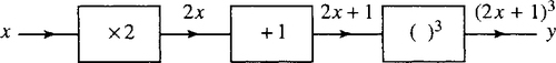
Calculate y = (2x + 1)3 when x = 2
Solution Remember the order of operations discussed in Chapter 1 of the Background Mathematics booklet available on the companion website. The operations are performed in the following order: Start with x = 2 then
2x?=?42x+1=5(2x+1)3?=?125

So, there are three operations involved
2. add on 1,
3. take the cube.
This way of breaking down functions can be pictured using boxes to represent each operation that makes up the function, as was used to represent equations in Chapter 3 of the Background Mathematics booklet available on the companion website. The whole function can be thought of as a machine, represented by a box. For each value x, from the domain of the function that enters the machine, there is a resulting image, y, which comes out of it. This is pictured in Figure 1.26.

Inside of the box, we can write the name of the functions or the expression which gives the function rule. A composite function box can be broken into different stages, each represented by its own box. The function y = (2x + 1)3 breaks down as in Figure 1.27.
y = (3x – 4)4 can be broken down as in Figure 1.28.

The inverse of a function
The inverse of a function is a function which will take the image under the function back to its original value. If f−l(x) is the inverse of f(x) then
f−1(f(x))?=?x(f−1?o?f):x↦x
Example 1.20
f(x)?=?2x+1f−1(x)?=x−12

To show this is true, look at the combined function f−1 (f (x)) = (2x + 1 – 1)/2 = x.
Finding the inverse of a linear function
One simple way of finding the inverse of a linear function is to:
1. Decompose the operations of the function.
2. Combine the inverse operations (performed in the reverse order) to give the inverse function.
This is a method similar to that used to solve linear equations in Chapter 3 of the Background Mathematics Notes available on the companion website for this book.
Example 1.21
Find the inverse of the function f (x) = 5x – 2.
The method of solution is given in Figure 1.29.
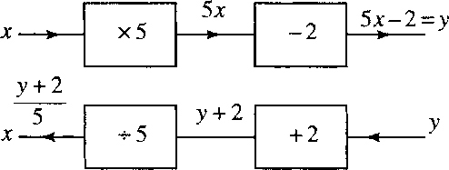
The inverse operations give that x = (y + 2)/5. Here y is the input value into the inverse function and x is the output value. To use x and y in the more usual way, where x is the input and y the output, swap the letters giving the inverse function as
y=x+25
![]()
This result can be achieved more quickly by rearranging the expression so that x is the subject of the formula and then swap x and y.
Example 1.22
Find the inverse of f (x) = 5x – 2.
y=5x−2⇔???y+2=5x⇔???y+25?=?x⇔???x=y+25

Now swap x and y to give y = (x + 2)/5. Therefore,
f−1(x)=(x+2)/5.
![]()
Example 1.23
Find the inverse of
g(x)=12−x??????where?x≠2
![]()
Set
y=12−x?⇔??y(2−x)?=1⇔2y−xy=1⇔2y=1+xy⇔2y−1=xy⇔xy=2y−1⇔x=2y−1y??????where?y≠0⇔x=2−1y

Swap x and y to give y = 2 – (1/x)
So
g−1(x)?=?2−1x????x≠0
![]()
To check, try a couple of values of x.
Try x = 4,
g(x)=12−x?=?12−4?=?−12
![]()
Perform g−l on the output value –(1/2).
Substitute g(4) = –(1/2) into g−l(x):
g−1(−12)?=?2−1−(1/2)?=?2+2=4.

The function followed by its inverse has given us the original value of x.
The range of a function
When combining functions, for example, f(g(x)), we have to ensure that g (x) will only output values that are allowed to be input to f. The set of images of g(x) becomes an important consideration. The set of images of a function is called its range. The range of a function is a subset of its codomain.
1.6 Summary
1. Functions are used to express relationships between physical quantities.
2. The allowed inputs to a function are grouped into a set, called the domain of the function. The set including all the outputs is called the codomain.
3. A set is a collection of objects called elements.
4. ɛ is the universal set, the set of all objects we are interested in.
5. ϕ is the empty set, the set with no elements.
6. The three most important operations on sets are:
(a) intersection: A ∩ B is the set containing every element in both A and B;
(b) union: A ∪ B is the set of elements in A or in B or both;
(c) complement: A' is the set of everything, in the universal set, not in A.
7. A relation is a way of pairing members of two sets.
8. Functions are a special type of relation which can be thought of as mathematical machines. For each input value there is exactly one output value.
9. Many functions of interest are functions of time, used to represent signals. Analogue signals can be represented by functions of a real variable and digital signals by functions of an integer (discrete functions). Functions of an integer are also called sequences and can be defined using a recurrence relation.
10. To find the domain of a real or discrete function exclude values that could lead to a division by zero, negative square roots, or negative logarithms or other undefined values.
11. Functions can be combined in various ways including sum, difference, product, and quotient. A special operation of functions is composition. A composite function is found by performing a second function on the result of the first.
12. The inverse of a function is a function which will take the image under the function back to its original value.
1.7 Exercises
1.1 Given ɛ = {a, b, c, d, e, f, g}, A = {a, b, e}, B = {b, c, d, f},C = {c, d, e}.
Write down the following sets:
(b) A ∪ B
(c) A ∩ C′
(d) (A ∪ B) ∩ C
(e) (A ∩ C) ∪ (B ∩ C)
(f) (A ∩ B) ∪ C
(g) (A ∪ C) ∩ (B ∪ C)
(h) (A ∩C)′
(i) A′ ∪ C'.
1.2. Use Venn diagrams to show that:
(b) (A ∪ B) ∪ C = A ∪ (B ∪ C)
(c) (A ∩ B) ∪ C = (A ∪ C) ∩ (B ∪ C)
(d) (A ∪ B) ∩C = (A ∩ C) ∪ (B ∩C)
(e) (A ∩B)′ = A′ ∪ B′
(f) (A ∪ B)'=A' ∩ B'.
1.3. Let ɛ = {0, 1, 2, 3, 4, 5, 6, 7, 8, 9} and given P = {x | x < 5}, Q = {x|x ≥ 3} find explicitly:
(b) Q
(c) P ∪ Q
(d) P′
(e) P'∩ Q.
1.4. Below are various assertions for any sets A and B. Write true or false for each statement and give a counter-example if you think the statement is false.
(b) (A ∩ B)′ ⊆ A
(c) A ∩ B = B∩ A
(d) A ∩ B′ = B ∩ A′.
1.5. Using a Venn diagram simplify the following:
(b) A ∪ (B ∩ A′)
(c) A ∩ (B ∪ A′).
1.6. A computer screen has 80 columns and 25 rows:
(a) Define the set of positions on the screen.
(b) Taking the origin as the top left hand corner define:
(i) the set of positions in the lower half of the screen as shown in Figure 1.30(a);

(ii) the set of positions lying on or below the diagonal as shown in Figure 1.30(b).
1.7. A certain computer system breaks down in two main ways: faults on the network and power supply faults. Of the last 50 breakdowns, 42 involved network faults and 20 power failures. In 13 cases, both the power supply and the network were faulty. How many breakdowns were attributable to other kinds of failure?
1.8. Draw arrow diagrams and graphs of the following functions:
(a) f(t) = (t –1)2 t ∈{0, 1, 2, 3, 4}
(b) g(z) = l/z z ∈ {–1, −0.5, 0.5, 1, 1.5, 2}
(c)
y={xx∈{−2,?−1}2xx∈{0,1,2,3}
(d) h : t ![]() 3 – t t ∈{5,6,7,8,9,10}
3 – t t ∈{5,6,7,8,9,10}
1.9. Given that f : x ![]() 2x −1, g: x
2x −1, g: x ![]() (1/3)x2, h : x
(1/3)x2, h : x ![]() 3/x
3/x
(ii) g (3)
(iii) h (5)
(iv) h (2) + g(2)
(v) h/g (5)
(vi) (h × g)(2)
(vii) h(g(2))
(viii) h(h(3))
(b) Find the following functions:
(ii) g ![]() f
f
(iii) h ![]() g
g
(iv) f−1
(v) h−1
(c) Confirm the following:
(ii) (h−1 ![]() h): x
h): x ![]() x
x
(iii) (f ![]() f−1): x
f−1): x ![]() x
x
(d) Using the results from sections (b) and (c), find the following:
(ii) h(g(5))
(iii) g(f(4))
1.10. An analog signal is sampled using an A/D convertor and represented using only integer values. The original signal is represented by g(t) and the digital signal by h(t) sampled at t ∈{2,3,4,5,6,7,8,9,10}. The definitions of g and h are as below
g(t)={t−2.25t<56.8−tt≥5

h:2↦0h:3↦1h:4↦2h:5↦2h:6↦1h:7↦0h:8↦−1h:9↦−2h:10↦−3

If e(t)is the error function (called quantization error), defined at the sample points, find e(t) and represent it on a graph.