17.1 Introduction

We concentrated so far in this book on functions of time. In Chapter 5 we looked at waves that were functions of distance, x, and time, t. For many applications, we need to analyse functions of the three possible spatial coordinates, x, y, and z and also of time, t. For instance, consider making a mug of tea using a tea bag. When first brewed, the temperature will be nearly at boiling point 100°C. The temperature of the water will start off being much the same everywhere but it will be cooler near the tea bag and at the sides of the mug. As time progresses the surface of the tea and those parts in touch with the mug, will cool quicker than the centre of the tea. We can see that the temperature of a mug of tea is a function both of where in the mug we measure it and also the length of time since the tea was first made. This is a function of more than one variable.

Some of the ideas that we have learnt for analysing a function of a single variable we revisit here for functions of more than one variable. In this chapter we consider graphs of functions and taking their partial derivatives, changing variables, using the chain rule and the derivative in any given direction. To begin we need to think about visualizing these functions and that means considering how to visualize graphs of functions that would require three or more dimensions when armed only with a two-dimensional sheet of paper.

17.2 Functions of two variables – surfaces

When drawing a graph we need one dimension to represent the actual function value, the dependent variable, for which we have used the vertical axis. When drawing a graph of distance, x or of time t, we are able to use the horizontal axis of the graph to represent the independent variable. Supposing now we have a function of two spatial dimensions – for instance, the height above sea level on a landscape or the temperature in a cup of tea at the surface of the tea. We would like to be able to picture these functions. However, we need more than one horizontal axis in order to be able to represent the spatial dimensions x and y when a picture on a page of this book has only one horizontal direction. We could build three-dimensional models only this would be time consuming and make book production even more costly. One of the ways of representing these graphs on a page of paper is to use a perspective representation of a surface. The other way of doing it is to draw a plan of the function from above and use contours to represent the function value at each point. You are familiar with this from maps that mark contours representing the height of the ground at each point. Another example is meteorological forecasts that use contours superimposed on maps of the country, to represent the air pressure. A third way to picture the functions is to take a cross section parallel to either one of the x- or y-axes.

Graphs of functions of two variables

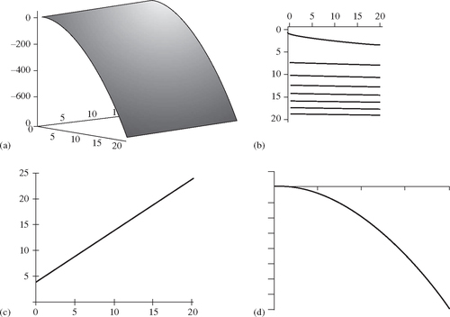
The function:

$\varphi =\frac{4\pi {\varepsilon }_{0}q}{{(x^2+y^2)}^{1/2}}$

represents the electrical potential field of a point source (where z = 0) positioned at the origin. Various graphs of this function are shown in Figure 17.1: (a) has a perspective view; (b) has a contour representation; and (c) and (d) show x and y cross-sections.

Graphs of the function h = 4 −2x² + y are shown in Figure 17.2.

17.3 Partial differentiation

From the graphs of functions that we looked at in the last section we can see that we are able to take a cross-section either parallel to the x-axis or parallel to the y-axis. Each cross-section can be represented by a function of one variable only. If we take a cross-section parallel to the x-axis, then we have fixed y and only x is varying. In this case, we can differentiate the function as a function of one variable.

It is this idea that is used for partial differentiation. We can find the derivative along a line parallel to the x-axis by ‘freezing’ y and differentiation with respect to x only. We can find the derivative along a line parallel to the y-axis by ‘freezing’ x and differentiation with respect to y only. Partial derivatives of the function u = f (x, y) are defined by:

$\frac{\partial u}{\partial x}=\underset{\delta x\to 0}{lim}\frac{u(x+\delta x,y)-u(x,y)}{\delta x}$

$\frac{\partial u}{\partial y}=\underset{\delta y\to 0}{lim}\frac{u(x,y+\delta y)-u(x,y)}{\delta y}$

∂u/∂x reads as ‘partial du by dx’ and ∂u/∂y reads as ‘partial du by dy’.

17.4 Changing variables – the chain rule

Supposing we have a function, u = f(x, y), and x and y are functions of s and t so that x = v(s,t),y = w(s,t), and u = F(s,t). We want to find a relationship between the partial derivatives of u with respect to s and t and those with respect to x and y. We assume in the following discussion that we have well-behaved functions, that is, the functions and their partial derivatives do not have discontinuities in the region of x, y.

We want to find the partial derivative of u with respect to s, that is, we would like to find

$\frac{\partial u}{\partial s}=\underset{\delta s\to 0}{lim}\frac{u(s+\delta s,t)-u(s,t)}{\delta s}.$

As we are considering a change of variable so that the point (x, y) corresponds to the point (s, t) and therefore u (x, y) = u (s, t). We consider a small change, δs, in the variable s so that the point (s + δs, t) will correspond to some point (x + δx, y + y) in the (x, y) plane, where δx and δy are small. Again u(s + δs, t) will have the same value as u(x + δx,y + δy). Using u(s + δs,t) = u(x + δy,y + δy) = u(x + δx,y + δy) – u(x,x + δy) + u(x,y + δy) and u(x,y) = u(s, t) we find:

$\begin{array}{l}\frac{\partial u}{\partial s}=\underset{\delta s\to 0}{lim}\frac{u(x+\delta x,y?+\delta y)-u(x,y+\delta y)+u(x,y+\delta y)-u(x,y)}{\delta s}\\ =\underset{\delta s\to 0}{lim}\frac{u(x+\delta x,y+\delta y)-u(x,y+\delta y)}{\delta s}\\ +\underset{\delta s\to 0}{lim}\frac{u(x,y+\delta y)-u(x,y)}{\delta s}.\end{array}$

As long as δx, δy are not actually equal to 0 we can multiply the first term by δx /δx and the second term by δy /δy. As 8s →0, so also δx → 0 and δy → 0, hence we get

$\begin{array}{l}\frac{\partial u}{\partial s}=\underset{\delta x\to 0,\delta y\to 0}{lim}\frac{u(x+\delta x,y?+\delta y)-u(x,y+\delta y)}{\delta x}\underset{\delta s\to 0}{lim}\frac{\delta x}{\delta s}\\ +\underset{\delta x\to 0}{lim}\underset{\delta y\to 0}{lim}\frac{u(x,y+\delta y)-u(x,y)}{\delta y}\underset{\delta s\to 0}{lim}\frac{\delta y}{\delta s}.\end{array}$

In the first term, we can take the limit as δy → 0 to get:

$\begin{array}{l}\frac{\partial u}{\partial s}=\underset{\delta x\to 0}{lim}\frac{u(x+\delta x,y)-u(x,y)}{\delta x}\underset{\delta s\to 0}{lim}\frac{\delta x}{\delta s}\\ +\underset{\delta y\to 0}{lim}\frac{u(x,y+\delta y)-u(x,y)}{\delta y}\underset{\delta s\to 0}{lim}\frac{\delta y}{\delta s}.\end{array}$

Using our previous definitions of the partial derivative we take the limits to find:

$\frac{\partial u}{\partial s}=\frac{\partial u}{\partial x}\frac{\partial x}{\partial s}+\frac{\partial u}{\partial y}\frac{\partial y}{\partial s}.$

Similarly, we can show that

$\frac{\partial u}{\partial t}=\frac{\partial u}{\partial x}\frac{\partial x}{\partial t}+\frac{\partial u}{\partial y}\frac{\partial y}{\partial t}.$

17.5 The total derivative along a path

We have found the derivatives in the x- and y-directions for some function u = f (x, y). We would now like to consider the derivative along any given path, where for instance x = g(t) and y = h(t), that is, both x and y are a function of t. Consider a small change in u, δu, in the direction of the path, with a change in t of δt. Then we can define the total derivative along the path as:

$\frac{du}{dt}=\underset{\delta t\to 0}{lim}\frac{u(x+\delta x,y+\delta y)-u(x,y)}{\delta t}\mathrm{.}$

Substituting u(x + δy, y + δy) = u(x + δx, y + δy) − u(x,x + δy) + u(x, y + δy) and multiplying the first term by δx /δx and the second term by δy /δy gives:

$\begin{array}{l}\frac{\text{d}u}{\text{d}t}=\underset{\delta x\to 0,\delta y\to 0}{lim}\frac{u(x+\delta x,y?+\delta y)-u(x,y+\delta y)}{\delta x}\underset{\delta t\to 0}{lim}\frac{\delta x}{\delta t}\\ +\underset{\delta x\to \mathrm{0,}}{lim}\underset{\delta y\to 0}{lim}\frac{u(x,y+\delta y)-u(x,y)}{\delta y}\underset{\delta t\to 0}{lim}\frac{\delta y}{\delta t}.\end{array}$

As x and y are functions of t only,

$\underset{\delta t\to 0}{lim}\frac{\delta x}{\delta t}=\frac{\text{d}x}{\text{d}t}\text{and}\underset{\delta t\to 0}{lim}\frac{\delta y}{\delta t}=\frac{\text{d}x}{\text{d}t}$

so taking the limits in the expression above we get:

$\frac{\text{d}u}{\text{d}t}=\frac{\partial u}{\partial x}\frac{\text{d}x}{\text{d}t}+\frac{\partial u}{\partial y}\frac{\text{d}y}{\text{d}t}.$

This is the second version of the chain rule, where we are not just making a change of variables but now we are limiting the direction of the derivative to be along a particular path, such that x = g(t) and y = h(t). This is the total derivative function along the path and du/dt is the gradient of the tangent along the path defined by (x(t), y(t)).

17.6 Higher-order partial derivatives

We can carry on differentiating partial derivatives to find higher-order partial derivatives such as ∂²u/∂x², ∂²u/∂y², ∂²u/∂x∂y and ∂²u/∂y∂x, where

$\begin{array}{l}\frac{{\partial }^{2}u}{\partial x^2}=\frac{\partial }{\partial x}\frac{\partial u}{\partial x}\\ \frac{{\partial }^{2}u}{\partial y^2}=\frac{\partial }{\partial y}\frac{\partial u}{\partial y}\\ \frac{{\partial }^{2}u}{\partial x\partial y}=\frac{\partial }{\partial x}\frac{\partial u}{\partial y}\\ \frac{{\partial }^{2}u}{\partial y\partial x}=\frac{\partial }{\partial y}\frac{\partial u}{\partial x}.\end{array}$

For functions with continuous first-order derivatives

$\frac{{\partial }^{2}u}{\partial x\partial y}=\frac{{\partial }^{2}u}{\partial y\partial x}.$

The partial derivatives ∂²u/∂x², ∂²u/∂y², ∂²u/∂x∂y, and ∂²u/∂y∂x are called the second-order partial derivatives of u because we have differentiated twice to find them. We can continue differentiating to find third-and higher-order partial derivatives.

17.7 Summary

1. A function u (x, y) is a function of two variables x and y; u is the dependent variable and x and y are the independent variables. The graph of this function can be represented on the page of a book or a computer screen by using a perspective representation of a surface or by using contours to represent the lines where the value of the function is constant.

2. A Function of two variables f(x y) has two first-order partial derivatives. The partial derivative with respect to x is found by considering y to be constant and then differentiating with respect to x only. The partial derivative with respect to y is found by considering x to be a constant and differentiating with respect to y only.

3. The chain rule can be used to change the variables of differentiation. Supposing we have a function, u = f(x, y), and x and y are functions of s and t so that x = v(s, t), y = w(s, t), and u = F(s, t), then:

$\frac{\partial u}{\partial s}=\frac{\partial u}{\partial x}\frac{\partial x}{\partial s}+\frac{\partial u}{\partial y}\frac{\partial y}{\partial s}\text{and}\frac{\partial u}{\partial t}=\frac{\partial u}{\partial x}\frac{\partial x}{\partial t}+\frac{\partial u}{\partial y}\frac{\partial y}{\partial t}$

4.  If we know the path on which we are travelling across the surface f (x, y), so that x and y are defined in terms of a parameter t, then it is possible to find the total derivative of f with respect to t because the gradient along the path will be unique at each point. It this case we can use:

$\frac{\text{d}u}{\text{d}t}=\frac{\partial u}{\partial x}\frac{\text{d}x}{\text{d}t}+\frac{\partial u}{\partial y}\frac{\text{d}y}{\text{d}t}.$

5. Partial derivatives can be used for approximating the value of a function near a known value. For a function of two variables we have:

$\delta u\approx \frac{\partial u}{\partial x}\delta x+\frac{\partial u}{\partial y}\delta y.$

This can also be used to estimate the maximum error in a calculated value.

17.8 Exercises

17.1 Find the first-order partial derivatives of the following:

(a) $f\left(x,?y\right)=x?\text{ln}\left(y^2\right)$

(b) $g\left(x,?y\right)=x?+?xy-\frac{\text{4x}}{\text{y}}$

(c) $h\left(x,?y\right)=?{tan}^{-1}\left(\frac{x}{y}\right)$

(d) $f\left(x,?y\right)=?\frac{4x}{y}{\text{e}}^{-x^2}.$

17.2 Use the chain rule to find partial derivatives of the following in terms of x and y where $r=\sqrt{x^2+y^2}$ and $\theta ={tan}^{-1}\left(\frac{y}{x}\right)$.

(a) u (r, θ) = sin(θ)/r

(b) u (r,θ) = r² + tan (θ).

17.3 Given $u=\left(x^2+y^2\right)/\sqrt{y}$, find the value of the following partial derivatives at the point (0,4)

(a) $\frac{\partial u}{\partial y}$

(b) $\frac{{\partial }^{2}u}{{\partial }_x{\partial }_y}$

(c) $\frac{{\partial }^{2}u}{{\partial }_y{\partial }_x}$

(d) $\frac{{\partial }^{2}u}{\partial x^2}$

(e) $\frac{{\partial }^{2}u}{\partial y^2}$.

17.4 Given z = x² + y² and x = r cos(θ), y = r cos(θ) find ∂z/∂r and ∂z/∂θ by substitution and by using the relationships between the partial derivatives. Show that the results obtained are equal.

17.5 Given that z = 2x + 3y² and x = 3t> + 5,y = − 2t find $\partial z/\partial x,?\partial z/\partial y,?\text{d}x/\text{d}t,?\text{d}y/\text{d}t,?\text{and}?\text{d}z/\text{d}t$.

17.6 Given u = e^−8t(A cos(2x) + B sin(2x)), evaluate $\partial u/\partial t$ and ${\partial }^{2}u/\partial x^2$ and hence show that u is a solution to the partial differential equation $\partial u/\partial t=2{\partial }^{2}u/\partial x^2$.

17.7 Use the approximation

$\delta u\approx \frac{\partial u}{\partial x}\delta x+\frac{\partial u}{\partial y}\delta y$

with $u=\sqrt{x^2+y^3}$ near the point (6,4) to estimate the value of $\sqrt{{5.96}^2+{4.03}^3}$.

17.8 The power delivered to the load resistance R_L for the circuit is given by

$P=25?R_L/{\left(R+R_L\right)}^2$

If R = 2000 and R_L = 1000 with a possible error of 5% in either, find P and estimate the maximum error in P.

17.9 The height, width, and length of an open box are subject to errors of 1, 2, and 3%, respectively. Estimate to the nearest percentage the maximum relative error in calculating the surface area of the box for a desired height of 4 m, width of 3 m, and length of 2 m.