
13.5 Gauss elimination
Gauss elimination is a structured process for the elimination of variables in one of the equations. It is easy to generalize to larger systems of equations and it is relatively numerically stable, making it suitable for use with a computer.
Gauss elimination is performed in stages. At Stage 1, we concentrate on the first column, the coefficients of x. The idea is to make the coefficient of the first equation 1 and eliminate the variable from the other equation(s) by using multiples of the first equation. Equation 1 is therefore the pivotal equation for Stage 1.
Example 13.25
Solve
3x+4y=75x−8y=8

using Gauss elimination.
Solution We can either write out the equation each time we perform a step or we can abbreviate the solution by expressing the equations in short hand as an augmented matrix
(3475−88).

We shall present both notations at the same time. We shall refer to the elements in the augmented matrix by
(a11a12b1a21a22b2).
For the first step, the first equation is the pivotal equation:
3x+4y=75x−8y=8?(3475−88).
Stage 1
Step 1: Divide the first equation by a11:
x+43y=735x−8y=8?(143735−88).

Step 2: Take 5 times the first equation away from the second equation in order to eliminate the term in x in the second equation:
x+43y=73? −8y−(43y×5)=8−73×5

which is the same as
x+43y=73? −443y=−113(143730−443−113).

Stage 2:
Divide the second equation through by the coefficient of y(a22).
x+43y=73 y=14(143730114).
We now already have the solution for y and we can obtain the solution for x by substitution into the first equation. This is called ‘back-substitution’.
x+(43)(14)=73?⇔?x=73−13?⇔?x=2.

Therefore, the solution is (2, 0.25).
We see that the point of the exercise is to write the system of equations so that the final equation contains only one variable and the last but one equation has up to two variables, etc. The matrix of coefficients should be in upper triangular form like:
(14301).

The augmented matrix is then like

which is said to be in echelon form. Once this form has been achieved, then back-substitution can be performed to find the value of the variables.
Example 13.26
Solve the system of equations
2x+y−2z=−12x−3y+2z=9−?x+y−z=−3.5.
Solution
2x+y−2z=−12x−3y+2z=9−x+y−z=−3.5(21−2−12−329−11−1−3.5).
Stage 1
Stage 1 concerns the first column. We use the first row (the pivotal row) to eliminate the elements below a11.
Step 1: Divide the first equation by a11.
x+0.5y−z=−0.52x−3y+2z=9−x+y−z=−3.5(10.5−1−0.52−329−11−1−3.5).
Step 2: Eliminate x from the second and third equations by taking away multiples of equation 1. To do this we take Row 2–2 × (Row 1) and
Row 3 − (−1) × (Row 1).
x+0.5y?−?z?=?−0.5−4y?+?4z?=?101.5y?−?2z?=?−4(10.5−1−0.50−401001.5−2−4)

The calculations can be done ‘in the margin’ and were:
Row 2–2 × (Row 1)

Stage 2
Stage 2 concerns the second column. We use the second row to eliminate the elements below a22. Here Row 2 is the pivotal row.
Step 1: Divide the second equation by the coefficient a22:
x+0.5y−z=−0.5y?−?z=−2.51.5y−2z=−4(10.5−1−0.501−1−2.501.5−2−4).

Step 2: Eliminate y from the third equation by taking away multiples of the second equation.
x+0.5y?−?z=−0.5y?−?z=−2.5−0.5z=−0.25?(10.5−1−0.501−1−2.500−0.5−0.25).

Here, the calculation was Row 3–1.5 × (Row 2) and the calculation was as follows

Stage 3
Divide the third equation by the coefficient of z.
x+0.5y?−?z=−0.5y?−?z=−2.5z=0.5?(10.5−1−0.501−1−2.5000.5−0.25)

Back-substitution: We have now finished the elimination stage and we can easily solve the equations using back-substitution.
From the third equation, z =−0.5
Find y from the second equation
y=−2.5+z⇔y=−2.5+0.5?⇔?y=−2

Substitute into the first equation to find x
x+0.5(−2)−0.5=−0.5?⇔?x−1.5=−0.5?⇔?x=1

So the solution of the system of equations is (1, −2,0.5).
Check: To check, substitute x =1, y =−2, and z =0.5 into the original equations
2x+y−2z=−12x−3y+2z=9−x+y−z=−3.5

giving
2(1)+(−2)−2(0.5)=−1,?which?is?true2(1)−3(−2)+2(0.5)=9,?which?is?true−(1)+(−2)−0.5=−3.5,?which?is?true.

Now we can solve the system of equations for the electrical network, which was the introductory example of Section 13.4.
Example 13.27
Solve, using Gauss elimination, the system of equations
I1-I2-I3=03I2-2I3=07I1+?2I3=8
Solution We shall only show the augmented matrix in this example, so we begin with
(1−1−1003−207028)
Stage 1
Stage 1 concerns the first column. We use the first row to eliminate the elements below a11.
Step 1: Divide the first equation by a11. As this is already 1 we do not need to divide by it.
Step 2: Eliminate elements in the first column below a 11 by taking away multiples of Row 1 from Rows 2 and 3. Row 2 already has no entry in the first column so we leave it alone. We take Row 3 – (7) × (Row 1).
(1−1−1003−200798)

The calculations performed here was: Row 2 – 7 × (Row 1)
Stage 2
Stage 2 concerns the second column. We use the second row to eliminate the elements below a22.
Step 1: Divide the second equation by the coefficient of a22.
(1−1−1001−2300798)
Step 2: Eliminate the element in the second column below a22 by taking away multiples of Row 2 from Row 3.
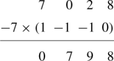
(1−1−1001−230004138)

Here the calculation was Row 3 – (7) × (Row 2), and the calculation was as follows:

Stage 3
Divide the third equation by the coefficient of z:
(1−1−1001−2300012441)
Back-substitution: We have now finished the elimination stage and we can easily solve the equations using back substitution.
From the third equation, I3=2441![]() . Find I2 from the second equation:
. Find I2 from the second equation:
I2−23I3=0 I2−23×2441=0?????⇔?????I2=1641.

Substitute into the first equation to find I1:
I1-1641-2441=0????⇔?????I1=4041
![]()
So the solution of the system of equations is (4041,?1641,?2441).
Check: To check, substitute I1=4041,?I2=1641,?and?I3=2441![]() into the original equations
into the original equations
I1−I2−I3=03I2−2I3=07I1+2I3=8

giving
4041−1641−2441?=?0,?which?is?true3(1641)−2(2441)?=?0,?which?is?true7(4041)+2(2441)?=?8,?which?is?true.
Indeterminacy and inconsistency
When we analysed systems of equations in Section 13.5, we saw that one of the equations reducing to 0 =0, indicates that we have an indeterminate system; that is that there will be many solutions. If, in the process of performing Gauss elimination, we find a row of zeros then we know that we have an indeterminate system. We can use the remaining equations to eliminate as many of the unknowns as possible, giving a solution which will still involve one or more of the variables. This will give a whole line or possibly (in three dimensions) a plane of solutions.
If we come across a row that is zero everywhere in the matrix of coefficients but has a non-zero constant term we have found an equation 0 = c, which is false. This is an inconsistent system and has no solutions.
Order of the equations
At the beginning of each stage in Gauss elimination, the order of the rows may be swapped (other than those already used in previous stages as the pivotal equation). We will have to swap the equations if the next ‘pivotal’ equation has a zero coefficient for the next variable to be eliminated. It is usual, although we have not illustrated this point, to always consider swapping the order of the equations, in order to choose the equation with the largest absolute value of the coefficient in the term to be used for eliminating, as the pivotal equation. This is called partial pivoting. This procedure as an attempt to avoid problems with equations that may become ill conditioned in the course if performing the elimination. The equations are ill conditioned when a small change in the coefficients of the equations causes a large change in the values of the solutions, and in such equations rounding errors can become large and cause significant inaccuracies in the solutions. We have not performed partial pivoting in these examples as they are only presented to give an idea of the method. It is assumed that for any real life problem a computer algorithm will be used to solve the system of equations, and such an algorithm will incorporate partial pivoting.
13.6 The inverse and determinant of a 3 × 3 matrix
Finding the inverse by elimination
To find the inverse using elimination, we write the matrix we need to invert on the left and the unit matrix on the right. We perform operations on both matrices at the same time. The method, called Gauss–Jordan elimination, begins in the same way as Gauss elimination. When we have upper triangular form for the matrix we metaphorically turn the problem upside down and eliminate the upper triangle also.
Example 13.28
Find the inverse of
(40−4342−1−11).

Solution We start by writing the matrix along with the unit matrix
(40−4100342010−1−11001).
Stage 1
Step 1: Divide the first row by a11
(10−10.2500342010−1−11001).

Step 2: Eliminate the first column below a11 by subtracting multiples of the first row from the second and third rows
(10−10.2500045−0.75100−100.2501).

The calculations were as follows:
Row 2–3 × Row 1
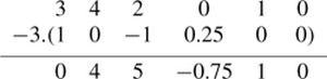
Row 3 – (−1) × Row 1
Stage 2
Step 1: Divide the second row by a22(4)
(10−10.2500011.25−0.18750.2500−100.2501).
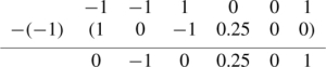
Step 2: Eliminate the elements in the second column below a22 by subtracting multiples of the second row from the third row
(10−10.2500011.25−0.18750.250001.250.06250.251).

The calculations were as follows:
Row 3 – (−1) × Row 2

Stage 3
Step 1: Divide the third row by a33 (1.25):
(10−10.2500011.25−0.18750.2500010.050.20.08)
Step 2: Turn the problem metaphorically upside down and use the third row to eliminate elements in the third column above a33 by subtracting multiples of the third row from the first row and the second row
(1000.30.20.8010−0.250−10010.050.20.8)

The calculations were as follows:
Row 1 – (−1) × Row 3

Row 2 – 1.25 × Row 3

The matrix on the right-hand side is now the inverse of the original matrix.
The inverse is
(0.30.20.8−0.250−10.050.20.8)
Check: Multiply the original matrix by its inverse
(40−4342−1−11)(0.30.20.8−0.250−10.050.20.8)????????=(4(0.3)+0(−0.25)−4(0.05)4(0.2)+0(0)−4(0.2)4(0.8)+0(−1)−4(0.8)3(0.3)+4(0.25)+2(0.05)3(0.2)+4(0)+2(0.2)3(0.8)+4(−1)+2(0.8)−1(0.3)−1(−0.25)+1(0.05)−1(0.2)−1(0)+1(0.2)−1(0.8)−1(−1)+1(0.8))????????=(100010001)

Therefore we have correctly found the inverse of the matrix.
The determinant of a 3 × 3 matrix
The definition of the (2 × 2) determinant has been given as
|a1b1a2b2|=a1b2−a2b1.

Each of the terms on the right-hand side of this definition is of the form ai, bj where i and j are different choices of the numbers 1 and 2. We can define higher order determinants by using ideas of permutations. We notice that the term a1b2 above has a positive sign because the indices 1 and 2 appear in order, whereas the term a2b1 has a negative sign because the indices 2,1 are reversed.
To define
|a1b1c1a2b2c2a3b3c3|
we write down all terms of the form ai b jck and give each term a + sign or a – sign depending on whether the permutation ijk is even or odd. A permutation of 123 is even if it can be achieved by an even number of swaps of the numbers, beginning with the order 123. If it can only be obtained by an odd number of swaps then the permutation is odd. For example, 231 is even because we can reach it by first swapping 1 and 2 giving 213 and then swapping 1 and 3. Alternatively, we could have interchanged 2 and 3 giving 132 and 1 and 3 giving 312, 2 and 1 giving 321,3 and 2 giving 231. Whatever way we use to get to the order 231 involves an even number of steps. Similarly we say that a permutation of 123 is odd if it involves an odd number of adjacent interchanges.
This definition gives the determinant of a 3 × 3 array as
|a1b1c1a2b2c2a3b3c3|=a1b2c3−a1b3c2−a2b1c3+a2b3c1+a3b1c2−a3b2c1
This expression may be written in such a way that it involves 2 × 2 determinants as follows:
a1b2c3−a1b3c2−a2b1c3+a3b1c2+a2b3c1−a3b2c1????????=a1(b2c3−b3c2)−b1(a2c3−a3c1)+c1(a2b3−a3b2)????????=a1|b2c2b3c3|−b1|a2c2a3c3|+c1|a2b2a3b3|.
The 2 × 2 determinants that appear in this expression are called minors. This formula for the determinant is called the expansion by the first row, because the numbers a1, b1, c1 which multiply the minors are from the first row of the matrix.
Note that the minor multiplying a1 is the (2 × 2) determinant obtained from the original array by crossing out the row and column in which al appears, as follows
gives the minor of a1as
|b2c2b3c3|.

Similarly, the number multiplying b1 is the determinant found by crossing out the row and the column in which b1 appears.
We could also find the determinant by expanding about the first column
a1b2c3−a1b3c2−a2b1c3+a2b3c1+a3b1c2−a3b2c1????????=a1(b2c3−b3c2)−a2(b1c3−b3c1)+a3(b1c2−b2c1)????????=a1|b2c2b3c3|−a2|b1c1b3c3|+a3|b1c1b2c2|.
Again we see that the minor of a2, for instance, can be found by crossing out the row and column that a2appears in from the original array.
To find the sign multiplying each term in the expansion for the determinant we can remember the following pattern
+−+−+−+−+

To find the determinant we can expand about any row and column, multiplying each term aijby its respective minor and find the sign by multiplying by (−l)i+j.
Example 13.29
Find the following determinant
|−1236−1240−1|
Solution Expanding about the first row
|−1236−1240−1|=−1|−120−1|−2|624−1|+3|6−140| =−1(1−0)−2(−6−8)+3(0+4)=−1+28+12=39.

Alternatively, expanding about the first column we get
−1|−120−1|−6|230−1|+4|23−12|=−1(1−0)−6(−2−0)+4(4−(−3))=−1+12+28=39.

The inverse of a matrix using (Adjoint(A))/|A|
We have already seen how to find the inverse of a matrix by using elimination. It is also possible to find the inverse by the following procedure:
(1) Find the matrix of minors.
(2) Multiply the minor for row i and column j by (−l)i+j. This is then called the matrix of cofactors.
(3) Take the transpose of the matrix of cofactors to find the adjoint matrix.
(4) Divide by the determinant of the original matrix.
This procedure rarely needs to be used and only usually if we have a matrix which involves some unknown variables or expresses some formula and we would like to find the inverse formula. It would never be used as a numerical procedure, as it is both numerically unstable and also uses a very large number of operations (of the order of n! operations, where n is the dimension of the matrix, whereas elimination is only of the order of n3).
Example 13.30
Find the inverse of
(40−4342−1−11)

using A−1 =(Adjoint(A))/|A|.
Solution Find the matrix of minors for each term in the matrix. The minor for the ith row and jth column is found by crossing out that row and column and finding the determinant of the remaining elements.
This gives the matrix of minors as
(|42−11||32−11||34−1−1||0−4−11||4−4−11||40−1−1||0−442||4−432||4034|)=(651−40−4162016).
To find the matrix of cofactors we multiply by the pattern
+−+−+−+−+

giving
(6−5140416−2016).

To find the adjoint, we take the transpose of the above, giving
(6416−50−201416).
Now we find the determinant – expanding about the first row, this gives
4(4−(−2))−0(3(1)−2(−1))−4(3(−1)−(−1)(4))=20
![]()
Finally, we divide the adjoint by the determinant to find the inverse giving
120(6416−50−201416)=(0.30.20.8−0.250−10.050.20.8).

Check: To check that the calculation is correct, we multiply the original matrix by the inverse. If we get the unit matrix as the result we can conclude that we have indeed found the inverse.
(40−4342−1−11)(0.30.20.8−0.250−10.050.20.8)=(100010001)

which is correct.
13.7 Eigenvectors and eigenvalues
In Example 13.17, we looked at the problem of scaling along the line x =y and we saw that the matrix
(32121232)
represents a scaling along the line y = x and it leaves points along the line y = –x unchanged. This means that any vector in the direction (1,1) will simply be multiplied by 2 and any vector in the direction (–1,1) will remain unchanged after multiplication by this matrix. Other vectors will undergo a mixed effect.
Supposing we know that a matrix A represents a scaling but without knowing the direction of the scaling or by how much it scales. Is there any way we can find that direction and the scaling constant?
The problem then is to find a vector v which is simply scaled by some currently unknown amount λ when multiplied by A, and v must be such that
Av?=?λv
![]()
If we manage to find values of λ and v we call these the eigenvalues and eigenvectors of the matrix A.
We shall solve this for
(32121232)

as we know the result that we expect to get.
Example 13.31
Find λ and v such that Av = λ v where
A?=?(32121232).
Solution Subtract λv from both sides of the equation
Av?=λv???????⇔????????Av−λv=0?????????(32121232)v−λv=0
We put in the unit matrix as v = Iv and combine the terms.
(32121232)v−λ(1001)v=(00)???????????(32−λ121232−λ)v=(00).
Now substitute
v=(xy)

giving
(32−λ)x+12y=012x+(32−λ)y=0.
Unfortunately, the solution to this gives x = 0 and y = 0, which is not very enlightening (it is called the trivial solution).
However, we started by saying that we wanted to find the direction in which this matrix scaled any vector. That is, we want to find a whole line of solutions. We can use a result that we found from solving systems of equations. The equations may have a whole line of solutions if the determinant of the coefficients is 0.
Hence, we need to find λ such that
|32−λ121232−λ|=0.

Expanding the determinant gives
(32−λ)(32−λ)−14=094−3λ+λ2−14=0⇔λ2−3λ+2=0.
This factorizes to
(λ−2)(λ−1)=0????⇔????λ=1∨λ=1.
![]()
Hence, the eigenvalues of the matrix A are 1 and 2. To find the vectors which go with each of these eigenvalues we substitute into the equations
(32−λ)x+12y=012x+(32−λ)y=0.

For λ = 2
−12x+12y=012x−12y=0.
We notice that these equations are dependent, which we would have expected as by setting the determinant = 0 we were looking for an undetermined system.
We have
−12x+12y?=0??????⇔??????x=y.
![]()
This means that any vector (x, y) where y = x will be scaled by 2 if multiplied by the matrix A. The eigenvector can be given as (1,1) as it is only necessary to indicate the direction.
The other eigenvalue, λ = 1, gives
12x+12y?=012x+12y?=0.

Again, the equations are dependent and we have x + y = 0. The eigenvector is any vector (x, y) where x = –y so this gives the direction (–1,1).
As not all matrices represent scaling, it is not always possible to find real eigenvalues. In particular, a rotation matrix has no real eigenvalues for angle of rotation, θ ≠ 0. Another point to note is that in this example the eigenvectors were at right angles to each other. This is only true for symmetric matrices (which we had in this case).
The method can be summarized as follows: To find the eigenvalues and eigenvectors of A
(1) Solve |A – λI| = 0 to find the eigenvalues. This is called the characteristic equation.
(2) For each value of λ found, substitute into (A – λI)v = 0 and find v. This will be an undetermined system so we shall find at least a whole line of solutions. Choose any vector lying in the direction of the line.
Example 13.32
Find the eigenvectors and eigenvalues of
(132−4).

Solution Solve |A – λI| = 0, which gives
|1?−λ32−4−λ|=0⇔(1−λ)(−4−λ)−6=0⇔λ2+3λ−10=0⇔(λ+5)(λ−2)=0⇔λ=−5?or?λ=2.
For each value of λ solve
(1?−λ32−4−λ)(xy)=(00).

For λ = −5, this gives
(6321)(xy)=(00)??????????⇒??????????6x+3y=02x+y=0
We see that these equations are dependent. Solving the first one
6x+3y=0⇔??????2x+y=0y=−2x

The vector is therefore (x, y) where y = −2x, giving (x, −2x). We only need the direction of the vector so choose (1, −2) by substituting x = 1
For λ = 2 we get
(−132−6)(xy)=(00)?⇒−x+3y=02x−6y=0

Solving
−x+3y=0?????⇔?????x=3y
![]()
Hence, we have (x, y) where x =3 y giving (3 y, y). Substitute y = 1 giving the vector as (3,1).
We have shown that the matrix
(132−4)

has eigenvalue −5 with eigenvector (1, −2) and eigenvalue 2 with eigenvector (3,1).
13.8 Least squares data fitting
Matrix methods can be employed to the problem of finding the ‘best fit’ line through a set of data. In Chapter 2 we performed a fit by eye to a set of data points. We drew a scatter diagram of the data and if the data appeared, more or less, to fit on a line then we would draw the line by hand and then use any two points lying on the line, to find the equation of the line. We do not expect experimental data to be exact and that is the reason that the data points do not lie exactly on a line. We shall now look at the method of least squares, which can be used to compute the ‘best fit’ line. The method is called ‘least squares’ because it minimizes the squared error between the data points and the equation of the line found. The method is justified in the following example.
We start with two sets of data which we suspect are related linearly.
Example 13.33
A student was late for a particularly interesting engineering maths lecture and was therefore walking briskly toward the lecture hall in a straight line at approximately constant speed b. The student's position x (metres) at time t (seconds) is given by

We can plot these points on a scatter diagram, as in Figure 13.18.

We can see that they lie on an approximate straight line. We need to decide which is the ‘best’ straight line to draw. One way is to fit the straight line, y = a + bx, to a set of data points (xi, yi) so that the sum of the squares of the vertical distances of the points from the straight line drawn is minimum. This is illustrated in Figure 13.19.
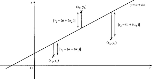
In order to fit the line y = a +bx, we can vary the values of a and b until it satisfies our condition for minimum squared error. If the data points are (xi, yi), then the sum of the squares of the errors is given by
E?=?∑i(yi−a−bxi)2
![]()
We can vary a and b to make this a minimum. However, E is a function of two variables a and b. We know how to find the minima or maxima with respect to one variable, which we looked at in Chapter 11. We shall look in more detail at functions of two variables in Chapter 17. To minimize with respect to two variables we begin by differentiating with respect to each variable in turn keeping the other variable constant. This is called partial differentiation. The ideas used in finding stationary values are the same as that for one variable although the method of distinguishing between types of stationary values is slightly more involved because the function represents a two-dimensional surface drawn in three dimensions rather than a simple curve. A partial derivative is indicated by using a curly d, ∂, for the derivative and ∂ E/∂a is read as ‘partial dE by da’
∂E∂a?=?−2∑i(yi−a−bxi)∂E∂b?=?−2∑ixi(ti−a−bxi)

For a minimum value we must have ∂E/∂a = 0 and ∂E/∂b = 0 giving
−2∑i(yi−a−bxi)=0⇔∑iyi−∑ia−b∑ixi=0−2∑ixi(yi−a−bxi)=0⇔∑ixiyi−a∑ixi−b∑ix2i=0
Finally, we get the normal equations
an+b∑ixi=∑iyia∑ixi+b∑ix2i=∑ixiyi
where n is the number of data points.
Here, we have not attempted to justify that this is actually a minimum point (we have only shown it to give a stationary point). We can now illustrate the method for finding the values of a and b which minimize the sum of the squared errors. At the start of this example we had a set of data which we wish to fit to a function x = a+bt where the dependent variable is x and the independent variable is t. We wish to find the values of a and b so that x = a + bt gives a least squares fit to the data. The number of data points is 6, so we have as the normal equations:
6a+b6Σi=1ti=6Σi=1xia6Σi=1ti+b6Σi=1t2i=6Σi=1tixi
Make a table from the data, as in Table 13.1.
Table 13.1
A table made from the data of Example 13.32
| t | x | t2 | tx |
| 0 | 100 | 0 | 0 |
| 5 | 111 | 25 | 555 |
| 10 | 119 | 100 | 1190 |
| 15 | 132 | 225 | 1980 |
| 20 | 151 | 625 | 3775 |
| 75 | 753 | 1375 | 10 300 |

Then the normal equations become:
6a+75b=75375a+1375b=10300

Solving
450a+5625b=56475450a+8250b=618002625b=5325
⇒b≈2.036a+75(2.03)=754⇒a≈100.14
We have a = 100.14 and b = 2.03. Hence, the line of best fit is
x=100.14+2.03t.
![]()
Curve fitting
The same method for fitting a straight line can be generalized to fit any polynomial. For example, it could appear that our data would be better fitted to a parabola.
y=b0+b1x+b2x2
![]()
The normal equations in this case are
b0n+b1∑ixi+b2∑ix2i=∑iyib0∑ixi+b1∑ix2i+b2∑ix3i=∑ixiyib0∑ix2i+b1∑ix3i+b2∑ix4i=∑ix2iyi

We can solve these system of equations using Gaussian elimination.
Example 13.34
Find the best fit parabola by the method of least squares for (0,3) (1,1) (2,0) (4,1) (6,4).
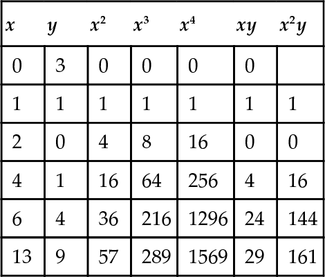
Solution The data are given in Table 13.2. The normal equations are:
5b0+13b1+57b2=913b0+57b1+289b2=2957b0+289b1+1569b2=161

Table 13.2
Table made from the data of Example 13.34
| x | y | x2 | x3 | x4 | xy | x2y |
| 0 | 3 | 0 | 0 | 0 | 0 | |
| 1 | 1 | 1 | 1 | 1 | 1 | 1 |
| 2 | 0 | 4 | 8 | 16 | 0 | 0 |
| 4 | 1 | 16 | 64 | 256 | 4 | 16 |
| 6 | 4 | 36 | 216 | 1296 | 24 | 144 |
| 13 | 9 | 57 | 289 | 1569 | 29 | 161 |
Solving these using Gauss elimination gives
(513579135728929572891569161)
Stage 1
(12.611.41.8135728929572891569161)
(12.611.41.8023.2140.85.60140.8919.258.4)
Stage 2
(12.611.41.8016.0690.2410140.8919.258.4)(12.611.41.8016.0690.2410064.68524.467)
Stage 3
(12.611.41.8016.0690.2410010.378)Back−substitutionb0+2.6b1+11.4b2=1.8b1+6.069b2=0.241b2=0.378

gives b2 = 0.378, b1 = −2.054, and b0= 2.831.
Hence, the best fit parabola is y = 2.831 – 2.054x + 0.378x2.
13.9 Summary
1. Matrices are used to represent information in a way suitable for use by a computer. They can represent, among other things, systems of linear equations, transformations, and networks. A matrix is a rectangular array of numbers of dimension m × n where m is the number of rows and n is the number of columns.
2. To add or subtract matrices add or subtract each corresponding element. The matrices must be of exactly the same dimension. To multiply two matrices, C = AB, the number of columns in matrix A must equal the number of rows in matrix B. The i, jth element of C is found by multiplying the ith row of A by the jth column of B.
3. The unit matrix, I, leaves any matrix unchanged under multiplication.
I=?(1010)(2?dimensions)I=?(100010001)(3?dimensions)

IA = AI = A where A is any matrix.
4. The inverse of a matrix is represented by A−1 and can be found for square, non-singular matrices. A matrix is singular if its determinant is 0.
5. The 2 × 2 determinant is defined by
|abcd|=ad−cb.
6. The inverse of a 2 × 2 non-singular matrix (abcd) is
is
1(ad−cb)(d−b−ca).

7. Transformations of the plane ![]() 2 can be defined using vectors and matrices as in Section 13.13.
2 can be defined using vectors and matrices as in Section 13.13.
8. Systems of linear equations may be determined (a single solution), indeterminate (many solutions) or inconsistent (no solutions).
9. Systems of linear equations can be solved using Gaussian elimination.
10. The inverse of a matrix, if it exists, can be found using Gauss–Jordan elimination.
11. The determinant of a 3 × 3 matrix may be found by expanding about any row or column, where
|a1b1c1a2b2c2a3b3c3|=a1|b2c2b3c3|−b1|a2c2a3c3|+c1|a2b2a3b3|
gives the expansion about the first row.
12. The inverse of a non-singular matrix can be found using
A−1=(1/|A|)(Adjoint(A)).
![]()
13. The eigenvalues and eigenvectors of a matrix A are the values of and v such that Av = λv.
14. The method of least squares is used to fit a line or a curve through experimental data in such a way as the sum of the square of the errors is a minimum.
13.10 Exercises
A=(230−402)???????B=(2−10161034)C=(4??0??−1)???????D=(03−14)E=?(32−1−23)
Find the following, where possible
(b) ATB
(c) AB
(d) BA
(e) CT
(f) AC
(g) CA
(h) CB
(i) 3CA
(j) D+E
(k) 3D−12![]() E
E
(l) 12![]() B+A
B+A
(m) B2
(n) E3
(o) AC2
A=(a11a12a21a22)??B=(b11b12b21b22)??C=(c11c12c21c22)
to justify the associative law for 2 × 2 matrices
A(BC)?=?(AB)C
![]()
13.3. Find a real square matrix which is both symmetric and skew symmetric.
13.4. A network as in Figure 13.20(a), (b), or (c) can be used to represent an electrical network, as system of one-way streets, or a communication system. An incidence matrix can be defined for a network in the following way (the lines are called arcs and the dots are called vertices).
aij = 1 if the arc j is leaving the vertex i
aij =–1 if the arc j is entering the vertex i
aij = 0 if the arc j does not touch the vertex i
For instance, Figure 13.20(a) has incidence matrix
Vertex?????123?????(a-110?Arcb0-11?c-101)

(i) Find incidence matrices for the networks in Figure 13.20(b) and (c).
(b) Draw networks that have the following incidence matrices
(i)
Vertex Arcabc1234(-1110-1010-1000)

(ii)
Vertex Arcabcde123(-10-1101-10-110110-1)


13.5. Represent the following transformations using matrices and vectors. In each case, apply the transformations to A(0,0), B(1,0), C(1,1), and D(0,1) to find their images A′, B′, C′ and D′ and draw your result:
(a) Rotation about the origin through 120º.
(b) Translation by (–4, 1).
(c) Reflection in the x-axis.
(d) Scaling in the y-direction by 5.
(e) Rotation through 120º about the origin followed by a translation by (–2,3).
(f) Translation by (–1,3) followed by rotation through 120º about the origin.
(g) Rotation through 120º about the origin followed by scaling by 5 in the y-direction.
(h) Reflection in the line y = x.
(i) Scaling along a line at a 30º angle to the x-axis, by a factor of 4.
(k) Find inverse transformations for those given in parts (a),(b),(c),(e),(g), and (i) and check in each case that the inverse transformation returns A′, B′, C′, and D′ to A,B,C,D.
13.6. Sketch the following systems of equations and solve them using Gauss elimination. In each case, state whether the system is determined, indeterminate, or inconsistent.
(b) x+y=3x-y=7![]()
(c) 3x+2y=1-2x-43y=0
(d) -5x-y=510x+2y=-10![]()
(e) 3x+2y=-1710x+y=0![]()
(f) x+6y=43x+18y=10![]()
(g) -3x+2y=11.5x-y=0.5![]()
(h) -7x+8y=-10-2x+y=-8.![]()
13.7. Solve the following using Gauss elimination. In each case state whether the system is determined, indeterminate or inconsistent.
(a) 2x-3y-z=45x+5y+2z=-23 x ???+????z=-1
(b) 4x-y-2z=403x+y+9z=5 x-y+z=-55
(c) x+y-3z =8-10x+6y ????=-14??12x-4y-6z=30
(d) ?x-y+z=3x+z =3-4x-y-4z=-10.
13.8. Find inverses of the following matrices A, if they exist, and check that A−1A = I
(b) (23-16)![]()
(c) (2-110-5)![]()
(d) (1-10-242-312)
(e) (051-153202)
(f) (1-12613-5-2-1)
13.9. Find the following determinants:
(b) |51-62|
(c) |3-21010321|
(d) |6-3-21-180-10|.
13.10. The vector product of two three-dimensional vectors can be defined using a determinant as follows:
(a1,?a2,?a3)×(b1,b2,b3)=|ijka1a2a3b1b2b3|

where i, j, and k are the unit vectors in the x, y, and z directions, respectively. Use this definition to find the following:
(b) (12,12![]() , −1) × (0,0,3).
, −1) × (0,0,3).
13.11. The scalar triple produce of three vectors a, b, c, given by a. (b × c) can be found using a determinant as follows:
(a1,?a2,?a3)⋅((b1,b2,b3)×(c1,?c2,?c3))???????=|a1a2a3b1b2b3c1c2c3|

The absolute value of this can be interpreted as the volume of the parallelepiped which has a, b, c as its adjacent edges.
(a) Find the volume of the parallelepiped with adjacent edges given by the vectors
(i) (1,0, −3), (0,1,1), and (3,0,1)
(ii) (1, −2,2), (3,2, −1), and (2, 1, 1)
(b) Explain why in case (a), (ii) you could conclude that the three vectors lie in the same plane.
13.12 In a homogeneous, isotropic and linearly elastic material it is found that the strains on a section of the material, represented by εx, εy, and εz for the x-, y-, and z-directions, respectively, can be related to the stresses, (σx, σy, and σzby the following matrix equation.
(ɛxɛyɛz)=1E(1−ν−ν−ν1−ν−ν−ν1)(σxσyσz)
where E is the modulus of elasticity (also called Young's modulus) and v is Poisson's ratio which relates the lateral and axial strains. Find (σx, σy, σz, in terms of εx, εy, and εzand express the relationship in matrix form.
13.13. Find eigenvalues and eigenvectors of the following:
(6−102)

(b)
(151−3)

(c)
(3212).

13.14. A simple circuit comprising a variable voltage Vs, a diode and a resistor is shown in Figure 13.21. As Vs is varied, values of VR and I are recorded. The values are given in Table 13.3.
Using the method of least squares, determine Z and VD in the equation VR = ZI + VD.

13.5 In an attempt to measure the stiffness of a spring the length of the spring under different loads was measured and the data is given in Table 13.4
(a) Use the data to find an equation that could be used to find the length of the spring given the weight.
(b) From your equation estimate, if possible, the length of the spring when
(ii) the load is 5 kg.
Table 13.4
Loads against spring length for Problem 13.15
| Load (kg) | Length (cm) |
| 0 | 10 |
| 0.5 | 10.8 |
| 1 | 11.5 |
| 2 | 14 |
| 3 | 15.5 |
| 4 | 17.5 |
13.16. The power dissipation of a n–p–n silicon transistor is thought to vary linearly with temperature. The data given in Table 13.5 were recorded experimentally
Plot these points on a scatter diagram and use the method of least squares to obtain a and b in the equation relating the power (P) to the temperature (T); P= a +bT.
Table 13.5
Power dissipation of a n–p–n silicon transistor recorded against temperature
| Temperature (°C) | Power dissipation (W) |
| 25 | 10 |
| 60 | 7.9 |
| 100 | 5.7 |
| 120 | 4.8 |
| 140 | 3.5 |
13.17. Fit parabolas to the following sets of data:
(a) (–1,0), (0, −1), (1,4), (2, 14) (3,32)
(b) (–1, 5.5), (0, 1.5), (0.5, 0.5), (2, 5).