14.6 Solving systems of differential equations

Search in book...
Toggle Font Controls
Create new playlist

Name your new playlist

Playlist description (optional)
Sign In

Email address

Password

Forgot Password?

or

Continue with Facebook

Continue with Google
Sign Up

Full Name

Email address

Confirm Email Address

Password

or

Continue with Facebook

Continue with Google

14.6 Solving systems of differential equations

To solve a system of differential equations we can combine the equations into a single differential equation using substitution. In this case we can use the method as outlined in Section 14.5. Alternatively, we can solve the system directly using matrices.

We follow the same pattern as in Section 14.4 for first-order systems. We solve the homogeneous equation, to find the complementary function and then find a particular solution. The sum of these two terms gives a general solution to the system.

Example 14.10

Find the displacement of the spring after time t described by the system of differential equations

$\frac{d}{d t} (\begin{array}{l} x_{1} \\ x_{2} \end{array}) = (\begin{array}{l} 0 & 1 \\ - k / m & - r / m \end{array}) ? (\begin{array}{l} x_{1} \\ x_{2} \end{array}) ? (\begin{array}{l} 0 \\ 1 / m \end{array}) ? f (t)$ $\frac{d}{d t} (\begin{array}{l} x_{1} \\ x_{2} \end{array}) = (\begin{array}{l} 0 & 1 \\ - k / m & - r / m \end{array}) ? (\begin{array}{l} x_{1} \\ x_{2} \end{array}) ? (\begin{array}{l} 0 \\ 1 / m \end{array}) ? f (t)$

si194_e

in the case where the mass on the spring is 1, the damping constant r = 5, the spring constant k = 4, the forcing function f(t) = t, and the initial extension of the spring is 0 with 0 initial velocity.

Solution Substituting the given values for m, r, k, and f, we have the system

$\frac{d}{d t} (\begin{array}{l} x_{1} \\ x_{2} \end{array}) = (\begin{array}{l} 0 & 1 \\ - 4 & - 5 \end{array}) ? (\begin{array}{l} x_{1} \\ x_{2} \end{array}) + (\begin{array}{l} 0 \\ 1 \end{array}) ? f (t) .$ $\frac{d}{d t} (\begin{array}{l} x_{1} \\ x_{2} \end{array}) = (\begin{array}{l} 0 & 1 \\ - 4 & - 5 \end{array}) ? (\begin{array}{l} x_{1} \\ x_{2} \end{array}) + (\begin{array}{l} 0 \\ 1 \end{array}) ? f (t) .$

si195_e

Step 1

Solve the homogeneous system with f(t) = 0, giving

$\frac{dx}{d t} = Ax ? where ? A = (\begin{array}{l} 0 & 1 \\ - 4 & - 5 \end{array}) .$ $\frac{dx}{d t} = Ax ? where ? A = (\begin{array}{l} 0 & 1 \\ - 4 & - 5 \end{array}) .$

si196_e

Try solutions of the form x = v e^λt, where v is a constant vector. Then dx/dt = λv e^λt. Substitute for x and dx/dt dt into dx/dt = Ax, giving

$λ ? v ? e^{λ t} = A ? v ? e^{λ t}$ $λ ? v ? e^{λ t} = A ? v ? e^{λ t}$

as e^λt≠ 0, we have

$\begin{array}{l} λ ? v = A ? v \\ Av = λ ? v \end{array}$ $\begin{array}{l} λ ? v = A ? v \\ Av = λ ? v \end{array}$

si198_e

which we recognize as the eigenvalue problem of Chapter 13. In this case, however, we shall allow the possibility of complex eigenvalues.

The solutions for λ are found by solving |A – λI| = 0 as

$A = (\begin{array}{l} 0 & 1 \\ - 4 & - 5 \end{array})$ $A = (\begin{array}{l} 0 & 1 \\ - 4 & - 5 \end{array})$

si199_e

this gives

$\begin{array}{l} | \begin{array}{l} - λ \\ - 4 \end{array} & \begin{array}{l} 1 \\ - 5 - λ \end{array} | = 0 \\ \Leftrightarrow & λ (5 + λ) + 4 = 0 \\ \Leftrightarrow & λ^{2} + 5 λ + 4 = 0 \\ \Leftrightarrow & λ = \frac{- 5 \pm \sqrt{25 - 16}}{2} \\ \Leftrightarrow & λ = \frac{- 5 \pm 3}{2} \Leftrightarrow λ = - 4 ? \lor ? λ = - 1. \end{array}$ $\begin{array}{l} | \begin{array}{l} - λ \\ - 4 \end{array} & \begin{array}{l} 1 \\ - 5 - λ \end{array} | = 0 \\ \Leftrightarrow & λ (5 + λ) + 4 = 0 \\ \Leftrightarrow & λ^{2} + 5 λ + 4 = 0 \\ \Leftrightarrow & λ = \frac{- 5 \pm \sqrt{25 - 16}}{2} \\ \Leftrightarrow & λ = \frac{- 5 \pm 3}{2} \Leftrightarrow λ = - 4 ? \lor ? λ = - 1. \end{array}$

si200_e

Now, we find the eigenvector v to go with each eigenvalue by solving $(A - λ I) v = 0.$ $(A - λ I) v = 0.$

$(\begin{array}{l} - λ & 1 \\ - 4 & - 5 - λ \end{array}) ? (\begin{array}{l} ν_{1} \\ ν_{2} \end{array}) = (\begin{array}{l} 0 \\ 0 \end{array}) .$ $(\begin{array}{l} - λ & 1 \\ - 4 & - 5 - λ \end{array}) ? (\begin{array}{l} ν_{1} \\ ν_{2} \end{array}) = (\begin{array}{l} 0 \\ 0 \end{array}) .$

For λ = − 4

$(\begin{array}{l} 4 & 1 \\ - 4 & - 1 \end{array}) ? (\begin{array}{l} ν_{1} \\ ν_{2} \end{array}) = (\begin{array}{l} 0 \\ 0 \end{array}) .$ $(\begin{array}{l} 4 & 1 \\ - 4 & - 1 \end{array}) ? (\begin{array}{l} ν_{1} \\ ν_{2} \end{array}) = (\begin{array}{l} 0 \\ 0 \end{array}) .$

si203_e

Multiplying out, this gives

$\begin{array}{l} 4 ? ν_{1} + ν_{2} = 0 \\ - 4 ? ν_{1} - ν_{2} = 0. \end{array}$ $\begin{array}{l} 4 ? ν_{1} + ν_{2} = 0 \\ - 4 ? ν_{1} - ν_{2} = 0. \end{array}$

si204_e

These equations are dependent, solving either one of them we find

$\begin{array}{l} 4 ? ν_{1} = - ν_{2} \\ ν_{2} = - 4 ν_{1} . \end{array}$ $\begin{array}{l} 4 ? ν_{1} = - ν_{2} \\ ν_{2} = - 4 ν_{1} . \end{array}$

si205_e

The vector is given by (v₁, −4v₁). As we are interested only in the direction of the vector we can set v₁ = 1 giving the eigenvector as (1, −4).

For A = −1 we get

$(\begin{array}{l} 4 & 1 \\ - 4 & -1 \end{array}) ? (\begin{array}{l} ν_{1} \\ ν_{2} \end{array}) = (\begin{array}{l} 0 \\ 0 \end{array}) .$ $(\begin{array}{l} 4 & 1 \\ - 4 & -1 \end{array}) ? (\begin{array}{l} ν_{1} \\ ν_{2} \end{array}) = (\begin{array}{l} 0 \\ 0 \end{array}) .$

si206_e

Multiplying out we get

$\begin{array}{l} ν_{1} + ν_{2} = 0 \\ - 4 ν_{1} - 4 ν_{2} = 0. \end{array}$ $\begin{array}{l} ν_{1} + ν_{2} = 0 \\ - 4 ν_{1} - 4 ν_{2} = 0. \end{array}$

si207_e

These equations are dependent, solving either one we get

$ν_{2} = - ν_{1} .$ $ν_{2} = - ν_{1} .$

The vector is given by (v₁, – v₁). As we are interested only in the direction of the vector we can set v₁ = 1 giving the eigenvector as (1, −1).

Therefore, we have the complementary function for x as

$x ? = a (\begin{array}{l} 1 \\ - 4 \end{array}) e^{- 4 t} + b (\begin{array}{l} 1 \\ - 1 \end{array}) e^{- t}$ $x ? = a (\begin{array}{l} 1 \\ - 4 \end{array}) e^{- 4 t} + b (\begin{array}{l} 1 \\ - 1 \end{array}) e^{- t}$

si209_e

where a and b are arbitary constant scalars.

Step 2

Find a particular solution to the equation dx/dt = Ax + bt. For this equation, the forcing function is bt so we try a particular solution of the form x = c₁t + c ₀ where c₀ and c₁ are constant vectors. We see that this is similar to the choice of trial solution suggested in Table 14.1 but the constant terms are now constant vectors.

$\begin{array}{l} x = c_{1} t + c_{0} \\ \Rightarrow ? ? ? ? ? ? ? ? d x / d t = c_{1} . \end{array}$ $\begin{array}{l} x = c_{1} t + c_{0} \\ \Rightarrow ? ? ? ? ? ? ? ? d x / d t = c_{1} . \end{array}$

si210_e

Substitute this trial solution into

$dx / d t = Ax + b t$ $dx / d t = Ax + b t$

giving

$c_{1} = A (c_{1} t + c_{0}) + b t .$ $c_{1} = A (c_{1} t + c_{0}) + b t .$

We can equate vector coefficients of t and the constant terms on both sides giving

$\begin{matrix} 0 = {Ac}_{1} + ? b \\ c_{1} = {Ac}_{0} . \end{matrix}$ $\begin{matrix} 0 = {Ac}_{1} + ? b \\ c_{1} = {Ac}_{0} . \end{matrix}$

si213_e

We solve these two matrix equations

$\begin{matrix} 0 = {Ac}_{1} + ? b \\ \Leftrightarrow {Ac}_{1} = - b . \end{matrix}$ $\begin{matrix} 0 = {Ac}_{1} + ? b \\ \Leftrightarrow {Ac}_{1} = - b . \end{matrix}$

si214_e

Pre-multiply by A⁻¹ (if it exists) giving

$c_{1} = - A^{−1} b$ $c_{1} = - A^{−1} b$

$A ? = (\begin{array}{l} 0 & 1 \\ - 4 & - 5 \end{array})$ $A ? = (\begin{array}{l} 0 & 1 \\ - 4 & - 5 \end{array})$

si216_e

we have

$A^{−1} = \frac{1}{4} (\begin{array}{l} - 5 & - 1 \\ 4 & 0 \end{array}) = (\begin{array}{l} - 1.25 & - 0.25 \\ 1 & 0 \end{array})$ $A^{−1} = \frac{1}{4} (\begin{array}{l} - 5 & - 1 \\ 4 & 0 \end{array}) = (\begin{array}{l} - 1.25 & - 0.25 \\ 1 & 0 \end{array})$

si217_e

and

$b= (\begin{matrix} 0 \\ 1 \end{matrix})$ $b= (\begin{matrix} 0 \\ 1 \end{matrix})$

si218_e

$c_{1} = - (\begin{matrix} - 125 & - 0.25 \\ 1 & 0 \end{matrix}) (\begin{matrix} 0 \\ 1 \end{matrix}) = (\begin{matrix} 0.25 \\ 0 \end{matrix}).$ $c_{1} = - (\begin{matrix} - 125 & - 0.25 \\ 1 & 0 \end{matrix}) (\begin{matrix} 0 \\ 1 \end{matrix}) = (\begin{matrix} 0.25 \\ 0 \end{matrix}).$

si219_e

To find c₀ we can use

$c_{1} = {Ac}_{0}$ $c_{1} = {Ac}_{0}$

we get

$\begin{array}{l} c_{0} & = & A^{−1} c_{1} \\ = & (\begin{matrix} - 1.25 & 0.25 \\ 1 & 0 \end{matrix}) (\begin{matrix} 0.25 \\ 0 \end{matrix}) = (\begin{matrix} - 0.3125 \\ 0.25 \end{matrix}) . \end{array}$ $\begin{array}{l} c_{0} & = & A^{−1} c_{1} \\ = & (\begin{matrix} - 1.25 & 0.25 \\ 1 & 0 \end{matrix}) (\begin{matrix} 0.25 \\ 0 \end{matrix}) = (\begin{matrix} - 0.3125 \\ 0.25 \end{matrix}) . \end{array}$

si221_e

Therefore, a particular solution x = c₁t + c₀ is given by

$x ? = (\begin{matrix} 0.25 \\ 0 \end{matrix}) t + (\begin{matrix} - 0.3125 \\ 0.25 \end{matrix})$ $x ? = (\begin{matrix} 0.25 \\ 0 \end{matrix}) t + (\begin{matrix} - 0.3125 \\ 0.25 \end{matrix})$

si222_e

Step 3

The general solution is the sum of the complementary function and a particular solution. This gives

$x ? = a (\begin{matrix} 1 \\ - 4 \end{matrix}) e^{- 4 t} + b (\begin{matrix} 1 \\ - 1 \end{matrix}) e^{- t} + (\begin{matrix} 0.25 \\ 0 \end{matrix}) t + (\begin{matrix} - 0.3125 \\ 0.25 \end{matrix}) .$ $x ? = a (\begin{matrix} 1 \\ - 4 \end{matrix}) e^{- 4 t} + b (\begin{matrix} 1 \\ - 1 \end{matrix}) e^{- t} + (\begin{matrix} 0.25 \\ 0 \end{matrix}) t + (\begin{matrix} - 0.3125 \\ 0.25 \end{matrix}) .$

si223_e

Step 4

We can apply the initial conditions. We are told that at t = 0 both the displacement and velocity is zero. These are the state variables x₁ and x₂. Therefore, we have

$x ? = (\begin{matrix} 0 \\ 0 \end{matrix}) when ? t ? = ? 0$ $x ? = (\begin{matrix} 0 \\ 0 \end{matrix}) when ? t ? = ? 0$

si224_e

and substituting into the solution we find

$(\begin{matrix} 0 \\ 0 \end{matrix}) = a (\begin{matrix} 1 \\ - 4 \end{matrix}) + b (\begin{matrix} 1 \\ - 1 \end{matrix}) + (\begin{matrix} - 0.3125 \\ 0.25 \end{matrix})$ $(\begin{matrix} 0 \\ 0 \end{matrix}) = a (\begin{matrix} 1 \\ - 4 \end{matrix}) + b (\begin{matrix} 1 \\ - 1 \end{matrix}) + (\begin{matrix} - 0.3125 \\ 0.25 \end{matrix})$

si225_e

$\begin{matrix} 0 = a + b - 0.3125 \\ 0 = - 4 a - b + 0.25 . \end{matrix}$ $\begin{matrix} 0 = a + b - 0.3125 \\ 0 = - 4 a - b + 0.25 . \end{matrix}$

si226_e

Solving these two equations gives

$\begin{array}{l} a & \approx & - 0.02083 \\ b & \approx & 0.3333 \end{array}$ $\begin{array}{l} a & \approx & - 0.02083 \\ b & \approx & 0.3333 \end{array}$

si227_e

and therefore, the particular solution to this initial value problem is

$x ? ≅ 0 .02083 (\begin{matrix} 1 \\ - 4 \end{matrix}) e^{−4 t} + 0.3333 (\begin{matrix} 1 \\ - 1 \end{matrix}) e^{- t} + (\begin{matrix} 0.25 \\ 0 \end{matrix}) t + (\begin{matrix} - 0.3125 \\ 0.25 \end{matrix}) .$ $x ? ≅ 0 .02083 (\begin{matrix} 1 \\ - 4 \end{matrix}) e^{−4 t} + 0.3333 (\begin{matrix} 1 \\ - 1 \end{matrix}) e^{- t} + (\begin{matrix} 0.25 \\ 0 \end{matrix}) t + (\begin{matrix} - 0.3125 \\ 0.25 \end{matrix}) .$

si228_e

Check:

$\frac{d x}{d t} = - 0.08332 (\begin{matrix} 1 \\ - 4 \end{matrix}) e^{−4 t} - 0.3333 (\begin{matrix} 1 \\ - 1 \end{matrix}) e^{- t} + (\begin{matrix} 0.25 \\ 0 \end{matrix}) .$ $\frac{d x}{d t} = - 0.08332 (\begin{matrix} 1 \\ - 4 \end{matrix}) e^{−4 t} - 0.3333 (\begin{matrix} 1 \\ - 1 \end{matrix}) e^{- t} + (\begin{matrix} 0.25 \\ 0 \end{matrix}) .$

si229_e

Substitute into

$\frac{d x}{d t} = (\begin{matrix} 0 & 1 \\ - 4 & - 5 \end{matrix}) ? x ? + (\begin{matrix} 0 \\ 1 \end{matrix}) t$ $\frac{d x}{d t} = (\begin{matrix} 0 & 1 \\ - 4 & - 5 \end{matrix}) ? x ? + (\begin{matrix} 0 \\ 1 \end{matrix}) t$

si230_e

giving

$\begin{array}{l} - 0.08332 (\begin{array}{l} 1 \\ - 4 \end{array}) e^{−4t} - 0.3333 (\begin{array}{l} 1 \\ - 1 \end{array}) e^{- t} + (\begin{array}{l} 0.25 \\ 0 \end{array}) \\ = (\begin{array}{l} 0 & 1 \\ - 4 & - 5 \end{array}) (\begin{array}{l} 0.02083 e^{−4 t} + 0.3333 e^{− t} + 0.25 t - 0.3125 \\ - 0.08332 e^{−4 t} - 0.3333 e^{− t} + 0.25 \end{array}) + (\begin{array}{l} 0 \\ 1 \end{array}) t . \end{array}$ $\begin{array}{l} - 0.08332 (\begin{array}{l} 1 \\ - 4 \end{array}) e^{−4t} - 0.3333 (\begin{array}{l} 1 \\ - 1 \end{array}) e^{- t} + (\begin{array}{l} 0.25 \\ 0 \end{array}) \\ = (\begin{array}{l} 0 & 1 \\ - 4 & - 5 \end{array}) (\begin{array}{l} 0.02083 e^{−4 t} + 0.3333 e^{− t} + 0.25 t - 0.3125 \\ - 0.08332 e^{−4 t} - 0.3333 e^{− t} + 0.25 \end{array}) + (\begin{array}{l} 0 \\ 1 \end{array}) t . \end{array}$

si231_e

Multiplying out and simplifying, we get

$\begin{array}{l} (\begin{array}{l} - 0.08332 e^{−4 t} - 0.3333 e^{− t} + 0.25 \\ 0.3333 e^{- 4 t} + 0.3333 e ?^{−t} \end{array}) \\ = (- \begin{array}{l} 0.08332 e^{−4 t} + 0.3333 e^{− t} + 0.25 \\ 0.03333 e^{−4 t} - 0.3333 e^{?^{−t}} \end{array}) \end{array}$ $\begin{array}{l} (\begin{array}{l} - 0.08332 e^{−4 t} - 0.3333 e^{− t} + 0.25 \\ 0.3333 e^{- 4 t} + 0.3333 e ?^{−t} \end{array}) \\ = (- \begin{array}{l} 0.08332 e^{−4 t} + 0.3333 e^{− t} + 0.25 \\ 0.03333 e^{−4 t} - 0.3333 e^{?^{−t}} \end{array}) \end{array}$

si232_e

which is true for all t.

14.7 Difference equations

Discrete systems are designed using digital adders, multipliers, and shift registers and are represented mathematically by difference equations. Difference equations are used in the design of digital filters and also to approximately model continuous systems.

The system has an input which is a sequence of values f₀, f₁, f₂,… and the output is a sequence y₀, y₁, y₂,… If y_n depends solely on the values of the input, then

$y_{n} = b_{0} f_{n} + b_{1} f_{n - 1} + b_{2} f_{n - 2} + \dots .$ $y_{n} = b_{0} f_{n} + b_{1} f_{n - 1} + b_{2} f_{n - 2} + \dots .$

This is a non-recursive system as we do not need previous knowledge of y to determine y_n. It is called a finite impulse response (FIR) system (the meaning of ‘impulse response’ will be explained in Chapter 15). If, however, the output y depends on the previous state of the system as well as the input then we have a recursive system, modelled by a difference equation (also called a recurrence relation). This is called a infinite impulse response (IIR) system.

We shall look at linear time-invariant discrete systems. We shall consider the solution of a second order difference equation

$a y_{n} + b y_{n - 1} + c y_{n - 2} = f_{n} .$ $a y_{n} + b y_{n - 1} + c y_{n - 2} = f_{n} .$

The method of solution, as for differential equations, is to solve the homogeneous system and find a particular solution. The sum of these gives the general solution to the difference equation. We employ the initial conditions to find the value of the arbitrary constants.

Example 14.11

Solve the difference equation (n ≥ 2):

$6 y_{n} - 5 y_{n - 1} + y_{n - 2} = 1, y_{0} = 4.5 ? ? and ? ? y_{1} = 2.$ $6 y_{n} - 5 y_{n - 1} + y_{n - 2} = 1, y_{0} = 4.5 ? ? and ? ? y_{1} = 2.$

Solution

Step 1

Solve the homogeneous difference equation

$6 y_{n} - 5 y_{n - 1} + y_{n - 2} = 0.$ $6 y_{n} - 5 y_{n - 1} + y_{n - 2} = 0.$

We know from Chapters 8 and 12 that the y_{n + 1} = ry_n defines a geometric series y_n = arⁿ⁻¹ where a is the first term of the sequence and r is the common ratio. If we start at the zeroth term, then we have y_n = a₀rⁿ. We therefore try a solution of this form to the homogeneous equation and substitute y_n = aλ ⁿ into 6y_n – 5y_n−1 + y_n−2 = 0. This gives

$6 a λ^{n} - 5 a λ^{n - 1} + a λ^{n - 2} = 0.$ $6 a λ^{n} - 5 a λ^{n - 1} + a λ^{n - 2} = 0.$

Assuming that a and λⁿ⁻² are non-zero, we can divide by aλⁿ⁻² to give

$6 λ^{2} - 5 λ + 1 = 0.$ $6 λ^{2} - 5 λ + 1 = 0.$

This is called the auxiliary equation and solving this we find

$λ = \frac{5 \pm \sqrt{25 - 24}}{12} \Leftrightarrow λ = \frac{1}{3} \lor λ = \frac{1}{2} .$ $λ = \frac{5 \pm \sqrt{25 - 24}}{12} \Leftrightarrow λ = \frac{1}{3} \lor λ = \frac{1}{2} .$

si239_e

Hence, the general solution of the homogeneous equation is

$y_{n} = a {(\frac{1}{3})}^{n} + b {(\frac{1}{2})}^{n} .$ $y_{n} = a {(\frac{1}{3})}^{n} + b {(\frac{1}{2})}^{n} .$

si240_e

As in the case of differential equations, there are three possible types of solution, depending on whether the roots for λ are real and distinct,

complex, or equal, where

$λ_{1}, λ_{2} = \frac{- b \pm \sqrt{b^{2} - 4 a c}}{2 a}$ $λ_{1}, λ_{2} = \frac{- b \pm \sqrt{b^{2} - 4 a c}}{2 a}$

si241_e

Case (1): λ₁ and λ₂ are real and distinct

$y_{n} = a {(λ_{1})}^{n} + b {(λ_{2})}^{n} .$ $y_{n} = a {(λ_{1})}^{n} + b {(λ_{2})}^{n} .$

Case (2): λ₁ and λ₂ are complex. Then we write in exponential form λ₁ = r e^j^θ so λ² = r e ^–j^θ and the solution can be expressed as

$y_{?} = r^{n} (a \cos (n θ) + b \sin (n θ)) .$ $y_{?} = r^{n} (a \cos (n θ) + b \sin (n θ)) .$

Case (3): λ_l and λ₂ are equal real roots and the solution is y_n = (a+bn)λⁿ.

Step 2

Find a particular solution. We use a trial solution which depends on the form of the input sequence f_n as suggested by Table 14.2.

Table 14.2

A table of trial solutions to be used to find a particular solution of a difference equation. The form of the trial solution is suggested by the form of the input sequence f_n. The coefficients c_o, C₁… and c and d are to be determined

Input function	Trial solution
Power series f_n= n^k (k an integer)	y = C₀ + C₁n + C₂n²+ … + c_kn^k
An exponential function f_n= aⁿ	y = caⁿ
Sine or cosine function f_n = cos(ωn) or sin(ωn)	y = c cos(ωn) + d sin(ωn)

In this case the input is a constant so we try a constant output. The trial solution is y_n = c. Substituting this into

$6 y_{n} - 5_{y n - 1} + y_{n - 2} = 1$ $6 y_{n} - 5_{y n - 1} + y_{n - 2} = 1$

gives the equation for c as

$\begin{array}{l} 6 c - 5 c + c = 1 \\ \Leftrightarrow ? ? ? ? ? ? ? ? ? ? 2 c - 1 \\ c = 1 / 2 \end{array}$ $\begin{array}{l} 6 c - 5 c + c = 1 \\ \Leftrightarrow ? ? ? ? ? ? ? ? ? ? 2 c - 1 \\ c = 1 / 2 \end{array}$

si245_e

A particular solution for y is y_n = 1/2.

Step 3

The general solution is the sum of the solution of the homogeneous equation and a particular solution giving

$y_{n} = a {(\frac{1}{3})}^{n} + b {(\frac{1}{2})}^{n} + \frac{1}{2} .$ $y_{n} = a {(\frac{1}{3})}^{n} + b {(\frac{1}{2})}^{n} + \frac{1}{2} .$

si246_e

Step 4

Solve for the initial conditions y₀ = 4.5 and y₁ = 2. Substituting n = 0 and y₀ = 4.5 in the solution

$y_{n} = a {(\frac{1}{3})}^{n} + b {(\frac{1}{2})}^{n} + \frac{1}{2}$ $y_{n} = a {(\frac{1}{3})}^{n} + b {(\frac{1}{2})}^{n} + \frac{1}{2}$

si247_e

gives

$4.5 = a + b + \frac{1}{2} \Leftrightarrow a + b = 4.$ $4.5 = a + b + \frac{1}{2} \Leftrightarrow a + b = 4.$

si248_e

Substituting n = 1 and y₁ = 4.5 gives

$2 = \frac{1}{3} a + \frac{1}{2} b + \frac{1}{2} \Leftrightarrow 2 a + 3 b = 9.$ $2 = \frac{1}{3} a + \frac{1}{2} b + \frac{1}{2} \Leftrightarrow 2 a + 3 b = 9.$

si249_e

Solving for the constants a and b gives

$\begin{array}{l} a + b = 4 & 2 a + 2 b = 8 \\ \Leftrightarrow & \Rightarrow & - b = - 1. \\ 2 a + 3 b = 9 & 2 a + 3 b = 9 \end{array}$ $\begin{array}{l} a + b = 4 & 2 a + 2 b = 8 \\ \Leftrightarrow & \Rightarrow & - b = - 1. \\ 2 a + 3 b = 9 & 2 a + 3 b = 9 \end{array}$

si250_e

Substituting b = 1 into a + b = 4:

$a + 1 = 4 \Leftrightarrow a = 3$ $a + 1 = 4 \Leftrightarrow a = 3$

a = 3 and b = 1, so the solution is

$y_{n} = 3 {(\frac{1}{3})}^{n} + {(\frac{1}{2})}^{n} + \frac{1}{2} .$ $y_{n} = 3 {(\frac{1}{3})}^{n} + {(\frac{1}{2})}^{n} + \frac{1}{2} .$

si252_e

System stability

We can see that the solution, as in the continuous case, is made up of a transient, in this case, 3(1/3)ⁿ + (1/2)ⁿ, and a steady state response, which in this case is 1/2. The transient tends to zero as n → ∞. This will be so for any system as long as the roots to the auxiliary equation are such that the modulus of λ is less than 1. If the roots have modulus of exactly 1, then the solution of the homogeneous equation does not die away as n → 0 but neither does it tend to infinity. Therefore, we can identify a stable system as one with roots of the auxiliary equation such that |λ| ≤ 1.

14.8 Summary

1. Dynamic physical processes involve variables which are interdependent and constantly changing. When modelling the system we will obtain relationships between variables, many of which will be related through derivatives. We can combine these to make a single differential equation relating the system input to the system output or we can choose state variables and express the relationship through a system of differential equations.

2. Linear time invariant (LTI) systems are represented by linear differential equations with constant coefficients. A second-order equation is of the form

$a ? d^{2} y / d t^{2} + b ? d y / d t + c y = f (t)$ $a ? d^{2} y / d t^{2} + b ? d y / d t + c y = f (t)$

where f(t) represents the system input and y the system output.

3. If a function, y = g(t), is a solution to a differential equation in y then if, in the differential equation, we replace y and by g(t) and all the derivatives of y by the corresponding derivatives of g(t) then the result should be an identity for t. That is, it should be true for all values of t.

4. To solve linear differential equations with constant coefficients, we solve the homogeneous equation (with f(t) = 0), thus finding the complementary function. This leads to the auxiliary equation which, for a second-order system is
aλ² + bλ+ c = 0.
This gives three possibilities for the complementary function, depending on the roots for λ.

$λ_{1}, λ_{2} = \frac{- b \pm \sqrt{b^{2} - 4 a c}}{2 a}$ $λ_{1}, λ_{2} = \frac{- b \pm \sqrt{b^{2} - 4 a c}}{2 a}$

si254_e

Case (1): Real distinct roots: y = A e^λ₁^t + B e^λ₂^t
Case (2): Complex roots: y = e^kt (A cos(ω₀t) + B sin(ω₀t))
Case (3): The roots are equal, then λ = k = −b/2a, y = (At + B)e^kt.
We then find a particular solution to the equation by using a trial solution as suggested in Table 14.1. The sum of the complementary function and a particular solution gives the general solution of the differential equation. The initial conditions are used to find the arbitrary constants A and B.

5. For a truly linear system, the complementary function dies out as t →∞ and is called the transient solution, The other part of the solution, in response to the input f(t), is called the steady state solution. When analysing a system as locally linear, we say that the system is unstable if the roots of the complementary function have a positive real part. In these circumstances, the complementary function → ∞ as t → ∞. Higher order systems are also unstable if there is a repeated purely imaginary root.

6. Resonance occurs when, in an underdamped system, the forcing frequency approaches the natural frequency of the system.

7. Systems of differential equations may be solved using a matrix method.

8. Discrete systems may be represented by difference equations (also called recurrence relations). A second-order linear system is represented by ay_n + by_n-1 + cy_n−2 = f_n. To solve this equation we find the solution to the homogeneous system (setting f_n = 0), which leads to the auxiliary equation
aλ² + bλ+ c = 0.
This leads to three possibilities for the complementary function depending on the roots for λ:

$λ_{1}, λ_{2} = \frac{- b \pm \sqrt{b^{2} - 4 a c}}{2 a}$ $λ_{1}, λ_{2} = \frac{- b \pm \sqrt{b^{2} - 4 a c}}{2 a}$

si255_e

Case (1): λ _l and λ ₂ are real and distinct.

$y_{n} = a {(λ_{1})}^{n} + b {(λ_{2})}^{n} .$ $y_{n} = a {(λ_{1})}^{n} + b {(λ_{2})}^{n} .$

Case (2): λ₁ and λ₂ are complex. Then we write in exponential form λ₁ = r e^j^θ so λ₂ = r e^−j^θand the solution can be expressed as

$y = r^{n} (a ? \cos (n θ) + b ? sin (n θ)) .$ $y = r^{n} (a ? \cos (n θ) + b ? sin (n θ)) .$

Case (3): λ₁ and λ₂ are equal real roots and the solution is y_n = (a + bn)λⁿ, The system is stable if |λ| ≤ 1.

We then find a particular solution by attempting a trial solution, as suggested in Table 14.2. The general solution of the difference equation is given by the sum of the complementary function and a particular solution.

14.9 Exercises

14.1. For the following differential equations:

(a) State whether the equation is linear

(b) Give the order of the equation

(i) $\frac{t}{4} \frac{d y}{d y} = y, y = c t^{4}$ $\frac{t}{4} \frac{d y}{d y} = y, y = c t^{4}$

(ii) $? \frac{d^{2} y}{d t^{2}} (t - \frac{1}{2}) - \frac{d y}{d t} = 0, ? ? y = t^{2} - t$ $? \frac{d^{2} y}{d t^{2}} (t - \frac{1}{2}) - \frac{d y}{d t} = 0, ? ? y = t^{2} - t$

(iii) $t \frac{d^{2} y}{d t^{2}} + t \frac{d y}{d t} + y = 4, ? ? y = 3 t e^{- t} + 4$ $t \frac{d^{2} y}{d t^{2}} + t \frac{d y}{d t} + y = 4, ? ? y = 3 t e^{- t} + 4$

(iv) $y \frac{d y}{d t} + t, y^{2} = t^{2} + c, \geq 0$ $y \frac{d y}{d t} + t, y^{2} = t^{2} + c, \geq 0$

(v) $3 y^{2} \frac{d^{2} y}{d t^{2}} + 6 y {(\frac{d y}{d t})}^{2} = 2, ? y^{3} = t^{2}$ $3 y^{2} \frac{d^{2} y}{d t^{2}} + 6 y {(\frac{d y}{d t})}^{2} = 2, ? y^{3} = t^{2}$

14.2. A linear differential equation

$\frac{dy}{d t} + 4 y = f (t)$ $\frac{dy}{d t} + 4 y = f (t)$

is found to have a particular solution y = 2t² – t + 1 when f (t) = 8t² + 3 and a particular solution

$y = 0.8 ? \cos (3 t) + 0.6 ? sin (3 t, ?) when ? f (t) = 5 ? \cos ? (3 t) .$ $y = 0.8 ? \cos (3 t) + 0.6 ? sin (3 t, ?) when ? f (t) = 5 ? \cos ? (3 t) .$

(a) Suggest a particular solution when f(t) = 10 cos(3t) + 4t² + (3/2) and show by substitution that your solution is correct.

(b) Suggest a particular solution when f (t) = 5 cos(3(t −10)) and show by substitution that your solution is correct.

14.3. Show that the differential equation

$\cos (t) ? d y / d y - sin (t) y = f (t)$ $\cos (t) ? d y / d y - sin (t) y = f (t)$

has a solution y = t²/ cos(t), when f(t) = 2t and a solution y = tan(t) when f(t) = cos(t)

(a) Use the linearity property to find a solution when f (t) = 2(t – cos(t)).

(b) By considering a time-shifted input of one of the functions for f (t) given, show that

$\cos ? (t) d y / d t - \sin (t) y = f (t)$ $\cos ? (t) d y / d t - \sin (t) y = f (t)$

cannot represent a time-invariant system.

14.4. Solve the following differential equations with the given initial conditions

(a) $\frac{d y}{d t} - 3 y = 0, ? y (0) = 1$ $\frac{d y}{d t} - 3 y = 0, ? y (0) = 1$ si267_e

(b) $4 \frac{d y}{d t} - y = 4, y (0) = - 2$ $4 \frac{d y}{d t} - y = 4, y (0) = - 2$

(d) $3 \frac{d y}{d t} + 2 y = e^{- t}, ? ? y (0) = 3$ $3 \frac{d y}{d t} + 2 y = e^{- t}, ? ? y (0) = 3$ si270_e

(e) $\frac{d y}{d t} - 6 t = 0, ? ? y (1) = 6$ $\frac{d y}{d t} - 6 t = 0, ? ? y (1) = 6$

(f) $\frac{1}{2} - \frac{d y}{d t} + 6 y - 3 ? \sin (5 t) = 2 ? \cos (5 t), ? ? y (0) = 0.$ $\frac{1}{2} - \frac{d y}{d t} + 6 y - 3 ? \sin (5 t) = 2 ? \cos (5 t), ? ? y (0) = 0.$

14.5. A spring of length l has a mass m attached to it and a dashpot damping the motion. It is subject to a force f (t) forcing the motion, as in Figure 14.2. The extension x of the spring obeys the differential equation

$m ? d^{2} x / d t^{2} + r ? d x /d t + k x = f (t) .$ $m ? d^{2} x / d t^{2} + r ? d x /d t + k x = f (t) .$

Solve for x given the following information

(a) $m = 2, ? ? r = 7, k = 5, ? ? ? f (t) = t^{2}, ? ? ? x (0) = 0, ? \frac{d x (0)}{d t} = 0.16$ $m = 2, ? ? r = 7, k = 5, ? ? ? f (t) = t^{2}, ? ? ? x (0) = 0, ? \frac{d x (0)}{d t} = 0.16$ si274_e

(b) $m = 1, ? ? r = 4, ? k = 4, ? f (t) ? ? ? f (t) = 4 ? \cos (6 t) = 0, ? ? x (0) = 0, ? \frac{d x (0)}{d t} = 0$ $m = 1, ? ? r = 4, ? k = 4, ? f (t) ? ? ? f (t) = 4 ? \cos (6 t) = 0, ? ? x (0) = 0, ? \frac{d x (0)}{d t} = 0$

(c) $m = 1, ? ? r = 4, ? k = 5, ? ? ? f (t), e^{- t}, ? ? x (0) = 0, ? \frac{d x (0)}{d t} = 0 .$ $m = 1, ? ? r = 4, ? k = 5, ? ? ? f (t), e^{- t}, ? ? x (0) = 0, ? \frac{d x (0)}{d t} = 0 .$

14.6. An LRC circuit, as in Figure 14.3 obeys the equation

$L d^{2} q / d t^{2} + R d q / d t + q / C = υ (t)$ $L d^{2} q / d t^{2} + R d q / d t + q / C = υ (t)$

where q is the charge on the capacitor, v(t) the applied voltage, L the inductance, R the resistance, and C the capacitance. Find a steady state solution for q and hence calculate the voltages across the capacitor, resistor, and inductor, given by v_c = q/C, v_R = R dq/ dt and v_L = L d²q/ dt² in each of the following cases:

(a) $\begin{array}{l} R ? ? = ? ? 120 ? Ω, L ? ? ? = ? ? ? 0.06 H, C ? ? ? = ? ? ? 0.0001 ? F, \\ υ (t) = 130 ? cos (1000 t) \end{array}$ $\begin{array}{l} R ? ? = ? ? 120 ? Ω, L ? ? ? = ? ? ? 0.06 H, C ? ? ? = ? ? ? 0.0001 ? F, \\ υ (t) = 130 ? cos (1000 t) \end{array}$ si278_e

(b) $R = 1 ? k Ω, L = 0.001 ? H, C = 1 ? μ F, ? υ (t) = t .$ $R = 1 ? k Ω, L = 0.001 ? H, C = 1 ? μ F, ? υ (t) = t .$

14.7. An RC circuit is subjected to a single frequency input of angular frequency ω and magnitude v_i.

(a) Find the steady state solution of the equation R dq/dt = (q/C) = v_ie^jωt and hence find the magnitude of

(i) The voltage across the capacitor v_c = q/C

(ii) The voltage across the resistor v_R = R dq/dt

(b) Using the impedance method of Chapter 10 confirm your results to part (a) by calculating

(i) The voltage across the capacitor v_c

(ii) The voltage across the resistor v_R in response to a single frequency of angular frequency ω and magnitude v_i

ω	10	10²	10³	10⁴	10⁵	10⁶
\|ν_c\|/\|ν_i\|

cetable3

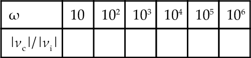
Explain why the table results show that an RC circuit acts as a high-cut filter and find the value of the high-cut frequency, defined as $f_{hc} = ω_{hc} / 2 π ? such ? that ? | υ_{c} |/| υ_{i} |=1 \sqrt{2.}$ $f_{hc} = ω_{hc} / 2 π ? such ? that ? | υ_{c} |/| υ_{i} |=1 \sqrt{2.}$

14.8. A spring of length, l has a mass m attached to it and a dashpot damping the motion. It is subject to a force f (t) forcing the motion as in Figure 14.2. The extension x₁ of the spring obeys the system of differential equations

$\frac{d}{d t} (\begin{array}{l} x_{1} \\ x_{2} \end{array}) ? = ? (\begin{array}{l} 0 & 1 \\ - k / m & - r / m \end{array}) ? (\begin{array}{l} x_{1} \\ x_{2} \end{array}) + ? (\begin{matrix} 0 \\ 1/ m \end{matrix}) ? f (t)$ $\frac{d}{d t} (\begin{array}{l} x_{1} \\ x_{2} \end{array}) ? = ? (\begin{array}{l} 0 & 1 \\ - k / m & - r / m \end{array}) ? (\begin{array}{l} x_{1} \\ x_{2} \end{array}) + ? (\begin{matrix} 0 \\ 1/ m \end{matrix}) ? f (t)$

By solving this system of equations, find the extension of the spring after time t in the following cases

(a) m = 1, r = 12, k = 11, f (t) = e^−2t, with initial extension 0 and 0 initial velocity.

(b) m = 2, r = 13, k = 20, f (t) = 10t,x₁(0) = 0 = x₂(0).

14.9. Solve the following difference equations

(a) $2 y_{n} - y_{n - 1} ? = ? - 3, ? y_{0} ? = ? 1$ $2 y_{n} - y_{n - 1} ? = ? - 3, ? y_{0} ? = ? 1$

(b) $4 y_{n} + y_{n - 1} = n, ? ? ? ? ? ? ? y_{0} ? = ? 2$ $4 y_{n} + y_{n - 1} = n, ? ? ? ? ? ? ? y_{0} ? = ? 2$

(c) $y_{n} - {1.2 y}_{n - 1} + {0.36 y}_{n - 2} ? = ? 4, ? y_{0} ? = ? 3, ? y_{1} ? = ? 2$ $y_{n} - {1.2 y}_{n - 1} + {0.36 y}_{n - 2} ? = ? 4, ? y_{0} ? = ? 3, ? y_{1} ? = ? 2$

(d) $y_{n} + 0.6 y_{n - 1} ? = ? 0.16 y_{n - 2} + {(0.5)}^{n}, ? ? ? ? y_{0} ? = ? 1, ? y_{1} = ? 2$ $y_{n} + 0.6 y_{n - 1} ? = ? 0.16 y_{n - 2} + {(0.5)}^{n}, ? ? ? ? y_{0} ? = ? 1, ? y_{1} = ? 2$

(e) $2 y_{n} + y_{n - 1} ? = ? cos (\frac{π n}{2}), ? ? ? ? ? ? ? y_{0} ? = ? 1.$ $2 y_{n} + y_{n - 1} ? = ? cos (\frac{π n}{2}), ? ? ? ? ? ? ? y_{0} ? = ? 1.$

..................Content has been hidden....................

You can't read the all page of ebook, please click here login for view all page.

Table of Contents for 14.6 Solving systems of differential equations

Create new playlist

Sign In

Sign Up

14.6 Solving systems of differential equations

Example 14.10

14.7 Difference equations

Example 14.11

System stability

14.8 Summary

14.9 Exercises

Table of Contents for
14.6 Solving systems of differential equations