Search in book...
Toggle Font Controls
Create new playlist

Name your new playlist

Playlist description (optional)
Sign In

Email address

Password

Forgot Password?

or

Continue with Facebook

Continue with Google
Sign Up

Full Name

Email address

Confirm Email Address

Password

or

Continue with Facebook

Continue with Google

Laplace and z transforms

15.1 Introduction

In this chapter, we will present a quick review of Laplace transform methods for continuous and piecewise continuous systems and z transform methods for discrete systems. The widespread application of these methods means that engineers need increasingly to be able to apply these techniques in multitudes of situations.

Laplace transforms are used to reduce a differential equation to a simple equation in s -space and a system of differential equations to a system of linear equations. We discover that in the case of zero initial conditions, we can solve the system by multiplying the Laplace transform of the input function by the transfer function of the system. Furthermore, if we are only interested in the steady state response, and we have a periodic input, we can find the response by simply adding the response to each of the frequency components of the input signal. In Chapter 16, we therefore look at finding the frequency components of a periodic function by finding its Fourier series.

Similar ideas apply to z transform methods applied to difference equations representing discrete systems.

The system transfer function is the Laplace transform of the impulse response function of the system. The impulse response is its response to an impulse function also called a delta function. Inputting an impulse function can be though of as something like giving the system a short kick to see what happens next. The impulse function is an idealized kick, as it lasts for no time at all and has energy of exactly 1. Because of these requirements, we find that the delta function is not a function at all, in the sense that we defined functions in Chapter 1. We find that it is the most famous example of a generalized function.

15.2 The Laplace transform – definition

The Laplace transform F(s) of the function f(t) defined for t > 0 is

$F (s) ? = ? \int_{0}^{\infty} e^{- s t} ? f (t) d t .$

The Laplace transform is a function of s where s is a complex variable. Because the integral definition of the Laplace transform involves an integral to∞ it is usually necessary to limit possible values of s so that the integral converges (i.e. does not tend to ∞). Also, for many functions the Laplace transform does not exist at all.

$L$ { } is the symbolic representation of the process of taking a Laplace transform (LT). Therefore,

$L {f (t)} ? = ? F (s) .$

Example 15.1

Find from the definition $L$ {e^3t}.

Solution

$L {e^{3 t}} ? = ? \int_{0}^{\infty} e^{3 t} ? e^{- s t} ? d t ? = ? \int_{0}^{\infty} e^{(3 - s) t} ? d t ? = ? {[\frac{e^{(3 - s) t}}{3 - s}]}_{0}^{\infty} .$

si20_e

Now e(3—s)t →0 as t →∞ only if the real part of (3 — s) is negative, that is, Re(s) > 3. Then the upper limit of the integration gives 0. Hence

$L {e^{3 t}} ? = ? \frac{1}{s ? - ? 3}$

si21_e

where Re{s} > 3.

Example 15.2

Find, from the definition, $L$ {cos(at)}.

Solution We need to find the integral

$I ? = ? \int_{0}^{\infty} e^{- s t} ? cos (a t) d t .$

We employ integration by parts twice until we find an expression that involves the original integral, I. We are then able to express I in terms of a and s.

Integrating by parts, using the formula ∫ u dv = uv – ∫ v du, where u =cos(at), dv =e^−st dt, du =−a sin(at) dt and v =e^−st I(−s), gives

$I ? = ? {[\frac{- e^{- s t}}{s} cos (a t)]}_{0}^{\infty} ? - ? \int_{0}^{\infty} \frac{e^{- s t}}{s} ? a ? sin (a t) d t .$

si24_e

The expression [e^−st cos(at)]∞ only has a finite value if e^−st→ 0 as t →∞. This will only be so if Re(s) > 0. With that proviso we get

$I ? = ? \frac{1}{s} ? - ? \frac{a}{s} ? \int_{0}^{\infty} ? e^{- s t} ? sin (a t) d t .$

si25_e

integrating the remaining integral on the right-hand side, again by parts, where this time u = sin(at), dv = e^−st dt, du = a cos(at) dt, v = e^−st /(–s). gives

$\begin{matrix} I ? = ? \frac{1}{s} ? {- [\frac{- a}{s^{2}} ? e^{- s t} ? sin (a t)]}_{0}^{\infty} ? - \frac{a^{2}}{s^{2}} ? \int_{0}^{\infty} e^{- s t} ? cos (a t) d t \\ = ? \frac{1}{s} ? - ? \frac{a^{2}}{s^{2}} ? \int_{0}^{\infty} ? e^{- s t} ? cos (a t) d t . \end{matrix}$

si26_e

We see that the remaining integral is the integral we first started with, which we called I. Hence

$I ? = ? \frac{1}{s} ? - ? \frac{a^{2}}{s^{2}} I$

si27_e

and solving this for I gives

$I (1 ? + ? \frac{a^{2}}{s^{2}}) ? = ? 1 / s, ? I ? = ? \frac{s}{s^{2} ? + ? a^{2}} .$

si28_e

So we have that

$L {cos (a t)} ? = ? \frac{s}{s^{2} ? + ? a^{2}}, ? where ? Re (s) ? > ? 0.$

15.3 The unit step function and the (impulse) delta function

The unit step function and delta function are very useful in systems theory.

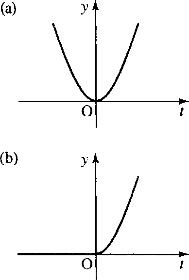
The unit step function

The unit step function is defined as follows:

$u (t) ? = ? {\begin{matrix} 1 & t \geq 0 \\ 0 & t < 0 \end{matrix}$

si30_e

and its graph is as shown in Figure 15.1.

f15-01-9780750658553 — Figure 15.1 The graph of the unit step function u(t).

The function is used to represent an idealized switch. It switches on at time t =0. If it is multiplied by any other function then it acts to switch that function on at t =0. That is, the function

$f (t) u (t) ? = ? {\begin{matrix} 0 & t < 0 \\ f (t) & t \geq 0. \end{matrix}$

An example for f(t) = t²is given in Figure 15.2.

f15-02-9780750658553 — Figure 15.2 Any function when multiplied by the unit step function is ‘switched on’ at t =0 (a) the function y =t²; (b) the function y =t² u(t).

As the Laplace transform only involves the integral from t =0, all functions can be thought of as multiplied by the unit step function because f(t) =f(t)u(t) as long as t > 0.

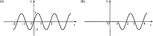
Shifting the unit step function

As we saw in Chapter 2, the graph of f (t – a) can be found by taking the graph of f(t) and moving it a units to the right. There is an example of a shifted unit step function in Figure 15.3.

f15-03-9780750658553 — Figure 15.3 (a) The graph of y =u(t). (b) The graph of y =u(t – 2) is found by shifting the graph of u(t) two units to the right.

Notice that the unit step function ‘switches on’ where the argument of u is zero. Multiplying any function by the shifted unit step function changes where it is switched on. That is

$f (t) u (t ? - ? a) ? = ? {\begin{matrix} 0 & t < a \\ f (t) & t \geq a . \end{matrix}$

The example of sin(t)u(t −1) is shown in Figure 15.4.

f15-04-9780750658553 — Figure 15.4 (a) The graph of sin(ωt). (b) The graph of u(t – 1) sin(ωt). Notice that this function is zero for t < 1 and equal to sin(ωt) for t > 1.

The delta function

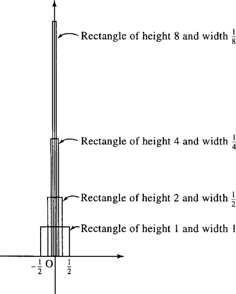
The impulse function, or delta function, is a mathematical representation of a kick. It is an idealized kick that lasts for no time at all and has energy of exactly 1.

The delta function, δ(t), is an example of a generalized function. A generalized function can be defined in terms of a sequence of functions. One way of defining it is as the limit of a rectangular pulse function, with area 1, as it halves in width and doubles in height. This sequence of functions is shown in Figure 15.5. Although the height of the pulse is tending to infinity, the area of the pulse remains 1.

f15-05-9780750658553 — Figure 15.5 The sequence of rectangular pulse functions of area 1. Starting from a pulse of height 1 and width 1 we double the height and half the width.

Two important properties of the delta function are

1. δ (t – a) = 0 for t ≠a,

2. $\int_{- \infty}^{\infty} δ (t) ? = ? 1.$

The second property expresses the fact that the area enclosed by the delta function is 1.

The unit step function, u(t), has no derivative at t = 0. Because of the sharp edges present in its graph and its jump discontinuity it is impossible to define a single tangent at that point. However, if we also consider the unit step function as a generalized function (by taking the limit of nice smooth, continuous curves as they approach the shape of the unit step function), we are able to define its derivative, which turns out to be the delta function. This gives the third definition

3. du /dt = δ(t).

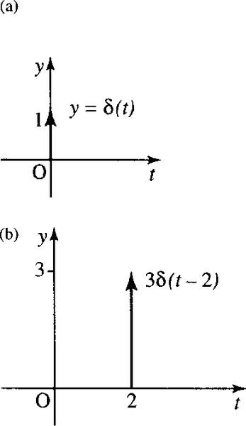
Symbolic representation of δ (t)

δ(t) can be represented on a graph by an arrow of height 1. The height represents the weight of the delta function. A shifted delta function, δ(t – a), is represented by an arrow at t = a. Examples are given in Figure 15.6.

f15-06-9780750658553 — Figure 15.6 Symbolic representations of delta functions: (a) δ(t); (b) 3δ(t – a).

15.4 Laplace transforms of simple functions and properties of the transform

Rather than finding a Laplace transform from the definition we usually use tables of Laplace transforms. A list of some common Laplace transforms is given in Table 15.1. We can then use the properties of the transform to find Laplace transforms of many other functions. To find the inverse transform, represented by $L^{- 1}$ { } we use the same table backwards. That is, look for the function of s on the right-hand column; the left-hand column then gives its inverse:

$\begin{matrix} F (s) ? = ? \int_{0}^{\infty} f (t) e^{- s t} d t & F (t) ? = ? L^{- 1} {F (s)} . \end{matrix}$

Table 15.1

Common Laplace transforms

f(t)	F(s) = £{f(t)}
u(t)	1/s	Re(s) > 0
δ(t)	1	Re(s) > 0
$\frac{t^{n - 1}}{(n - 1)!}$	$\frac{1}{s^{n}}$	Re(s) > 0
e^−at	$\frac{1}{s + a}$	Re(s) > −a
$\frac{1}{a} sin (a t)$	$\frac{1}{s^{2} + a^{2}}$	Re(s) > 0
cos(at)	$\frac{s}{s^{2} + a^{2}}$	Re(s) > 0
$\frac{1}{a} sinh (a t)$	$\frac{1}{s^{2} - a^{2}}$	Re(s) > \|a\|
cosh(at)	$\frac{s}{s^{2} - a^{2}}$	Re(s) > \|a\|

cetable1

Properties of the Laplace transform

In all of the following, F(s) = {f(t)}

1. Linearity:

$L {a f_{1} (t) ? + ? b f_{2} (t)} ? = ? a F_{1} (s) ? + ? F_{2} (s)$

where a and b are constants.

2. First translation (or Shift rule):

$L {e^{at} ? f (t)} ? = ? F (s ? - ? a)$

3. Second translation:

$L {f (t - a) u (t - a)} ? = ? e^{- a s} F (s) .$

4. Change of scale:

$L {f (a t)} = \frac{1}{a} F \frac{s}{a} .$

si39_e

5. Laplace transforms of derivatives:

$\begin{matrix} L {f' (t)} = s F (s) - f (0) \\ L {f ″ (t)} = s^{2} F (s) - s f (0) - f' (0) \end{matrix}$

si40_e

and

$L {f^{(n)} (t)} ? = ? s^{n} F (s) ? - ? s^{n - 1} f (0) ? - ? \dots - s f^{(n - 2)} (0) ? - ? f^{(n - 1)} (0)$

6. Integrals:

$L {\int_{0}^{t} f (τ) d τ} ? = ? \frac{F (s)}{s} .$

si42_e

7. Convolution:

$L {f ? * ? g} ? = ? L ? {\int_{0}^{t} f (τ) g (t - τ) d τ} ? = ? F (s) G (s) .$

si43_e

8. Derivatives of the transform:

$L {t^{n} f (t)} ? = ? {(- 1)}^{n} F^{(n)} (s)$

where

$F^{n} (s) ? = ? \frac{d^{n} F^{(n)}}{d s^{n}} (s) .$

si45_e

Example 15.3

(Linearity) Find $L$ {3t²+ sin(2t)}.

Solution From Table 15.1

$L {\frac{t^{2}}{2}} ? = ? \frac{1}{s^{3}}$

and

$L {\frac{sin (2 t)}{2}} ? = ? \frac{1}{(s^{2} + 4)} .$

si48_e

Therefore

$L {3 t^{2} ? + ? sin (2 t)} ? = ? 6 L {\frac{t^{2}}{2}} ? + ? 2 L {\frac{sin (2 t)}{2}} ? = ? \frac{6}{s^{3}} ? + ? \frac{2}{s^{2} + 4}$

si49_e

using

$L {a f_{1} (t) ? + ? b f_{2} (t)} ? = ? a F_{1} (s) ? + ? b F_{2} (s) .$

Example 15.4

(Linearity and the inverse transform) Find

$L^{- 1} {\frac{2}{s + 4} ? + ? \frac{4 s}{s^{2} + 9}}$

si51_e

Solution From Table 15.1

$L^{- 1} {\frac{1}{s + 4}} = e^{- 4 t}$

si52_e

and

$L^{- 1} {\frac{s}{s^{2} + 9}} = cos (3 t)$

si53_e

Therefore

$L^{- 1} {\frac{2}{s + 4} + \frac{4 s}{s^{2} + 9}} = 2 e^{- 4 t} + 4 cos (3 t)$

si54_e

Example 15.5

(First translation) Find $L$ {t²e^−3t}.

Solution As

$L {t^{2}} = \frac{2}{s^{3}}$

using

$L {e^{- a t} f (t)} = F (s - a) .$

Then multiplying by e^−3t in the t domain will shift the function F (s) by 3:

$L {t^{2} e^{- 3 t}} = \frac{2}{{(s + 3)}^{2}}$

si58_e

Example 15.6

(First translation – inverse transform) Find

$L^{- 1} {\frac{s + 2}{{(s + 2)}^{2} + 9}} .$

Solution As

$L^{- 1} {\frac{s}{s^{2} + 9}} = cos (3 t)$

and as

$\frac{s + 2}{{(s + 2)}^{2} + 9}$

is s / (s² + 9) translated by 2, using the first translation rule this will multiply in the t domain by e ^−2t so

$L^{- 1} {\frac{s + 2}{{(s + 2)}^{2} + 9}} = cos (3 t) e^{- 2 t}$

Example 15.7

(Second translation) Find the Laplace transform of

$f (t) = {\begin{array}{l} 0 & t < \frac{2}{3} \\ sin (3 t - 2) & t \geq \frac{2}{3} \end{array}$

si63_e

Solution f (t) can be expressed using the unit step function

$f (t) = \sin (3 t - 2) u (t - \frac{2}{3}) = \sin (3 (t - \frac{2}{3})) u (t - \frac{2}{3}) .$

Using $L$ {f(t – a)u(t –a)} =e^−as F(s) and as

$L {\sin (3 t)} = \frac{3}{s^{2} + 9}$

we have

$\sin (3 (t - \frac{2}{3})) u (t - \frac{2}{3}) = \frac{3 e^{- 2 s / 3}}{s^{2} + 9}$

Example 15.8

(Second translation – inverse transform) Find

$L^{- 1} {\frac{e^{- s}}{(s + 2) ?^{2}}} .$

si68_e

Solution As

$L^{- 1} {\frac{1}{(s + 2) ?^{2}}} = t e^{- 2 t}$

si69_e

(using first translation), the factor of e^−s will translate in the t domain, t → t −1. Then

$L^{- 1} {\frac{e^{- s}}{(s + 2) ?^{2}}} = (t - 1) e^{- 2 (t - 1)} u (t - 1)$

si70_e

by second translation.

Example 15.9

(Change of scale) Given

$L {cos (t)} = \frac{s}{s^{2} + 1}$

find $L$ {cos(3t)}using the change of scale property of the Laplace transform

$L {f ? (a t)} = \frac{1}{a} F \frac{s}{a} .$

Solution As

$L {cos (t)} = \frac{s}{s^{2} + 1} = F (s)$

to find cos(3t) we put a =3 into the change of scale property

$L {f (a t)} = \frac{1}{a} F \frac{s}{a}$

giving

$L {cos (3 t)} = \frac{1}{3} \frac{s / 3}{(s / 3) ?^{2} + 1} = \frac{s}{s^{2} + 9}$

si76_e

Example 15.10

(Derivatives) Given

$L {cos (2 t)} = \frac{s}{s^{2} + 4}$

find {sin(2t)} using the derivative rule.

Solution If f(t) = cos(2t) then f′(t) =– 2sin(2t):

$L {cos (2 t)} = \frac{s}{s^{2} + 4}$

and f(0) =cos(0) = 1. From the derivative rule $L$ {f′(t)} = sF(s) –f(0),

$L {- 2 sin (2 t)} = s (\frac{s}{s^{2} + 4}) - 1 = \frac{s^{2}}{s^{2} + 4} - 1 = \frac{s^{2} - s^{2} - 4}{s^{2} + 4} = \frac{- 4}{s^{2} + 4} .$

By linearity,

$L {sin (2 t)} = \frac{1}{- 2} (\frac{- 4}{s^{2} + 4}) = \frac{2}{s^{2} + 4} .$

Example 15.11

(Integrals) Using

$L ? {\int_{0}^{t} f (τ) d τ} = \frac{F (s)}{s}$

and

$L {t^{2}} = \frac{2}{s^{3}}$

find

$L ? {\frac{t^{3}}{3}} .$

Solution As

$\int_{0}^{t} τ^{2} d τ = [\frac{τ^{3}}{3}] ?_{0}^{t} = \frac{t^{3}}{3}$

and

$L {t^{2}} = \frac{2}{s^{3}}$

then

$L ? {\int_{0}^{t} τ^{2} d τ} = \frac{2 / s^{3}}{s} = \frac{2}{s^{4}} ? \Rightarrow ? L ? {\frac{t^{3}}{3}} = \frac{1}{s} (\frac{2}{s^{3}}) = \frac{2}{s^{4}} .$

Example 15.12

(Convolution) Find

$L^{- 1} {\frac{1}{(s - 2) (s - 3)}}$

using the convolution property:

$L ? {\int_{0}^{1} f (t) g (t - τ) d τ} = F (s) G (s) .$

Solution

$\frac{1}{(s - 2) (s - 3)} = \frac{1}{(s - 2)} \frac{1}{(s - 3)} .$

Therefore, call

$F (s) = \frac{1}{s - 2}, ? G (s) = \frac{1}{s - 3}$

$f (t) = L^{- 1} {\frac{1}{s - 2}} = e^{2 t}$

$g (t) = L^{- 1} {\frac{1}{s - 3}} = e^{3 t} .$

Then by the convolution rule

$L^{- 1} {\frac{1}{(s - 2) (s - 3)}} = \int_{0}^{t} e^{2 τ} e^{3 (t - τ)} d τ .$

This integral is an integral over the variable τ. t is a constant as far as the integration process is concerned. We can use the properties of powers to separate out the terms in τ and the terms in t, giving

$\begin{matrix} ℒ^{- 1} {\frac{1}{(s - 2) (s - 3)}} = e^{3 t} \int_{0}^{t} e^{- τ} d τ = e^{3 t} {[\frac{e^{- τ}}{- 1}]}_{0}^{t} \\ = e^{3 t} (- e^{- t} + 1) \\ = - e^{2 t} + e^{3 t} . \end{matrix}$

si95_e

Example 15.13

(Derivatives of the transform) Find $L$ {t sin(3t)}.

Solution Using the derivatives of the transform property

$L {t^{n} f (t)} = (- 1) ?^{n} F^{(n)} (s)$

we have f(t) = sin(3t) and

$L {sin (3 t)} = \frac{3}{s^{2} + 9} = F (s)$

(from Table 15.1).

As sin(3t) is multiplied by t in the expression to be transformed, we use the derivative of the transform property with n = 1:

$L {t^{1} f (t)} = (- 1) ?^{1} F^{(1)} (s) = - F' (s)$

to give

$L {t ? sin (3 t)} = - \frac{d}{d s} (\frac{3}{s^{2} + 9}) = \frac{6 s}{(s^{2} + 9) ?^{2}} .$

Example 15.14

(Derivatives of the transform and the inverse transform) Find

$L^{- 1} {\frac{s}{(s^{2} + 4) ?^{2}}}$

si101_e

Solution We notice that

$\frac{s}{(s^{2} + 4) ?^{2}} = - \frac{1}{2} \frac{d}{d s} (\frac{1}{s^{2} + 4}) .$

si102_e

Using the derivatives of the transform property

$L {t^{n} f (t)} = (- 1) ?^{n} F^{(n)} (s)$

and setting n =1 we have

$L^{- 1} {(- 1) d F / d s} = t f (t)$

and as

$L^{- 1} {\frac{1}{(s^{2} + 4)}} = \frac{1}{2} sin (2 t)$

si105_e

we have

$L^{- 1} {\frac{s}{(s^{2} + 4) ?^{2}}} = \frac{1}{2} t (\frac{1}{2} sin (2 t)) = \frac{t}{4} sin (2 t)$

si106_e

Using partial fractions to find the inverse transform

Partial fractions can be used to find the inverse transform of expressions like

$\frac{11 s + 7}{s^{2} - 1}$

si107_e

by expressing F (s) as a sum of fractions with a simple factor in the denominator.

Example 15.15

Find the inverse Laplace transform of

$\frac{11 s + 7}{s^{2} - 1}$

si108_e

Solution Factorize the denominator. This is equivalent to finding the values of s for which the denominator is 0, because if the denominator has factors s_l and s₂ we know that we can write it as c(s – s_l) (s –s₂) where c, is some number. In this case we could solve for s² – 1 =0. However, it is not difficult to spot that s²–1 =(s −1) (s + 1). The values for which the denominator is zero are called the poles of the function.

$\frac{11 s + 7}{s^{2} - 1} = \frac{11 s + 7}{(s - 1) (s + 1)} .$

si109_e

We assume that there is an identity such that

$\frac{11 s + 7}{(s^{2} - 1)} = \frac{A}{s - 1} + \frac{B}{s + 1} .$

Multiply both sides of the equation by (s –1) (s + 1) to get

$11 s + 7 = A (s + 1) + B (s - 1) .$

$\begin{array}{l} Substitute s = 1; then 11 + 7 = 2 A \Rightarrow A = 9. \\ Substitute s = - 1; then - 11 ? + ? 7 = - 2 B \Rightarrow B = 2. \end{array}$

si112_e

$ℒ^{- 1} {\frac{11 s + 7}{s^{2} - 1}} = ℒ^{- 1} {\frac{9}{s - 1} + \frac{2}{s + 1}} = 9 e^{t} + 2 e^{- t} .$

si113_e

A quick formula for partial fractions

There is a quick way of getting the partial fractions expansion, called the ‘cover up’ rule, which works in the case where all the roots of the denominator of F(s) are distinct. If F(s) = P(s)/ Q(s) then write Q(s) in terms of its factors Q (s)

$Q (s) = c (s - s_{1}) (s - s_{2}) (s - s_{3}) \dots (s - s_{r}) \dots (s - s_{n})$

where s_l … s_nare its distinct roots. Then we can find the constant A_r, etc., for the partial fraction expansion from covering up each of the factors of Q in term and substituting s = s _r in the rest of the expression:

$F (s) = \frac{P (s)}{c (s - s_{1}) (s - s_{2}) (s - s_{3}) \dots (s - s_{r}) \dots (s - s_{n})}$

si115_e

then

$F (s) = \frac{A_{1}}{(s - s_{1})} + \frac{A_{2}}{(s - s_{2})} + \dots + \frac{A_{r}}{(s - s_{r})} + \dots + \frac{A_{n}}{(s - s_{n})}$

si116_e

where

In this case

$F (s) = \frac{11 s + 7}{s^{2} - 1} = \frac{11 s + 7}{(s - 1) (s + 1)} = \frac{A}{s - 1} + \frac{B}{s + 1}$

si117_e

Then A is found by substituting s =1 into

and B is found by substituting s = −1 into

This gives the partial fraction expansion, as before, as

$F (s) = \frac{9}{s + 1} + \frac{2}{s - 1} .$

si118_e

This method can also be used for complex poles; for instance,

$\frac{1}{(s^{2} + 4) (s + 3)} = \frac{1}{(s + 3) (s - j 2) (s - j 2)} .$

si119_e

The roots of the denominator are −3, j2 and –j2, so we get for the partial fraction expansion

$\begin{matrix} \frac{1}{(s^{2} + 4) (s + 3)} = \frac{1}{13 (s + 3)} + \frac{1}{(- 8 + j 12) (s - j 2)} \\ + \frac{1}{(- 8 - j 12) (s + j 2)} . \end{matrix}$

si120_e

The inverse transform can be found directly or the last two terms can be combined to give the expansion as

$\frac{1}{(s^{2} + 4) (s + 3)} = \frac{1}{13 (s + 3)} + \frac{- 16 s + 48}{208 (s^{2} + 4)} = \frac{1}{13 (s + 3)} + \frac{3 - s}{13 (s^{2} + 4)} .$

si121_e

Repeated poles

If there are repeated factors in the denominator, for example,

$\frac{4}{{(s + 1)}^{2} (s - 2)}$

si122_e

then try a partial fraction expansion of the form

$\frac{4}{{(s + 1)}^{2} (s - 2)} = \frac{A}{{(s + 1)}^{2}} + \frac{B}{s + 1} + \frac{C}{s - 2} .$

si123_e

The ‘cover up’ rule cannot be used to find the coefficients A and B.

15.5 Solving linear differential equations with constant coefficients

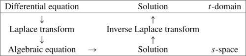
The scheme for solving differential equations is as outlined below. The Laplace transform transforms the linear differential equation with constant coefficients to an algebraic equation in s. This can be solved and then the inverse transform of this solution gives the solution to the original differential equation.

Example 15.16

A d.c. voltage of 3 V is applied to an RC circuit with R = 2000 Ω and C = 0.001 F, where q(0) =0. Find the voltage across the capacitor as a function of t.

Solution From Kirchoff's voltage law, we get the differential equation

$\begin{array}{l} 2000 \frac{d q}{d t} + \frac{q}{0.001} = 3 \\ \frac{d q}{d t} + 0.5 q = 0.0015 \end{array}$

si124_e

Taking Laplace transforms of both sides of the equation where Q(s) = $L$ {q(t)},

$s Q (s) - q (0) + 0.5 Q (s) = \frac{0.0015}{s} .$

Here, we have used the derivative property of the Laplace transform, q′ (t) = s Q (s)– q (0). Solve the algebraic equation

$(s + 0.5) Q = \frac{0.0015}{s} \Leftrightarrow Q = \frac{0.0015}{s (s + 0.5)} .$

si127_e

We need to find the inverse Laplace transform of this function of s so that we expand using partial fractions, giving

$\begin{matrix} Q = \frac{0.003}{s} - \frac{0.003}{s + 0.5} \\ q = ℒ^{- 1} {\frac{0.003}{s} - \frac{0.003}{s + 0.5}} = 0.003 - 0.003 e^{- 0.5 t} . \end{matrix}$

si128_e

The voltage across the capacitor is

$\frac{q (t)}{c} = \frac{0.003 - 0.003 e^{- 0.5 t}}{0.001} = 3 (1 - e^{- 0.5 t}) .$

si129_e

Example 15.17

Solve the following differential equation using Laplace transforms:

$\frac{d^{2} x}{d t^{2}} + 4 \frac{d x}{d t} + 3 x = e^{- 3 t}$

given x(0) = 0.5 and dx(0)/dt= − 2.

Solution Transform the differential equation

$\frac{d^{2} x}{d t^{2}} + 4 \frac{d x}{d t} + 3 x = e^{- 3 t}$

si131_e

to get

$(s^{2} X (s) - s x (0) - \frac{d x}{d t} (0)) + 4 (s X (s) - x (0)) + 3 X (s) = \frac{1}{s + 3} .$

si132_e

Here we have used

$L {\frac{d^{2}}{d t^{2}}} = s^{2} X (s) - s x (0) - \frac{d x}{d t} (0)$

si133_e

and

$L {\frac{d x}{d t}} = s X (s) - x (0) .$

si134_e

Substitute x (0) = 0.5 and dx (0) / dt = – 2

$\begin{array}{l} s^{2} X (s) - \frac{1}{2} s + 2 + 4 s X (s) - 2 + 3 X (s) = \frac{1}{s + 3} \\ \Leftrightarrow ? ? ? ? X (s) (s^{2} + 4 s + 3) = \frac{1}{s + 3} + \frac{1}{2} s \\ \Leftrightarrow ? ? ? ? X (s) = \frac{1}{(s + 3) (s^{2} + 4 s + 3)} + \frac{s}{2 (s^{2} + 4 s + 3)} \end{array}$

si135_e

Use partial fractions:

$\begin{array}{l} \frac{1}{(s + 3) (s^{2} + 4 s + 3)} = \frac{1}{(s + 3) (s + 3) (s + 1)} \\ \frac{1}{(s + 3) (s + 3) (s + 1)} = \frac{A}{(s + 3)} + \frac{B}{{(s + 3)}^{2}} + \frac{C}{s + 1} \\ \Rightarrow ? ? ? ? 1 = A (s + 3) (s + 1) + B (s + 1) + C {(s + 3)}^{2} . \end{array}$

si136_e

Substituting s = −3

$1 = - 2 B ? ? \Leftrightarrow ? ? B = - \frac{1}{2} .$

si137_e

Substituting s = −1

$1 = 4 C ? ? \Leftrightarrow ? ? C = \frac{1}{4} .$

si138_e

Substituting s = 0

$1 = 3 A + B + 9 C .$

Substituting $B = - \frac{1}{2} ? a n d ? C = \frac{1}{4}$ gives

$1 = 3 A - \frac{1}{2} + \frac{9}{4} ? ? ? ? \Leftrightarrow ? ? ? ? A = - \frac{1}{4} .$

Therefore

$\frac{1}{{(s + 3)}^{2} (s + 1)} = - \frac{1}{4 (s + 3)} - \frac{1}{2 {(s + 3)}^{2}} + \frac{1}{4 (s + 1)} .$

si142_e

We can use the ‘cover up’ rule to find

$\frac{s}{2 (s + 3) (s + 1)} = \frac{3}{4 (s + 3)} - \frac{1}{4 (s + 1)}$

si143_e

so that

$\begin{array}{l} X (s) & = & - \frac{1}{4 (s + 3)} - \frac{1}{2 {(s + 3)}^{2}} + \frac{1}{4 (s + 1)} + \frac{3}{4 (s + 3)} \\ - \frac{1}{4 (s + 1)} \\ = & \frac{- 1}{2 {(s + 3)}^{2}} + \frac{1}{2 (s + 3)} . \end{array}$

si144_e

Taking the inverse transform, we find

$x (t) = - \frac{1}{2} t e^{- 3 t} + \frac{1}{2} e^{- 3 t} = \frac{e^{- 3 t}}{2} (1 - t)$

si145_e

15.6 Laplace transforms and systems theory

The transfer function and impulse response function

An important role is played in systems theory by the impulse response function, the Laplace transform of which is called the Transfer Function (or system function). We remember from Chapter 14 that a linear, time-invariant system is represented by a linear differential equation with constant coefficients. We will stick to second-order equations although the results can be generalized to any order.

An LTI system can be represented by

$a \frac{d^{2} y}{d t^{2}} + b \frac{d y}{d t} + c y = f (t) .$

si146_e

If we take f(t) as the delta function δ(t) then we get

$a \frac{d^{2} y}{d t^{2}} + b \frac{d y}{d t} + c y = δ (t) .$

si147_e

By definition of the impulse response function we consider all initial conditions to be 0.

Taking the Laplace transform we get

$\begin{array}{l} a s^{2} Y (s) + b s Y (s) + c Y (s) = 1 \\ Y (s) (a s^{2} + b s + c) = 1 \\ Y (s) = \frac{1}{a s^{2} + b s + c} . \end{array}$

si148_e

Notice that the poles of this function are found by solving as²+bs+c = 0, which we recognize as the auxiliary equation or characteristic equation from Chapter 14.

This function, the Laplace transform of the impulse response function, is called the transfer function and is usually denoted by H(s), so we have

$H (s) = \frac{1}{a s^{2} + b s + c}$

si149_e

and $L$ {H(s)} = h(t), where h(t) is the impulse response function.

Note that the impulse response function describes the behaviour of the system after it has been given an idealized kick.

Example 15.18

Find the transfer function and impulse response of the system described by the following differential equation:

$3 \frac{d y}{d t} + 4 y = f (t) .$

Solution To find the transfer function replace f(t) by δ(t) and take the Laplace transform of the resulting equation assuming zero initial conditions:

$3 \frac{d y}{d t} + 4 y = δ (t) .$

si152_e

Taking the Laplace transform of both sides of the equation we get

$\begin{array}{l} 3 (s Y - y (0)) + 4 Y = 1 \\ A s ? y (0) = 0, \\ Y = \frac{1}{3 s + 4} = H (s) . \end{array}$

si153_e

To find the impulse response function we take the inverse transform of the transfer function to find

$h (t) = L^{- 1} {\frac{1}{3 s + 4}} = e^{\frac{- 4 t}{3} .}$

si154_e

We now discover that we can find the system response to any input function f(t), with zero initial conditions, by using the transfer function.

Response of a system with zero initial conditions to any input f(t)

Assuming all initial conditions are zero, that is, y′ (0) = 0 and y (0) = 0, then the equation

$a \frac{d^{2} y}{d t^{2}} + b \frac{d y}{d t} + c y = f (t)$

si155_e

transforms to become

$(a s^{2} + b s + c) Y (s) = F (s) ? ? ? ? \Leftrightarrow ? ? ? ? Y (s) = \frac{F (s)}{a s^{2} + b s + c} .$

si156_e

We have just discovered that the transfer function, H (s), is given by

$H (s) = \frac{1}{a s^{2} + b s + c} .$

si157_e

Then we find that

$Y (s) = F (s) H (s) .$

In order to find the response of the system to the function f(t) we take the inverse transform of this expression. We are able to use the convolution property of Laplace transforms which states:

$L {\int_{0}^{t} ? ? f (τ) g (t - τ) d τ} = F (s) G (s)$

si159_e

or equivalently

$L^{- 1} {F (s) G (s)} = \int_{0}^{t} ? ? f (τ) g (t - τ) d τ .$

si160_e

The integral ∫^t₀ f(t) g(t – τ) dτ is called the convolution of f and g and can be expressed as f(t) * g(t). So we find that the response of the system with zero initial conditions to any input function f(t) is given by the convolution of f(t) with the system's impulse response:

$y (t) = L^{- 1} {F (s) H (s)} = f (t) * h (t) .$

We can use this result to solve two types of problems, given zero initial conditions. If we know the impulse response function of the system then we can find the system response to any input f(t) either by convolving in the time domain y(t) = f(t) ∗ h(t) or by finding the Laplace transform of f (t), F(s), and finding the transfer function of the system $L$ {h (t)} = H(s) and then finding Y(s) = H (s) F (s) and taking the inverse transform of this to find y (t). This type of problem is called a convolution problem. The other type of problem is that given any output, y(t), and given the input, f(t), we can deduce the impulse response of the system. This we do by finding F(s) = $L$ {f(t)}, Y(s) = $L$ {y(t)} and then H(s) = Y (s) / F (s), thus giving the transfer function. To find the impulse response we find h(t) = $L$ ^-l{H(s)}

Example 15.19

The impulse response of a system is known to be h(t) = e^3t. Find the response of the system to an input of f(t) = 6 cos(2t) given zero initial conditions.

Solution Method 1. We can take Laplace transforms and use Y(s)) = H(s)F(s). In this case

$\begin{array}{l} h (t) = e^{3 t} \Leftrightarrow H (s) = L {e^{3 t}} = \frac{1}{s - 3} \\ f (t) = 6 cos (2 t) \Leftrightarrow F (s) = L {6 cos (2 t)} = \frac{6 s}{4 + s^{2}} . \end{array}$

si166_e

Hence

$Y (s) = H (s) F (s) = \frac{6 s}{(s - 3) (4 + s^{2})} .$

si167_e

As we want to find y(t), we use partial fractions:

$\begin{matrix} \frac{6 s}{(s - 3) (4 + s^{2})} & = \frac{6 s}{(s - 3) (s + j 2) (s - j 2)} \\ = \frac{18}{13 (s - 3)} + \frac{3}{(j 2 - 3) (s - j 2)} \\ - \frac{3}{(j 2 + 3) (s + j 2)} ? ? ? ? (using ? the ? ‘ cover ? up ’ ? rule) \\ = \frac{18}{13 (s ? - ? 3)} - \frac{3 (6 s - 8)}{13 (s^{2} + ? 4)} \\ = \frac{18}{13 (s ? - ? 3)} - \frac{18 s}{13 (s^{2} + ? 4)} + \frac{12}{13} \frac{2}{(s^{2} + 4)} . \end{matrix}$

si168_e

We can now take the inverse transform to find the system response:

$\begin{matrix} ? & y (t) = L^{- 1} {Y (s)} \\ = L^{- 1} {\frac{18}{13 (s - 3)} - \frac{18 s}{13 (s^{2} + 4)} + \frac{12}{13} \frac{2}{(s^{2} + 4)}} \\ = \frac{18}{13} e^{3 t} - \frac{18}{13} cos (2 t) + \frac{12}{13} sin (2 t) . \end{matrix}$

si169_e

Alternative method. Find y(t) by taking the convolution of f(t) with the impulse response function

$y (t) = f (t) * h (t) = (6 cos (2 t)) * (e^{3 t})$

By definition of convolution

$(6 cos (2 t)) * (e^{3 t}) = \int_{0}^{t} ? ? 6 cos (2 τ) e^{3 (t - τ)} d τ .$

si171_e

As this is a real integral we can use the trick of writing cos(2τ) = Re(e^j2τ) to make the integration easier. So we find

$\begin{matrix} I = \int_{0}^{t} 6 e^{j 2 τ} e^{3 (t - τ)} d τ \\ = 6 e^{3 t} \int_{0}^{t} e^{τ (j 2 - 3)} d τ \\ = 6 e^{3 t} {[\frac{e^{t (j 2 - 3)}}{j 2 - 3}]}_{0}^{t} \\ = 6 e^{3 t} (\frac{e^{t (j 2 - 3)}}{j 2 - 3} - \frac{1}{j 2 - 3}) \\ = \frac{6 e^{3 t} (- j 2 - 3) (e^{- 3 t} (cos (2 t) + j ? sin (2 t)) - 1) .}{4 + 9} \end{matrix}$

si172_e

Taking the real part of this result we get the system response as

$\begin{matrix} \int_{0}^{t} 6 cos (2 τ) e^{3 (t - τ)} d τ = \frac{6}{13} (- 3 cos (2 t) + 2 sin (2 t)) + \frac{18}{13} e^{3 t} \\ = - \frac{18}{13} cos (2 t) + \frac{12}{13} sin (2 t) + \frac{18}{13} e^{3 t} \end{matrix}$

si173_e

which confirms the result of the first method.

Example 15.20

A system at rest has a constant input of f(t) = 3 applied at t = 0. The output is found to be $u (t) (\frac{3}{2} - \frac{3}{2} e^{- 2 t})$ si174_e . Find the impulse response of the system.

Solution Since

$y (t) = u (t) (\frac{3}{2} - \frac{3}{2} e^{- 2 t})$

we have

$y (s) = \frac{3}{2 s} - \frac{3}{2 (s + 2)} = \frac{3 s + 6 - 3 s}{2 s (s + 2)} = \frac{3}{s (s + 2)}$

si176_e

and as f(t) = 3, we have

$F (s) = \frac{3}{s} .$

si177_e

Hence

$H (s) = \frac{Y (s)}{F (s)} = \frac{3 / (s (s + 2))}{3 / s} = \frac{1}{s + 2}$

si178_e

giving

$h (t) = L^{- 1} {\frac{1}{s + 2}} = e^{- 2 t} .$

si179_e

Hence the impulse response is h (t) = e^−2t.

The frequency response

In this section, we shall seek to establish a relationship between the transfer function and the steady state response to a single frequency input. Consider the response of the system

$\ddot{y} + 3 \dot{y} + 2 y = f (t)$

to a single sinusoidal input e^j^ωt= cos(ωt) + j sin(ωt) with y(0) = 2 and Ý(0) = 1. Taking Laplace transforms we find

$\begin{array}{l} s^{2} Y - 2 s - 1 + 3 (s Y - 2) + 2 Y = \frac{1}{s - j ω} \\ Y (s^{2} + 3 s + 2) = 2 s + 7 + \frac{1}{s - ω} \\ Y = \frac{2 s + 7}{s^{2} + 3 s + 2} + \frac{1}{(s - j ω) (s^{2} + 3 s + 2)} . \end{array}$

si181_e

Remember

$\begin{matrix} H (s) = \frac{1}{s^{2} + 3 s + 2} = \frac{1}{(s + 2) (s + 1)} \\ Y = \frac{2 s + 7}{(s + 2) (s + 1)} + \frac{1}{(s - j ω) (s + 2) (s + 1)} . \end{matrix}$

si182_e

The first term in this expression is due to non-zero initial conditions. We are particularly interested in the second term in the expression for Y(s), which we notice may be written as H(s)/(s – jω).

Using the ‘cover up’ rule to write Y(s) in its partial fractions,

$Y (s) = \frac{5}{s + 1} - \frac{3}{s + 2} + \frac{1}{(- 1 - j ω) (s + 1)} + \frac{1}{(2 + j ω) (s + 2)} + \frac{H (j ω)}{s - j ω} .$

si183_e

Taking inverse transforms we find

$Y (t) = 5 e^{- t} - 3 e^{- 2 t} + \frac{1}{- 1 - j ω} e^{- t} + \frac{1}{2 + j ω} e^{- 2 t} + H (j ω) e^{j ω t} .$

si184_e

The first two terms in this expression are caused by the non-zero initial values and decay exponentially. The next two terms also decay with increasing t and are as a result of the abrupt turn on of the input at t = 0. Thus for a stable system, all four terms are part of the transient solution that dies out as t increases. The fifth and final term is the sinusoidal input f(t) = e^jωt multiplied by H(jω). H(jω) is a complex constant. This is the steady state response of the system to a single sinusoidal input, which we have shown in this case is given by

$Y (t) = H (j ω) e^{j ω t} .$

We can then see that for a single sinusoid input the steady state response is found by substituting s = jω into the transfer function for the system and multiplying the resulting complex constant by the sinusoidal input. In other words, the steady state response is a scaled and phase shifted version of the input. We can find the response to a sine or cosine input by

$y (t) = Re (H (j ω) e^{j ω t}) ? ? ? ? for ? ? f (t) = cos (ω t)$

and

$y (t) = Im (H (j ω) e^{j ω t}) ? ? ? ? for ? ? f (t) = sin (ω t)$

Alternatively, we can find the response to e^jωt and to e^−jωt and use the fact that

$\begin{matrix} cos (ω t) = \frac{1}{2} (e^{j ω t} + e^{- j ω t}) \\ sin (ω t) = \frac{1}{2 j} (e^{j ω t} - e^{- j ω t}) \end{matrix}$

si188_e

to write

$\begin{matrix} for ? ? f (t) = cos (ω t), ? ? ? ? y (t) = \frac{1}{2} (H (j ω) e^{j ω t} + H (- j ω) e^{- j ω t}) \\ for ? ? f (t) = sin (ω t), ? ? ? ? y (t) = \frac{1}{2 j} (H (j ω) e^{j ω t} - H (- j ω) e^{- j ω t}) . \end{matrix}$

si189_e

All of these results make use of the principle of superposition for linear systems.

We have seen in this section that the response to a simple sinusoid can be characterized by multiplying the input by a complex constant H(jω) where ω is the angular frequency of the input. The function H(jω) is called the frequency response function. It is this result that motivates us towards the desirability of expressing all signals in terms of cosines and sines of single frequencies – a technique known as Fourier analysis. We shall look at Fourier Analysis for periodic functions in Chapter 16.

Example 15.21

A system transfer function is known to be

$H (s) = \frac{1}{3 s + 1}$

si190_e

then find the steady state response to the following:

(a) f(t) = e^j^2t;

(b) f(t) = 3 cos(2t).

Solution (a) The steady state response to a single frequency e^jωt is given H(jω)e^jωt. Here f(t) = e^j2t, so in this case ω = 2 and H(s) is given as 1/(3s + 1). Hence we get the steady state response as

$H (j 2) e^{j 2 t} = \frac{1}{3 (j 2) + 1} e^{j 2 t} = \frac{e^{j 2 t}}{1 + j 6} = \frac{(1 - j 6) e^{j 2 t}}{37}$

si191_e

(b) Using (1/2)(H(jω)e^jωt + H(−jω)e-^j^ωt) as the response to cos(ωt) and substituting for Hand ω = 2 gives

$\begin{matrix} \frac{1}{2} (\frac{(1 - 6 j) e^{j 2 t}}{37} + \frac{(1 + j 6)}{37} e^{- j 2 t}) \\ = \frac{1}{74} ((1 - j 6) (cos (2 t) + j ? sin (2 t))) \\ \begin{array}{l} + (1 + j 6) (cos (2 t) - j ? sin (2 t)) \\ = \frac{1}{37} (cos (2 t) + 6 ? sin (2 t)) . \end{array} \end{matrix}$

si192_e

Hence, the steady state response to an input of 3 cos(2t) is

$\frac{3}{37} (cos (2 t) + 6 ? sin (2 t)) .$

si193_e

15.7 z transforms

z transforms are used to solve problems in discrete systems in a manner similar to the use of Laplace transforms for piecewise continuous systems. We take z transforms of sequences. We shall assume that our sequences begin with the zeroth term and have terms for positive n. f₀, f₁ f₂,..,f_n,. is an input sequence to the system. However, when considering the initial conditions for a difference equation it is convenient to assign them to y_–j, …, y₋₂, y₋₁ etc., where j is the order of the difference equation. So, in that case, we shall allow some elements in the sequence with negative subscript. Our output sequence will be of the form y_−j, …, y₋₂ y₋₁, y₀, y₁, y₂,…, y_n, where the difference equation describing the system only holds for n ≥ 0.

z transform definition

The z transform of a sequence f₀, f₁ f₂,…, f_n,… is given by

$F (z) = \sum_{n = 0}^{\infty} f_{n} z^{- n} .$

si194_e

As this is an infinite summation it will not always converge. The set of values of z for which it exists is called the region of convergence. The sequence, f₀, f₁ f₂,…, f_n,… is a function of an integer, however, its z transform is a function of a complex variable z. The operation of taking the z transform of the sequence f_n is represented by Z{f_n} = F(z).

Example 15.22

Find the z transform of the finite sequence 1, 0, 0.5,3.

Solution We multiply the terms in the sequence by z^—n, where n = 0, 1, 2, … and then sum the terms, giving

$F (z) = 1 + 0 z^{- 1} + 0.5 z^{- 2} + 3 z^{- 3} = 1 + \frac{0.5}{z^{2}} + \frac{3}{z^{3}} .$

si195_e

Example 15.23

Find the z transform of the geometric sequence a₀rⁿ where n = 0, 1 …

Solution

$F (z) = \sum_{n = 0}^{\infty} a_{0} r^{n} z^{- n} = \sum_{n = 0}^{\infty} a_{0} {(\frac{r}{z})}^{n} .$

si196_e

Writing this out we get

$F (z) = a_{0} + a_{0} (\frac{r}{z}) + a_{0} {(\frac{r}{z})}^{2} + a_{0} (\frac{r}{z}) ?^{3} + ? …$

si197_e

From this we can see that we have another geometric progression with zeroth term a₀ and common ratio r/z; hence, we can sum to infinity

provided |r/z| < 1, giving

$F (z) = \frac{a_{0}}{1 - (r / z)} = \frac{a_{0} z}{z - r}$

si198_e

where

$| \frac{r}{z} | < 1 ? ? ? ? or ? ? ? ? | z | > | r |$

si199_e

We can see that in the case of infinite sequences there will be a region of convergence for the z transform.

The impulse function and the step function

The impulse function or delta function for a discrete system is the sequence

$δ_{n} = {\begin{array}{l} 1 & n & = & 0 \\ 0 & n & \neq & 0. \end{array}$

si200_e

The step function is the function

$u_{n} = {\begin{array}{l} 1 & n & \geq & 0 \\ 0 & n & < & 0 \end{array}$

si201_e

and the shifted unit step function is

$u_{n - j} = {\begin{array}{l} 1 & n & \geq & j \\ 0 & n & < & j . \end{array}$

si202_e

As we are mainly considering sequences defined for n ≥ 0, we could consider that all of the sequences are multiplied by the step function u_n. That is, they are all ‘switched on’ at n = 0.

Rather than always using the definition to find the z transform, we will usually make use of a table of well-known transforms and properties of the z transform to discover the transform of various sequences. A list of z transforms is given in Table 15.2.

Table 15.2

z transforms

f_n	F(z)
u_n	$\frac{z}{z - 1}$	\|z\| > 1
δ_n	1
n	$\frac{z}{{(z - 1)}^{2}}$	\|z\| > 1
rⁿ	$\frac{z}{z - r}$	\|z\| > \|r\|
cos (θn)	$\frac{z (z - cos (θ))}{z^{2} - 2 z cos (θ) + 1}$	\|z\| > 1
sin(θn)	$\frac{z sin (θ)}{z^{2} - 2 z cos (θ) + 1}$	\|z\| > 1
e^j^θn	$\frac{z}{z - e^{j θ}}$	\|z\| > 1

Properties of the z transform

For the following

$Z {f_{n}} = \sum_{n = 0}^{\infty} f_{n} z^{- n} = F (Z), ? ? ? ? Z {g_{n}} = \sum_{n = 0}^{\infty} g_{n} Z^{- n} = G (z) .$

si203_e

1. Linearity:

$Z {a f_{n} + b g_{n}} = a F (z) + b G (z) .$

2. Left shifting property:

$Z {f_{n + k}} = z^{k} F (z) - \sum_{i = 0}^{k} z^{k - i} f_{i} .$

si205_e

3. Right shifting property (although usually we assume f_n= 0 for n < 0 we use f₋₁ f_-2 for the initial conditions when solving difference equations using z transforms):

$\begin{array}{l} Z {f_{n - 1}} = z^{- 1} Z {f_{n}} + f_{- 1} \\ Z {f_{n - 2}} = z^{- 2} Z {f_{n}} + f_{- 2} + z^{- 1} f_{- 1} \\ Z {f_{n - k}} = z^{- k} L {f_{n}} + \sum_{i = 0}^{k - 1} f_{i - k} z^{- 1} . \end{array}$

si206_e

4. Change of scale:

$Z {a^{n} f_{n}} = F (\frac{z}{a})$

si207_e

where a is a constant.

5. Convolution:

$Z {\sum_{k = 0}^{n} g k ? f_{n - k}} = G (z) F (z) .$

si208_e

The convolution of f and g can be written as

$g * f = \sum_{k = 0}^{n} g_{k} ? f_{n - k .}$

si209_e

where g_n and f_n are sequences defined for n ≥ 0.

6. Derivatives of the transform:

$Z {n ? f_{n}} = - z \frac{d F}{d z} (z) .$

si210_e

Example 15.24

(Linearity) Find the z transform of 3n + 2 × 3ⁿ.

Solution From the linearity property

$Z {3_{n} + 2 \times 3^{n}} = 3 Z {n} + 2 Z {3^{n}}$

and from the Table 15.2

$Z {n} = \frac{z}{{(z - 1)}^{2}} ? ? ? ? and ? ? ? ? Z {3^{n}} = \frac{z}{z - 3}$

si212_e

(rⁿ with r = 3). Therefore

$Z {3 n + 2 \times 3^{n}} = \frac{3 z}{{(z - 1)}^{2}} + \frac{2 z}{z - 3}$

si213_e

Example 15.25

(Linearity and the inverse transform) Find the inverse z transform of

$\frac{2 z}{z - 1} + \frac{3 z}{z - 2} .$

si214_e

Solution From Table 15.2

$\begin{array}{l} Z^{- 1} {\frac{z}{z - 1}} = u_{n} \\ Z^{- 1} {\frac{z}{z - 2}} = 2^{n} ? ? ? ? (r = 2) \end{array}$

si215_e

$Z^{- 1} {\frac{2 z}{z - 1} + \frac{3 z}{z - 2}} = 2 u_{n} + 3 \times 2^{n}$

si216_e

Example 15.26

(Change of scale) Find the inverse z transform of

$\frac{z}{{(z - 2)}^{2}}$

si217_e

Solution

$\frac{z}{{(z - 2)}^{2}} = \frac{\frac{1}{2} (z / 2)}{{((z / 2) - 1)}^{2}} .$

si218_e

From Table 15.2

$Z^{- 1} {\frac{z}{{(z - 1)}^{2}}} = n$

si219_e

Using the change of scale property and linearity:

$Z^{- 1} {\frac{\frac{1}{2} (z / 2)}{{((z / 2) - 1)}^{2}}} = \frac{1}{2} n {(2)}^{n} = n 2^{n - 1} .$

si220_e

Example 15.27

(Convolution) Find the inverse z transform of

$\frac{z}{z - 1} \frac{z}{z - 4}$

Solution Note that

$Z^{- 1} {\frac{z}{z - 1}} = u_{n} ? ? ? ? and ? ? ? ? L^{- 1} {\frac{z}{z - 4}} = 4^{n} .$

si222_e

Hence, using convolution

$Z^{- 1} {\frac{z}{z - 1} \frac{z}{z - 4}} = u_{n} ? * 4^{n} = \sum_{k = 0}^{n} u_{k} 4^{n - k} .$

si223_e

Writing out this sequence for n = 0, 1, 2, 3,…

$\begin{matrix} 1, & (1 + 4), & 1 + 4 + 16, & 1 + 4 + 16 + 64, … \\ (n = 0) & (n = 1) & (n = 2) & (n = 3) \end{matrix}$

si224_e

We see that the nth term is a geometric series with n + 1 terms and first term 1 and common ratio 4. From the formula for the sum for n terms of a geometric progression, S_n = a(rⁿ − 1) / (r − 1) where a is the first term, r is the common ratio and n is the number of terms. Therefore, for the n th term of the above sequence, we get:

$\frac{4^{n + 1} - 1}{4 - 1} = \frac{4^{n + 1} - 1}{3} .$

si225_e

So we have found

$Z^{- 1} {\frac{z}{z - 1} \frac{z}{z - 4}} = \frac{4^{n + 1} - 1}{3} .$

si226_e

Example 15.28

(Derivatives of the transform) Using

$Z {n} = \frac{z}{{(z - 1)}^{2}}$

si227_e

find Z{n²}.

Solution Using the derivative of the transform property

$\begin{matrix} \begin{matrix} Z {n^{2}} = Z {n n} = - z \frac{d}{d z} Z {n} \\ = - z \frac{d}{d z} (\frac{z}{{(z - 1)}^{2}}) . \end{matrix} \end{matrix}$

si228_e

$\begin{matrix} \frac{d}{d z} (\frac{z}{{(z - 1)}^{2}}) = \frac{{(z - 1)}^{2} - 2 z (z - 1)}{{(z - 1)}^{4}} = \frac{z - 1 - 2 z}{{(z - 1)}^{3}} \\ = \frac{- z - 1}{{(z - 1)}^{3}} \end{matrix}$

si229_e

we obtain

$Z {n^{2}} = - z (\frac{- z - 1}{{(z - 1)}^{3}}) = \frac{z (z + 1)}{{(z - 1)}^{3}} .$

si230_e

..................Content has been hidden....................

You can't read the all page of ebook, please click here login for view all page.

Table of Contents for 15. Laplace and z transforms

Create new playlist

Sign In

Sign Up

15.1 Introduction

15.2 The Laplace transform – definition

Example 15.1

Example 15.2

15.3 The unit step function and the (impulse) delta function

The unit step function

Shifting the unit step function

The delta function

Symbolic representation of δ (t)

15.4 Laplace transforms of simple functions and properties of the transform

Properties of the Laplace transform

Example 15.3

Example 15.4

Example 15.5

Example 15.6

Example 15.7

Example 15.8

Example 15.9

Example 15.10

Example 15.11

Example 15.12

Example 15.13

Example 15.14

Using partial fractions to find the inverse transform

Example 15.15

A quick formula for partial fractions

Repeated poles

15.5 Solving linear differential equations with constant coefficients

Example 15.16

Example 15.17

15.6 Laplace transforms and systems theory

The transfer function and impulse response function

Example 15.18

Response of a system with zero initial conditions to any input f(t)

Example 15.19

Example 15.20

The frequency response

Example 15.21

15.7 z transforms

z transform definition

Example 15.22

Example 15.23

The impulse function and the step function

Properties of the z transform

Example 15.24

Example 15.25

Example 15.26

Example 15.27

Example 15.28

Table of Contents for
15. Laplace and z transforms